Discriminating stocks of striped red mullet (Mullus surmuletus) in the Northwest European seas using three automatic shape classification methods

(1)

HAL Id: hal-00938815

https://hal.archives-ouvertes.fr/hal-00938815

Submitted on 29 Jan 2014

HAL is a multi-disciplinary open access

archive for the deposit and dissemination of sci-entific research documents, whether they are pub-lished or not. The documents may come from teaching and research institutions in France or

L’archive ouverte pluridisciplinaire HAL, est destinée au dépôt et à la diffusion de documents scientifiques de niveau recherche, publiés ou non, émanant des établissements d’enseignement et de recherche français ou étrangers, des laboratoires

Discriminating stocks of striped red mullet (Mullus

surmuletus) in the Northwest European seas using three

automatic shape classification methods

Abdesslam Benzinou, Sébastien Carbini, Kamal Nasreddine, Romain

Elleboode, Kélig Mahé

To cite this version:

Abdesslam Benzinou, Sébastien Carbini, Kamal Nasreddine, Romain Elleboode, Kélig Mahé. Dis-criminating stocks of striped red mullet (Mullus surmuletus) in the Northwest European seas using three automatic shape classification methods. Fisheries Research, Elsevier, 2013, 143, pp.153 - 160. �10.1016/j.fishres.2013.01.015�. �hal-00938815�

(2)

Discriminating stocks of striped red mullet (Mullus

surmuletus

_{) in the Northwest European seas using three}

automatic shape classification methods

Abdesslam Benzinou, S´ebastien Carbini, Kamal Nasreddine

Ecole Nationale d’Ing´enieurs de Brest ENIB, UMR CNRS 6285 LabSTICC 29238 Brest Cedex 03 (FRANCE)

Romain Elleboode, K´elig Mah´e

Ifremer, Laboratoire Ressources Halieutiques 62321 Boulogne sur mer (FRANCE)

Abstract

Stock identification is of primarily importance for population structure as-sessment of economically important species. This study investigates stocks of striped red mullet using three automatic methods of stock identifica-tion based on otolith shape and growth marks. Otolith shape is known to be a promising approach for stock identification but interpreting patterns of variance is a difficult problem. In this study, images in reflected and transmitted light were acquired from 800 otoliths sampled in the Northwest European seas from South Bay of Biscay to North Sea. The growth marks are pointed out manually by an expert. The external shape of otoliths were automatically extracted by computer vision process and then three auto-matic classification methods were compared, two classical state-of-the-art methods based on Fourier descriptors and Principal Component Analysis (PCA), and a recently proposed method based on shape Geodesics. From

(3)

a methodological point of view, results show that the shape geodesic ap-proach significantly outperforms other classical methods. From a biological point of view, this study shows that the population of striped red mullet in Northwest European seas can be divided in three geographical zones: the Bay of Biscay, a mixing zone composed of the Celtic Sea and the West-ern English Channel and a northWest-ern zone composed of the EastWest-ern English Channel and the North Sea (67% of correct classification rate using both shape and growth pattern information). Moreover, it shows that for a given zone, two subsets of the same year have a lower variability in shape than two subsets from two consecutive years.

Keywords: Striped red mullet, otoliths, stock identification, year

identification, shape analysis, Fourier descriptors, Principal Component Analysis (PCA), shape Geodesics

1. Introduction 1

Striped red mullet (Mullus surmuletus) occurs along the coast of Europe 2 from the South of Norway [Wheeler, 1978] and the North of the Scotland 3 [Gordon, 1981] to Gibraltar, also along the northern part of West Africa 4 to Dakar, in the Mediterranean and Black Seas. Striped red mullet has 5 been extensively studied in terms of quantity in the Mediterranean Sea and 6 some studies were carried out in the Bay of Biscay [Desbrosses, 1933, 1935; 7 N’Da and Deniel, 1993] that correspond to oldest exploitation areas in the 8 Atlantic Ocean. Within the Atlantic Ocean, there are two main areas where 9 this species is caught in this region: Bay of Biscay and in the Eastern English 10 Channel. This species has been initially exploited by the Spanish fleets along 11 their coast to the Bay of Biscay. Initially considered as a valuable by catch 12

(4)

[Marchal, 2008], the development of striped red mullet exploitation and a 13 strong increase in landings along the English Channel and the southern 14 North Sea by French, English and Dutch fleets have been observed since the 15 1990’s. The strong increase of catches is essentially due to French trawlers 16 and supplemented by the Netherlands and United Kingdom fleets which 17 are carried out in the Eastern Channel and the south of North Sea [Mah´e 18 et al., 2005]. This could be attributed to an expansion of its migration 19 distribution, abundance of this species coupled by the decline of traditionally 20 targeted species in these areas and the sea-water warming trend [ICES, 21 2010; Marchal, 2008; Poulard and Blanchard, 2005]. Reports indicate a 22 steady increase in East English Channel landings reaching ten times recorded 23 landings in 1990 [Carpentier et al., 2009; Marchal, 2008]. Striped red mullet 24 is still considered as a non-quota species in the Northeast Atlantic region 25 and evaluation of the level of stock exploitation has only started since 7 26

years [ICES, 2010]. 27

Stock identification and spatial structure information provide a basis 28 for understanding fish population dynamics and provides reliable resource 29 assessment for fishery management [Reiss et al., 2009]. Each stock may 30 have unique demographic properties and responses or rebuilding strategies 31 to exploitation. Biological attributes and productivity of species may be 32 affected if the stock structure and fisheries management are not well consid- 33

ered [Smith et al., 1991]. 34

There are a variety of techniques for stock identification such as genetics 35 and morphometry studies. Genetic studies have been carried out in the 36 Mediterranean Sea [Apostolidis et al., 2009; Galarza et al., 2009; Mamuris 37 et al., 1998a,b]. In the Gulf of Pagasitikos (Greece sea), the analyses of three 38 molucar markers revealed that this is a panmictic population [Apostolidis 39

(5)

et al., 2009]. However, on the level of the Mediterranean basin, the siculo- 40 Tunisian Strait seems to be the transition zone between the Mediterranean’s 41 eastern and western populations [Galarza et al., 2009]. A sharp genetic 42 division was detected when comparing striped red mullet originating from 43

the Atlantic Ocean and from Mediterranean Sea. 44

Among all available techniques, otolith shape has been proven to be 45 relevant feature for species and/or stock discrimination issues [Begg and 46 Brown, 2000; Burke et al., 2008; Campana and Casselman, 1993; Stransky, 47 2005; Stransky et al., 2008b]. Otolith shape reflects the growth pattern of the 48 fish as well as being markedly species specific. As a result, otolith shape can 49 be used to differentiate stocks of the same species. Another relevant feature 50 for stock identification is the growth law as growth is highly correlated to 51

the environmental conditions and is thus stock specific. 52

In the present study, the stock identification was investigated with two 53 methods based either on otolith shape or on growth marks (and both infor- 54 mation). Images in reflected and transmitted light were acquired from 800 55 otoliths sampled in the Northwest European seas from South Bay of Biscay 56 to North Sea. Growth marks have been pointed out manually by an expert. 57 External shapes were extracted by computer vision process and then three 58 automatic classification methods were compared, two classical state-of-the- 59 art methods based on Fourier descriptors, Principal Component Analysis 60 (PCA), and a recently proposed method [Nasreddine et al., 2009] based on 61

(6)

2. Materials and methods 63

2.1. Otolith datasets 64

Striped red mullet otoliths were extracted from fish randomly sampled 65 from the southern bay of Biscay to the North sea. The study area was 66 divided into six geographic sectors: the NS (North Sea ; ICES Division 67 IVab), the EEC (Eastern English Channel ; ICES Division VIId), the WEC 68 (Western English Channel ; ICES Division VIIe), the CS (Celtic Sea ; ICES 69 Division VIIh), the NBB (North Bay of Biscay ; ICES Division VIIIa) and 70 the SBB (South Bay of Biscay ; ICES Division VIIIb) (Figure .1). All 71 sampling were collected from September to December 2009 except the EEC 72 otoliths which were collected from October-November 2007 and 2008. 73

{Figure .1 goes here } 74

The otoliths were selected from the routine surveys on board the RV 75 “Thalassa” and RV “Gwen-Drez” conducted by the Ifremer Institute (France) 76 and from fisheries markets. Fish were caught by otter trawl, bottom pair 77 trawl and set gillnets. Both sagittal otoliths were removed and cleaned be- 78 fore drying and storing in paper envelope. One otolith per fish was examined 79 using a light microscope connected to a video camera and a dedicated image- 80 analysis system TNPC (digital processing for calcified structures) developed 81

by Ifremer, ENIB and Noesis society. 82

Images of whole otoliths have been acquired using both transmitted and 83 reflected lights. From 800 otoliths coming from six different stocks of striped 84 red mullet (Figure .1), four different image datasets will be considered: 85 Dataset (1) : 600 otoliths sampled from six different stocks (100 otoliths per stock): 86

(7)

• EEC08: Eastern English Channel (VIId) - 2008 88

• WEC: Western English Channel (VIIe) - 2009 89

• CS: Celtic Sea (VIIh) - 2009 90

• NBB: North Bay of Biscay (VIIIa) - 2009 91

• SBB: South Bay of Biscay (VIIIb) - 2009 92

Dataset (2) : 700 otoliths: the 600 otoliths of dataset (1) with 100 other otoliths 93 from Eastern English Channel but of a different year: 94

Dataset (3) : 200 otoliths: those from Eastern English Channel (VIId) over the two 96

consecutive years 2007 and 2008: 97

Dataset (4) : 200 otoliths from North Sea (IVab) from the same year 2009 randomly 100

divided in 2 classes: 101

• NS09a: North Sea (IVab) - 2009 a 102

• NS09b: North Sea (IVab) - 2009 b 103

These datasets illustrate two different types of applications of otolith 104 shape classification: stock discrimination (datasets (1) and (2)) and year 105 discrimination (datasets (3) and (4)). Both issues are quite hard for current 106 state-of-the-art computer vision techniques because the external shapes of 107

the considered otoliths exhibit very few differences. 108

For the year discrimination issue, the test is carried out on dataset 109 (3) and dataset (4) separately. As dataset (4) is composed of randomized 110

(8)

classes, the classification performances on this dataset should be close to 111 those of a theoretical random classifier (i.e. 50%). The difference in perfor- 112 mances between dataset (3) and dataset (4) will give an idea of the validity 113

of the results. 114

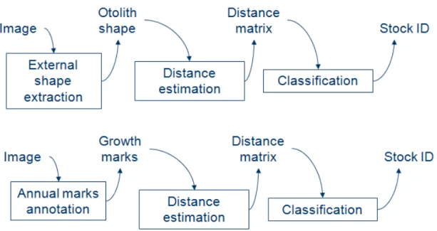
2.2. Shape-based stock identification 115 The shape-based classification process can be decomposed in three main 116 steps (Figure .2). First, the otolith contour is extracted as described in 117 next section (§ 2.2.1) using an automatic threshold. Three approaches to 118 extract reduced-dimension feature vectors from the contours were consid- 119 ered: Fourier Transform (FT), Principal Component Analysis (PCA) and 120 a technique issued from shape geodesics [Nasreddine et al., 2009]. The dis- 121 criminative power of each approach is evaluated using its own distance ma- 122 trix as input for a classifier. In other words, for a query input the feature 123 vector is considered as the distance matrix calculated between this indi- 124 vidual and the training individuals. Here, we investigate the performances 125 of two widely used classifiers: (1) the K-Nearest Neighbors (KNN) classi- 126 fier with the “leave-one-out” heuristic and (2) the Support Vector Machine 127 (SVM) classifier [Vapnik, 1995] with two randomly-selected sub-samples, one 128 of them is used to build the SVM-model which is tested on the other. 129

2.2.1. Automatic contour extraction 131 The otolith image is acquired using two imaging modalities: by trans- 132 mitted light or by reflected light. These two modalities could give additional 133 information. To extract the otolith outline, a mixed image is built in order 134 to integrate information available in both modalities (Figure .3). This mixed 135

(9)

image is a mean between the transmitted light image and the negative of 136 the reflected light image. Image contours are detected as local maximum 137 of the image gradient, approximated using a Sobel filtering. The resulting 138 contours are filled by a morphological closing operation and filtered to re- 139 tain the largest connected component which corresponds to the edge of the 140 otolith. The advantage of mixing both image modalities is illustrated on 141 example given by figure .3. The mixed image gives more details about the 142

contour especially on the region of the excisura major. 143

The resulting contour is then sampled into 300 points which describe 145

adequately the otolith shape. 146

2.2.2. Fourier descriptors 147

Shape can be described using complex Fourier descriptors [Granlund, 148 1972] or using elliptic Fourier descriptors [Kuhl and Giardina, 1982]. For 149 otolith shape analyses, both techniques have been extensively used and 150 proved to be efficient [Duarte-Neto et al., 2008a; Kristoffersen and Magoulas, 151 2008; M´erigot et al., 2007; Stransky et al., 2008a] [Cardinale et al., 2004; 152 Galley et al., 2006; Robertson and Talman, 2002; Schulz-Mirbach et al., 153 2008; Smith, 1992; Torres et al., 2000]. In our previous work [Nasreddine 154 et al., 2009] we have showed that for red mullet otoliths, classification results 155 are still similar by using these two methods. Elliptic Fourier descriptors are 156 more appropriate than complex Fourier descriptors when otolith contours 157 are composed of series of ellipse arcs (as for Trachurus mediterraneus otoliths 158 for example). Hence, for striped red mullet otoliths we have chosen to use 159 the complex descriptors which can be implemented more efficiently. 160 With a view to achieving translation, rotation and scaling invariance, 161

(10)

the first descriptor is aborted and the selected descriptors are scaled with 162 respect to the first non zero coefficient resulting in the so-called normalized 163

Fourier descriptors. The distance between two shapes is computed as the 164 Euclidean distance between the associated vectors of the normalized Fourier 165

descriptors. 166

2.2.3. Principal Component Analysis (PCA) 167 Principal Component Analysis (PCA) was first introduced by Pearson in 168 [Pearson, 1901] as a mathematical tool that transforms data linearly corre- 169 lated to uncorrelated variables called principal components. PCA is exten- 170 sively used in fisheries research for otolith shape analyses, in particular for 171 otolith stock identification. Usually, PCA is applied on Fourier coefficients 172 in order to assess differences in otolith shape [Duarte-Neto et al., 2008b; 173 M´erigot et al., 2007; Schulz-Mirbach et al., 2008]. PCA can also be applied 174 on morphometric variables [Torres et al., 2000], on a binary low resolution 175 image of the contour [Bermejo and Monegal, 2007] or for standardizing the 176

otolith contour orientation [Piera et al., 2005]. 177

However, PCA is not invariant to affine transformations, it is applied for 178 pattern recognition when the coordinates of input vectors can be ordered. 179 In face recognition for example, eyes and lips centers are manually selected, 180 then the images are rotated, in order to make the line connecting eye centers 181 horizontal, and resized to make the distances between the centers of the 182 eyes equal. The PCA is carried out on data vectors formed by cropped part 183 of images. In the case of calcified structures, it is not always obvious to 184 order the data vector coordinates on the basis of clearly defined landmarks. 185 A normalization procedure should then be applied to the raw contours to 186 be invariant with respect to translation, rotation and scaling, so that the 187

(11)

normalized shape is the result of the fish history, independently of acquisition 188

settings. 189

The translation invariance is obtained simply by subtracting the coordi- 190 nates of the mass center to the coordinates of all points. Scale invariance is 191 also simply obtained by dividing each point of the contour in polar coordi- 192 nates by the mean radius. For rotation normalization, a first solution could 193 be to align shapes according to the main axis. This axis can be defined by 194 the two farthest points of the shape or by minimizing the covariance using a 195 PCA like in [Piera et al., 2005]. However, on striped red mullet otolith, the 196 main axis does not correspond to a meaningful biological feature. Instead, 197 we propose to normalize shapes according to the center of excisura major. 198 The corresponding point of the excisura major can be detected automat- 199 ically after subtraction of the original otolith shape from the corresponding 200 filled shape. Then, each shape is aligned according to the axis that passes 201 through this point and the mass center of the otolith contour (Figure .4). 202

After contours normalization, PCA is applied on a matrix where each 204 of the rows represents a different contour and the columns represent the 205 information about the contours: the Cartesian normalized coordinates and 206 the local curvature are all put together in a row, one after the other. 207 To compute a distance between all contours in a given dataset, we pro- 208 ceed with a “leave-one-out” heuristics. One after another, each contour Ci 209 of the dataset is left out and PCA is computed on the remaining contours. 210 Then contour Ci is projected into the eigenspace generated by the eigenvec- 211 tors. Finally the distances between the projected contour and each of the 212 other projected contours of the dataset are computed as Euclidean distances 213

(12)

2.2.4. The geodesics approach 215 A potential drawback of Fourier and PCA approaches comes from the 216 implicit global (spatial) characterization of the shape. Each descriptor holds 217 information about all points of the shape as it is calculated using all points. 218 Therefore, local (spatial) discriminant shape signatures, such as shape dis- 219 continuities or landmarks, may not be well exploited by such a global char- 220 acterization [Parisi-Baradad et al., 2005]. In contrast, a Geodesic approach 221 was recently proposed [Nasreddine et al., 2009] to take advantage of lo- 222 cal shape features while ensuring invariance to geometric transformations 223 (e.g. translation, rotation and scaling). In this approach, we have defined 224 distance between shapes as a deformation cost stated as a matching issue, 225 i.e. determining the optimal matching between two otolith contours with 226

respect to a similarity measure. 227

The distance d(Γ1,Γ2) between two shapes Γ1 and Γ2 is stated as the 228 minimum, over all mapping functions Ψ, of the similarity measure, ED(Γ1, φ(Γ2229)) between the reference shape Γ1 and the mapped shape φ(Γ2). 230

d(Γ1,Γ2) = min

φ∈Ψ ED(Γ1, φ(Γ2)) (1)

As the important biological information is considered in the shape of 231 contour and not in its size, the shapes are parameterized in function of the 232 normalized curvilinear abscissa s which has a value between 0 and 1 inde- 233 pendently of the original contour length. A robust criterion is introduced in 234 order to improve the robustness of the proposed distance to outliers coming 235 from biological interindividual variabilities. The principle is supported by 236 the use of a function that adjusts weight ω in order to penalize the data 237

(13)

Given two shapes locally characterized by the angle θ(s) between the 239 tangent to the curve and the horizontal axis, the distance between two con- 240

tours is defined by: 241

d(θ1(s), θ2(s)) = 2 inf φ arccos Z s p φs(s) cosω(r(s))r(s) 2 ds (2)

where φs = dφ_ds and r(s) = θ1(s) − θ2(φ(s)). The term pφs(s) allows to 242 avoid torsion and stretching along the curve. The weight function ω is 243 issued from the robust estimator of Leclerc [Black and Rangarajan, 1996]; 244 ω(r(s)) = _σ22exp(

−r2_(s)

σ2 ) where σ is the standard deviation of data errors 245

r(s). 246

Formally, the numerical computation of d(Γ1,Γ2) is solved by using a 247 dynamic programming technique (refer to [Nasreddine et al., 2009] for more 248

details). 249

2.3. Growth marks based stock identification 250 The growth-based classification process consists of three main steps (Fig- 251 ure .2). First, an expert manually points out the growth marks on the 252 otolith image (Figure .5). This step can be done using TNPC software 253 (www.tnpc.fr) in parallel with the image acquisition step; it is not a contra- 254 diction with the automatic process of classification. Then distance between 255 the growth laws of two otoliths is computed using the Euclidean distances 256 between growth vectors. In case of two different aged otoliths, distance is 257 computed using only the growth marks available on both otoliths. For ex- 258 ample, in figure .5 this distance is computed using the three growth marks 259

on each otolith. 260

Given two growth vectors G1 = {G1j}j=1···N1 and G2 = {G2j}j=1···N2, 261 the growth distance is considered as the Euclidean distance: 262

(14)

dGrowth= v u u t Ng X j=1 (G2j− G1j)2 (3)

where Ng = min{N1, N2} is the number of growth marks available in both 263

vectors. 264

Finally, all distances between otoliths are computed leading to a distance 265 matrix used as input for an SVM classifier. The feature vector is consid- 266 ered as the distance calculated between the query input and all training 267

individuals. 268

3. Results 270

Here performances are evaluated in terms of correct classification rates. 271 We have started experiments with the hypothesis that the six stocks (NS, 272 EEC, WEC, CS, NBB and SBB) are considered as individual separated 273

stocks with specific characteristics of shapes. 274

Compared to KNN, SVM classifier performs slightly better in terms of 275 correct classification rate (from 30% to 32.7% on dataset (1)) but at the 276 cost of increasing dramatically the standard deviation of the performances 277 between classes (from 10.9 to 15.2 on dataset (1)). Thus, as KNN clas- 278 sifier results in stable performances across the classes, it has been chosen 279 for shape-based classification. In contrast, applying KNN for growth-based 280 stock identification gives a correct classification rate of 25.5% whereas SVM 281 gives higher correct classification rate (35.4%) for the same dataset (dataset 282 (1)). Hence, SVM has been chosen for growth-based classification. 283 The correct classification rates remain high with respect to the random 284 classification but these rates show that the hypothesis of separated stocks 285

(15)

should be aborted. The six stocks are then grouped into three stocks lead- 286 ing to a correct classification rate of 67%. Grouped stocks have in the first 287 hypothesis close shape characteristics and could not be really distinguished 288 easily. Classification errors could be due to genetic factors, migration among 289 others. A rate of 100% could then not be reached with the presence of all 290 these factors on the otolith shape. In comparisons to other stock identi- 291 fication methods, otolith shape is a promising approach but interpreting 292 patterns of variance can be difficult [Cadrin et al., 2005]. 293 In the following, geographical zones are ordered in the tables according 294 to their positions (from north (NS) to south (SBB)); thus neighbor classes 295

are also neighbor geographical zones. 296

3.1. Dataset (1) 297

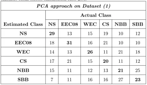
Results on dataset (1) are given in tables .1-.3. Geodesic approach 298 reaches 30% of correct classification (Table .3) while this rate is 19.7% for 299 Fourier approach (Table .1) and 25% for PCA (Table .2). These scores are 300 better than a random classification that would theoretically reach 16.7% (for 301

six classes). 302

{Table .1 goes here } 303

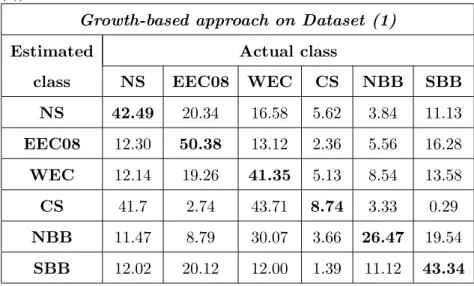
In table .4, classification results are given when the growth information 306 is used for stock identification. The mean correct classification obtained by 307

SVM reaches 35.4%. 308

As in [Nasreddine et al., 2009], we have tested stock identification with 310 both growth and shape information in order to improve classification per- 311

(16)

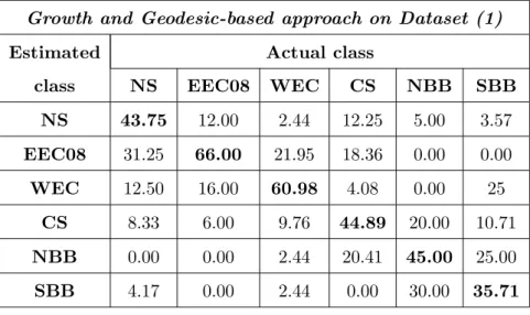
formances. The mean correct classification rate is then increased to reach 312

49.4% (Table .5). 313

3.2. Dataset (2) 315

On dataset (2), Fourier approach reaches 16.4% of mean correct clas- 316 sification (Table .6), PCA approach reaches 19% of correct classification 317 (Table .7) while Geodesic approach reaches 24.9% (Table .8). These scores 318 are also better than a random classification that would theoretically reach 319

14.3% (for seven classes). 320

3.3. Datasets (3) and (4) 324

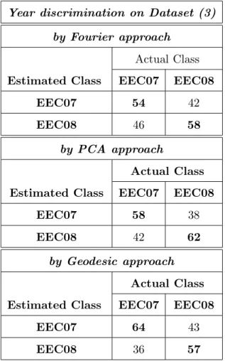
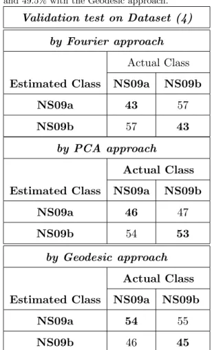
Regarding the year discrimination issue on dataset (3), the mean classi- 325 fication rate of the Fourier approach (56%, Table .9) is too close to the the- 326 oretical mean classification rate of a random classifier (50% for two classes). 327 Thus the classical Fourier approach fails on this specific year discrimination 328 issue. The mean classification rate on the random dataset (4) (43%, Ta- 329 ble .10) is lower but quite close to the theoretical mean classification rate of 330 a random classifier (50% for two classes), it shows that with this approach, 331 two arbitrary sets of the same stock and same year have no significant shape 332

differences. 333

Regarding PCA and Geodesic approaches, the mean classification rate 334 on dataset (3) (60%, Table .9) is higher than the mean classification rate 335 on the random dataset (4) (49.5%, Table .10). This shows that the otolith 336

(17)

morphology varies over two consecutive years and that this difference in 337 shape is higher than between two arbitrary groups of the same year and 338

same stock. 339

4. Discussion 342

4.1. Comparison of the three shape-based approaches 343 Performances of the three shape-based approaches are compared in ta- 344 ble .11. On both dataset (1) and dataset (2), the Geodesic approach exhibits 345 highest performances followed by PCA approach and Fourier approach last. 346 Regarding the stock discrimination issue on dataset (1) (Tables .1, .2 347 and .3), the three methods show that the population of striped red mullet 348

can be geographically divided in three zones: 349

• The Bay of Biscay (NBB+SBB) 350

• A mixing zone composed of the Celtic Sea and the Western English 351

Channel (CS+WEC) 352

• A northern zone composed of the Eastern English Channel and the 353

North Sea (EEC+NS) 354

To further the “three zones” hypothesis, we have tested the classification 355 when the otoliths were grouped in three classes corresponding to the three 356 zones. The results of this classification using the geodesic approach is shown 357 in table .12 below. It clearly validates the hypothesis as the obtained mean 358 correct classification rate reaches 54.3% and the error scores are higher be- 359 tween two neighbors zones than between two unconnected zones. Finally, 360

(18)

this rate raises to 67.31% when the SVM classifier is used with geodesic 361 distances coupled with the growth information (Table .13). 362 Regarding the year discrimination issue, classical Fourier approach fails 363 while PCA approach shows a small difference in shape and Geodesic ap- 364 proach exhibits the highest difference (Table .11). Thus Geodesic approach 365

seems the most appropriate method for this task. 366

4.2. Relevance of the shape and growth information 370 In this study three different approaches have been compared for shape- 371 based stock identification, two state-of-the-art methods (Fourier and PCA) 372 that have been extensively used in marine research on different species, and 373 a recent method (Geodesic) that proved to give very good performances 374 on different shapes [Nasreddine et al., 2010] and in particular on otolith 375 shapes [Nasreddine et al., 2009]. Although these three methods result in 376 high correct classification rates on several problems, they give quite low 377 correct classification rate for the particular cases tested in this study. It 378 tends to prove that otolith shape is not relevant for the particular case of 379 striped red mullet if we consider the six stocks separately. The growth- 380 based stock identification results are not so far from the shape-based stock 381 identification results. This study shows that both information are influenced 382 by different living conditions and different environments and can serve as 383 stock identifier. This identification is not very high as otolith shape is highly 384 due to the genetics. This result tends to prove that the genetic information 385 is quite homogeneously spread across all geographical zones in the north 386

(19)

west European seas. 387 This study has proven that by coupling both information (shape and 388 growth patterns), stock discrimination becomes more efficient. These two 389 information are independent and multivariate analysis, including them with 390 other independent information (chemical concentrations, . . . ), should be 391

investigated for stock identification. 392

The observations above lead to two hypothesis on the striped red mullet: 393

• some adults move from one zone to another, 394

• some larvae or juveniles perform migration during growth. 395

Acknowledgement 396

The authors want to thank the European commission for providing the 397 financial support of this work through the NESPMAN project, all scientists 398 and crew on board the RV “Thalassa” and the RV “Gwen Drez” for their 399

help with sample collection. 400

Apostolidis, A., Moutou, K., Stamatis, C., Mamuris, Z., 2009. Genetic struc- 401 ture of three marine fishes from the gulf of pagasitikos (greece) based on 402 allozymes, RAPD, and mtDNA RFLP markers. Biologia 64 (5), 1005– 403

1010. 404

Begg, G., Brown, R., 2000. Stock identification of haddock melanogrammus 405 aeglefinus on georges bank based on otolith shape analysis. Transactions 406

of the American Fisheries Society 129, 935–945. 407

Bermejo, S., Monegal, B., 2007. Fish age analysis and classification with 408 kernel methods. Pattern Recognition Letters 28 (10), 1164–1171. 409

(20)

Black, M., Rangarajan, A., 1 1996. On the unification of line processes, 410 outlier rejection, and robust statistics with applications in early vision. 411 International Journal of Computer Vision 19 (5), 57–92. 412 Burke, N., Brophy, D., King, P., 2008. Otolith shape analysis: its application 413 for discriminating between stocks of irish sea and celtic sea herring (clupea 414 harengus) in the irish sea. ICES Journal of Marine Science 65. 415 Cadrin, S., Friedland, K., Waldman, J., 2005. Stock identification methods: 416 Applications in Fishery science. Elsevier Academic press. 417 Campana, S., Casselman, J., 1993. Stock discrimination using otolith shape 418 analysis. Canadian Journal of Fisheries and Aquatic Sciences 50, 1062– 419

1083. 420

Cardinale, M., Doering-Arjes, P., Kastowsky, M., Mosegaard, H., 2004. Ef- 421 fects of sex, stock, and environment on the shape of known-age atlantic 422 cod (gadus morhua) otoliths. Canadian Journal of Fisheries and Aquatic 423

Sciences 61 (2), 158–167. 424

Carpentier, A., Martin, C., Vaz, S., 2009. Channel habitat atlas for ma- 425 rine resource management (charm phase ii). INTERREG 3a Programme, 426

IFREMER, Boulogne-sur-mer 65. 427

Desbrosses, P., 1933. Contribution `a la biologie du rouget-barbet en atlan- 428 tique nord. Revue des Travaux de l’Institut des Pˆeches Maritimes 6 (3), 429

249–270. 430

Desbrosses, P., 1935. Contribution `a la connaissance de la biologie du rouget 431 barbet en atlantique nord (iii) mullus barbatus (rond) surmuletus fage 432

(21)

mode septentrional fage. Revue des Travaux de l’Institut des Pˆeches Mar- 433

itimes 8 (4), 351–376. 434

Duarte-Neto, P., Lessa, R., Stosic, B., Morize, E., 2008a. The use of sagittal 435 otoliths in discriminating stocks of common dolphinfish (coryphaena hip- 436 purus) off northeastern brazil using multishape descriptors. ICES Journal 437

of Marine Science 65 (7), 1144–1152. 438

Duarte-Neto, P., Lessa, R., Stosic, B., Morize, E., 2008b. The use of sagittal 439 otoliths in discriminating stocks of common dolphinfish (coryphaena hip- 440 purus) off northeastern brazil using multishape descriptors. ICES Journal 441

of Marine Science 65, 1144–1152. 442

Galarza, J., Turner, G., Macpherson, E., Rico, C., 2009. Patterns of ge- 443 netic differentiation between two co-occurring demersal species: the red 444 mullet (mullus barbatus) and the striped red mullet (mullus surmuletus). 445 Canadian Journal of Fisheries and Aquatic Sciences 66 (9), 1478–1490. 446 Galley, E. A., Wright, P. J., Gibb, F. M., 2006. Combined methods of otolith 447 shape analysis improve identification of spawning areas of Atlantic cod. 448

ICES Journal of Marine Science 63 (9), 1710–1717. 449

Gordon, J., 1981. The fish populations of the west of scotland shelf. Part II, 450 Oceanography and Marine Biology. Annual Review 19, 405–441. 451 Granlund, G., 1972. Fourier preprocessing for hand print character recogni- 452

tion. IEEE Transanctions on Computers C-21, 195–201. 453

ICES, 2010. Report of the working group on assessment of new MoU species 454

(22)

Kristoffersen, J., Magoulas, A., 2008. Population structure of anchovy en- 456 graulis encrasicolus L. in the mediterranean sea inferred from multiple 457

methods. Fisheries research 91 (2-3), 187–195. 458

Kuhl, F., Giardina, C., 1982. Elliptic fourier features of a closed contour. 459

Computer Graphics and Image Processing 18, 236–258. 460

Mah´e, K., Destombes, A., Coppin, F., Koubbi, P., Vaz, S., Roy, D. L., Car- 461 pentier, A., 2005. Le rouget barbet de roche mullus surmuletus (L. 1758) 462 en manche orientale et mer du nord. Rapp. Contrat Ifremer/CRPMEM 463

Nord-Pas de Calais, 187p. 464

Mamuris, Z., Apostolidis, A., Theodorou, A., Triantaphyllidis, C., 1998a. 465 Application of random amplified polymorphic dna (rapd) markers to eval- 466 uate intraspecific genetic variation in red mullet (mullus barbatus). Marine 467

Biology 132, 171–178. 468

Mamuris, Z., Apostolidis, A., Triantaphyllidis, C., 1998b. Genetic protein 469 variation in red mullet (mullus barbatus) and striped red mullet (m. sur- 470 muletus) populations from the mediterranean sea. Marine Biology 130, 471

353–360. 472

Marchal, P., 2008. A comparative analysis of metiers and catch profiles for 473 some french demersal and pelagic fleets. ICES Journal of Marine Science 474

65, 674–686. 475

M´erigot, B., Letourneur, Y., Lecomte-Finiger, R., 2007. Characterization of 476 local populations of the common sole Solea solea (Pisces, Soleidae) in the 477 NW mediterranean through otolith morphometrics and shape analysis. 478

(23)

Nasreddine, K., Benzinou, A., Fablet, R., 2009. Shape geodesics for the clas- 480 sification of calcified structures: beyond fourier shape descriptors. Fish- 481

eries Research 98 (1-3), 8–15. 482

Nasreddine, K., Benzinou, A., Fablet, R., 2010. Variational shape matching 483 for shape classification and retrieval. Pattern Recognition Letters 31 (12), 484

1650–1657. 485

N’Da, K., Deniel, C., 1993. Sexual cycle and seasonal changes in the ovary 486 of the red mullet, mullus surmuletus, from the southern coast of brittany. 487

Journal of Fish Biology 43 (2), 229–244. 488

Parisi-Baradad, V., Lombarte, A., Garcia-Ladona, E., Cabestany, J., Piera, 489 J., Chic, O., 2005. Otolith shape contour analysis using affine transfor- 490 mation invariant wavelet transforms and curvature scale space represen- 491

tation. Marine and Freshwater Research 56, 795–804. 492

Pearson, K., 1901. On lines and planes of closest fit to systems of points in 493

space. Philosophical Magazine 2 (6), 559–572. 494

Piera, J., Parisi-Baradad, V., Garcia-Ladona, E., Lombarte, A., Recasens, 495 L., Cabestany, J., 2005. Otolith shape feature extraction oriented to au- 496 tomatic classification with open distributed data. Marine and freshwater 497

research 56 (5), 805–814. 498

Poulard, J., Blanchard, F., 2005. The impact of climate change on the fish 499 community structure of the eastern continental shelf of the bay of biscay. 500

ICES Journal of Marine Science 62, 1436–1443. 501

(24)

tion structure of marine fish: mismatch between biological and fisheries 503

management units. Fish and Fisheries 10, 361–395. 504

Robertson, S., Talman, S., 2002. Shape analysis and ageing of orange roughy 505 otoliths from the south tasman rise. Tech. rep., Final Report to the 506 Australian Fisheries Management Authority. Marine and Freshwater Re- 507

sources Institute. 508

Schulz-Mirbach, T., Stransky, C., Schlickeisen, J., Reichenbacher, B., 2008. 509 Differences in otolith morphologies between surface- and cave-dwelling 510 populations of Poecilia mexicana (teleostei, poeciliidae) reflect adapta- 511 tions to life in an extreme habitat. Evolutionary Ecology Research 10 (4), 512

537–558. 513

Smith, M. K., 1992. Regional differences in otolith morphology of the deep 514 slope red snapper etelis carbunculus. Canadian Journal of Fisheries and 515

Aquatic Sciences 49 (4), 795–804. 516

Smith, P., Francis, R., McVeagh, M., 1991. Loss of genetic diversity due to 517

fishing pressure. Fisheries Research 10, 309–316. 518

Stransky, C., 2005. Geographic variation of golden redfish (sebastes marinus) 519 and deep-sea redfish (s. mentella) in the north atlantic based on otolith 520 shape analysis. ICES Journal of Marine Science 62, 1691–1698. 521 Stransky, C., Baumann, H., Fevolden, S.-E., Harbitz, A., Hie, H., Nedreaas, 522 K. H., Salberg, A.-B., Skarstein, T. H., 2008a. Separation of norwegian 523 coastal cod and northeast arctic cod by outer otolith shape analysis. Fish- 524

(25)

Stransky, C., Murta, A., Schlickeisen, J., Zimmermann, C., 2008b. Otolith 526 shape analysis as a tool for stock separation of horse mackerel (trachurus 527 trachurus) in the northeast atlantic and mediterranean. Fisheries Research 528

89, 159–166. 529

Torres, G. J., Lombarte, A., Morales-Nin, B., 2000. Sagittal otolith size 530 and shape variability to identify geographical intraspecific differences in 531 three species of the genus merluccius. Journal of the Marine Biological 532

Association of the UK 80 (2), 333–342. 533

Vapnik, V., 1995. The nature of statistical learning theory. Springer-Verlag, 534

New York, USA. 535

Wheeler, A., 1978. Key to the fishes of northern europe. Frederick Warne & 536

(26)

(27)

Figure .2: Shape-based and growth-based classification general schemes.

Figure .3: Contour extraction using transmitted light image (left), reflected light image (middle) and resulting mixed image (right). Note that the contour extracted using the mixed image is more efficient.

(28)

Figure .4: Contour extraction and normalization. Left: contour before normalization, right: contour after rotation normalization. In this figure we show the main axis passing through the mass center and the excisura major center.

(a) (b)

Figure .5: Illustration of growth distance calculation. (a): Annual growth marks manually positioned by expert. (b): Example of distance computation between growth laws of two otoliths.

(29)

Table .1: Confusion matrix (in %) for the Fourier approach on dataset (1) achieved by KNN classifier. Mean correct classification rate: 19.7%.

Fourier approach on Dataset (1) Actual Class

Estimated Class NS EEC08 WEC CS NBB SBB

NS 18 20 11 18 18 12 EEC08 21 28 25 17 6 14 WEC 8 19 12 16 7 14 CS 21 12 18 13 11 14 NBB 16 9 14 16 23 22 SBB 16 12 20 20 35 24

Table .2: Confusion matrix (in %) for the PCA approach on dataset (1) achieved by KNN classifier. Mean correct classification rate: 25%.

PCA approach on Dataset (1) Actual Class

(30)

Table .3: Confusion matrix (in %) for the Geodesic approach on dataset (1) achieved by KNN classifier. Mean correct classification rate: 30%.

Geodesic approach on Dataset (1) Actual Class

Table .4: Confusion matrix resulting from an SVM classifier on growth distances (dataset (1)). Mean correct classification rate: 35.4 %.

Growth-based approach on Dataset (1)

Estimated Actual class

class NS EEC08 WEC CS NBB SBB

NS 42.49 20.34 16.58 5.62 3.84 11.13 EEC08 12.30 50.38 13.12 2.36 5.56 16.28 WEC 12.14 19.26 41.35 5.13 8.54 13.58 CS 41.7 2.74 43.71 8.74 3.33 0.29 NBB 11.47 8.79 30.07 3.66 26.47 19.54 SBB 12.02 20.12 12.00 1.39 11.12 43.34

(31)

Table .5: Confusion matrix resulting from an SVM classifier on geodesic distances coupled with growth distances (dataset (1)). Mean correct classification rate: 49.4 %.

Growth and Geodesic-based approach on Dataset (1)

Estimated Actual class

class NS EEC08 WEC CS NBB SBB

NS 43.75 12.00 2.44 12.25 5.00 3.57 EEC08 31.25 66.00 21.95 18.36 0.00 0.00 WEC 12.50 16.00 60.98 4.08 0.00 25 CS 8.33 6.00 9.76 44.89 20.00 10.71 NBB 0.00 0.00 2.44 20.41 45.00 25.00 SBB 4.17 0.00 2.44 0.00 30.00 35.71

Table .6: Confusion matrix (in %) for the Fourier approach on dataset (2) achieved by KNN classifier. Mean correct classification rate: 16.4%.

Fourier approach on Dataset (2) Actual Class

Estimated Class NS EEC07 EEC08 WEC CS NBB SBB

NS 15 10 22 7 18 13 11 EEC07 15 19 12 23 14 11 11 EEC08 17 16 24 18 17 7 11 WEC 6 17 14 7 14 5 11 CS 20 14 8 17 7 12 11 NBB 16 14 8 12 15 20 22 SBB 11 10 12 16 15 32 23

(32)

Table .7: Confusion matrix (in %) for the PCA approach on dataset (2) achieved by KNN classifier. Mean correct classification rate: 19%.

PCA approach on Dataset (2) Actual Class

Table .8: Confusion matrix (in %) for the Geodesic approach on dataset (2) achieved by KNN classifier. Mean correct classification rate: 24.9%.

Geodesic approach on Dataset (2) Actual Class

(33)

Table .9: Confusion matrix (in %) on dataset (3) achieved by KNN classifier. Mean correct classification rate: 56% with the Fourier approach, 60% by the PCA approach and 60.5% with the Geodesic approach.

Year discrimination on Dataset (3) by Fourier approach

Actual Class

Estimated Class EEC07 EEC08

EEC07 54 42

EEC08 46 58

by PCA approach

Actual Class

EEC07 58 38

EEC08 42 62

by Geodesic approach Actual Class

EEC07 64 43

(34)

Table .10: Confusion matrix (in %) on dataset (4) achieved by KNN classifier. Mean correct classification rate: 43% with the Fourier approach, 49.5% by the PCA approach and 49.5% with the Geodesic approach.

Validation test on Dataset (4) by Fourier approach

Actual Class

Estimated Class NS09a NS09b

NS09a 43 57

NS09b 57 43

by PCA approach

Actual Class

NS09a 46 47

NS09b 54 53

by Geodesic approach Actual Class

NS09a 54 55

(35)

Table .11: Comparison of the mean correct classification rate (in %) obtained by the three approaches on datasets (1), (2) and (3) achieved by KNN classifier.

dataset (1) Dataset (2) Dataset (3)

Fourier 19.7 16.4 56

PCA 25 19 60

Geodesic 30 24.9 60.5

Table .12: Classification results on dataset (1) with the Geodesic approach when the otoliths were grouped in three classes according to their geographical zones. Mean correct classification rate: 54.3% (KNN classifier).

Geodesic approach on Dataset (1) with otoliths grouped by zones

Actual Class

Estimated Class Northern zone Mixing zone Bay of Biscay

Northern zone 53.5 29.5 13

Mixing zone 28.5 44.5 22

(36)

Table .13: Classification results (in %) on dataset (1) with the Growth and Geodesic-based approach when the otoliths were grouped in three classes according to their geographical zones. Mean correct classification rate: 67.31% (SVM classifier).

Growth and Geodesic-based approach on Dataset (1) with otoliths grouped by zones Actual Class

Estimated Class Northern zone Mixing zone Bay of Biscay

Northern zone 74.30 26.76 8.61

Mixing zone 22.31 58.25 22.00