Guidance document on sampling, analysis and counting standards for phytoplankton in lakes: WISER Deliverable D3.1-4

(1)

HAL Id: hal-02597293

https://hal.inrae.fr/hal-02597293

Submitted on 15 May 2020

HAL is a multi-disciplinary open access archive for the deposit and dissemination of sci-entific research documents, whether they are pub-lished or not. The documents may come from teaching and research institutions in France or abroad, or from public or private research centers.

L’archive ouverte pluridisciplinaire HAL, est destinée au dépôt et à la diffusion de documents scientifiques de niveau recherche, publiés ou non, émanant des établissements d’enseignement et de recherche français ou étrangers, des laboratoires publics ou privés.

standards for phytoplankton in lakes: WISER

Deliverable D3.1-4

U. Mischke, S. Thackeray, M. Dunbar, C. Mac Donald, L. Carvalho, C. de

Hoyos, M. Järvinen, Christophe Laplace-Treyture, G. Morabito, B. Skjelbred,

et al.

To cite this version:

U. Mischke, S. Thackeray, M. Dunbar, C. Mac Donald, L. Carvalho, et al.. Guidance document on sampling, analysis and counting standards for phytoplankton in lakes: WISER Deliverable D3.1-4. [Research Report] irstea. 2012, pp.51. �hal-02597293�

(2)

1

Collaborative Project (large-scale integrating project) Grant Agreement 226273

Theme 6: Environment (including Climate Change) Duration: March 1st_{, 2009 – February 29}th_{, 2012}

Deliverable D3.1-4:

Guidance document on sampling,

analysis and counting standards for phytoplankton in

lakes

Lead contractor: (IGB)

Contributors: Ute Mischke, Stephen Thackeray, Michael Dunbar, Claire McDonald, Laurence Carvalho, Caridad de Hoyos, Marko Jarvinen, Christophe Laplace-Treyture, Giuseppe Morabito, Birger Skjelbred, Anne Lyche Solheim, Bill Brierley and Bernard Dudley

Due date of deliverable: Month 33 (November 2011) Actual submission date: Month 36 (February 2012)

Project co-funded by the European Commission within the Seventh Framework Programme (2007-2013)

Dissemination Level

PU Public X

PP Restricted to other programme participants (including the Commission Services) RE Restricted to a group specified by the consortium (including the Commission

Services)

CO Confidential, only for members of the consortium (including the Commission Services)

(3)

2

Content

Content ... 2

Introduction ... 3

Recommendations for sampling, analysis and counting ... 3

Sampling method ... 4

Frequency of sampling ... 7

Analysis and counting standards ... 11

Operational European taxa list phytoplankton – WISER code list ... 11

Activities to harmonize determination of biovolume ... 12

References ... 13

Annex 1: WISER Guidance on phytoplankton counting ... 15

(4)

3

Introduction

Sampling, analysis and counting of phytoplankton has been undertaken in European lakes for more than 100 years (Apstein 1892, Lauterborn 1896, Lemmermann 1903, Woloszynska 1912, Nygaard 1949). Since this early period of pioneers, there has been progress in the methods used to sample, fix, store and analyse phytoplankton. The aim of the deliverable D3.1-4 is to select, harmonize and recommend the most optimal method as a basis for lake assessment. We do not report and review the huge number of European national methods or other published manuals for phytoplankton sampling and analysis that are available.

An agreement on a proper sampling procedure is not trivial for lake phytoplankton. In the early 20th century, sampling was carried out using plankton nets. An unconcentrated sample without any pre-screening is required for quantitative phytoplankton analysis, for which various water samplers were developed. Sampling of distinct water depths or an integral sample of the euphotic zone affects the choice of the sampler and sampling procedure.

The widely accepted method to quantify algal numbers together with species determination was developed by Utermöhl (1958), who proposed the counting technique using sediment chambers and inverse microscopy. This is the basis for the recently agreed CEN standard “Water quality - Guidance standard on the enumeration of phytoplankton using inverted microscopy (Utermöhl technique)” (CEN 15204, 2006). This CEN standard does not cover the sampling procedure or the calculation of biovolumes for phytoplankton species, although Rott (1981), Hillebrand et al (1999) and Pohlmann & Friedrich (2001) have contributed advice on how to calculate taxa biovolumes effectively. Willén (1976) suggested a simplified counting method, when counting 60 individuals of each species. For the Scandinavian region an agreed phytoplankton sampling and counting manual was compiled, which has been in use for about 20 years (Olrik et al. 1998, Blomqvist & Herlitz 1998).

It is very unfortunate that no European guidance on sampling of phytoplankton in lakes was agreed before the phytoplankton assessment methods for the EU-WFD were developed and intercalibrated by Member States. In 2008 an initiative by the European Commission (Mandate M424) for two draft CEN standards on sampling in freshwaters and on calculation of phytoplankton biovolume was unfortunately delayed by administrative difficulties. Recently a grant agreement was signed between the Commission and DIN (German Institute for Standardization) in January 2012 to develop these standards. We believe this WISER guidance document can usefully contribute to these up-coming standards.

Recommendations for sampling, analysis and counting

This guidance report is not a systematic review of all possible and applied strategies, but refers to experiences from both within and outside of the WISER project. A common sampling strategy for phytoplankton in lakes is proposed here, based on agreement on a

(5)

4

common sampling method amongst national phytoplankton experts for adoption in the WISER field campaign. Recommendations on sampling locations and frequency are based on new analysis carried out in WISER on spatial and temporal sources of uncertainty in metric scores (Thackeray et al. 2011; 2012 – See Annex 2). A survey of sampling methods and frequencies for phytoplankton in lakes reported by European countries for EU-WFD methods (Birk et al. 2010 and milestone 6 reports) was also used in developing this recommended guidance (Table 1).

Table 1: Sampling method and frequency for phytoplankton in lakes reported by European countries for EU-WFD methods (for details see Birk et al. 2010 and milestone 6 reports)

sampling integral

vertical depth integral if lake is thermal stratified

frequency per year for PP taxa . (at least) frequency chlorophyll a . (at least) N years must be included for assessment Yes (N = 17) euphotic (N = 14) > 4 samples

(N = 6) > 5 samples (N = 7) 3 years (N = 4) tube 0-2m -14) (N = 2) epilimnion (N = 3) 4 samples (N = 5) 4 samples (N = 6) No (4) subsurface depth ( N = 4) 3 samples (N = 4) 3 samples (N = 4) shoreline/outlet (N = 1) 2 samples (N = 4) 2 samples (N = 4) 1 samples (N = 3) 1 samples (N = 1)

Sampling method

How representative is one sample per lake?

The effects of sample location and replicate sampling within a lake were examined in the WISER field exercise (Thackeray et al. 2011; WISER Deliverable 3.1-3). This work revealed that variability in metric scores is largely due to variability between lakes and that this is significantly related to differences in eutrophication pressure (total phosphorus concentrations). Differences in locations around a lake, sample replicates or analytical variability only account for a small proportion of the variability in metric scores (Table 2). These results were especially true for the three types of phytoplankton metric being used by many Member States: chlorophyll a concentration, PTI and cyanobacteria abundance, for which >85% of the variability in metric scores was attributed between lakes. Although these metrics were very robust to differences in the location of sampling points within a lake, it has to be stressed that the WISER field campaign only compared three different open water locations: the deep point, the mean depth point and an intermediate depth. It did not examine sampling from the edge, the outflow or separated bays and so cannot be used to approve or disapprove of any method based on these locations. It did, however, highlight that only a single open water location needs to be sampled and replicate sampling will have little benefit on uncertainty in status assessments.

(6)

5

Table 2. Proportions of metric variance for different sources of variability for six candidate phytoplankton metrics. Total between = Country + Waterbody, Total within = Station + Sample + Analyst + Error(sub-sample). Table taken from Thackeray et al., 2011)

Metric Country Waterbody Station Sample Analyst Error (sub-sample) Total within Total between Chl 0.00 0.96 0.01 0.01 - 0.02 0.04 0.96 PTI 0.00 0.88 <0.01 0.00 0.04 0.07 0.12 0.88 SPI 0.00 0.65 0.03 0.00 0.19 0.13 0.35 0.65 MFGI 0.00 0.86 0.02 <0.01 0.05 0.08 0.14 0.86 FTI 0.00 0.81 0.02 0.00 0.09 0.08 0.19 0.81 Evenness 0.00 0.69 0.04 0.00 0.17 0.10 0.31 0.69 Log total cyanobacteria 0.09 0.86 0.01 0.00 0.02 0.03 0.06 0.94

These results were true for the 31 WISER lakes in the field exercise, but it should be stated that it is not always true. For example, it has been shown that in small, well sheltered lakes small-scale horizontal patchiness of the phytoplankton can result in differences in assessment results (Borics et al., 2011). There are also some more predictable exceptions, where spatial heterogeneity can be expected to be greater, where more than 1 sampling location should be considered. This includes large lakes (e.g. surface area >10 km²) or lakes with clearly distinct separated bays. In these cases, several integrated samples could be taken and mixed before analysis. If external pressures are likely to impact differently in different basins of large, morphologically complex lakes, then these basins should be designated as distinct water bodies and assessed separately. Finally, with the development of satellite technology in the near future, high resolution, multi-spectra satellite imagery may enable improved spatial representation of the open-water of large lakes for parameters such as chlorophyll a and cyanobacteria biovolume (Hunter et al., 2010).

Vertical integrated samples from various water depths

Sampling distinct depths, such as 0.5 m depth, can be unrepresentative due to vertical heterogeneity in phytoplankton, which can form distinct layers in calm situations as a result of light over saturation, algal scums at the surface or deep layer maxima. In short, distinct depth samples do not represent the whole water column within which phytoplankton can grow. This is overcome in most European lakes and countries, by analysing phytoplankton from integrated depth samples, such as from the epilimnion or the euphotic zone. Each strategy has its advantages and disadvantages.

The euphotic zone (Zeu) is defined by the depth to which 1% of surface light penetrates or, more pragmatically, 2.5 times the water transparency measured by Secchi depth. In clear lakes the euphotic zone can be deeper than the epilimnion, surpassing the depth of the thermal summer stratification (Zepi), and deep chlorophyll a maxima may develop. In Central

(7)

6

Europe wind protected deep lakes can have anoxic hypolimnion even at mesotrophic status (example is Roofensee, DE with high status), which would be integrated into a sample from the euphotic zone; in such cases integrated sampling of the epilimnion is recommended. In very turbid lakes integrated sampling from the epilimnion may also be a better choice, because the euphotic zone may be much shallower than the epilimnion, when temporal micro-stratifications enable algal bloom layers above the steepest thermally stratified layer in calm weather conditions. Some countries decided to use epilimnetic sampling in cases where Zeu < Zepi (Table 1).

In most European countries WFD sampling is carried out at the deepest point of the lake and from the euphotic zone (see Table 1). This sampling strategy is underpinned by the investigations of Nõges et al. (2010) who showed that in thermally stratified lakes, 2.5 * Secchi depth proved a suitable criterion of the sampling depth and only in the case of surface scums, would sampling of a 3 * Secchi depth layer be recommended in order not to miss the deep chlorophyll maximum.

WISER recommendation on sampling methodology

In summary, to ensure maximum consistency across Europe, we recommend the following sampling strategy for phytoplankton biomass (including chlorophyll a), taxonomic composition and bloom metrics:

• To best represent the whole of the phytoplankton community, vertically integrated samples should be taken from the euphotic zone in thermally stratified lakes and reservoirs. (2.5 x Secchi depth). Integrated samples from the epilimnion may, however, be a better alternative when Zeu < Zepi

• To avoid contamination and edge effects, samples should be taken from the deepest point of a lake, or similar open-water location. When the lake is large or has a complex morphology, the sample from the deepest point could be mixed with other samples from additional open-water locations to represent the water body as a whole. For harmonization of methods across Europe, we strongly recommend Member States consider changing their sampling strategy if they undertake the following:

• If only one distinct depth (e.g.0.5m) is sampled when the lake is stratified, Member States should strongly consider changing to an integrated sample of the euphotic zone. • If sampling is only carried out at the lake edge or outlet, there is a strong risk of contamination with benthic algae and edge effects. Unless it can be shown that the outlet sample is representative of that particular lake, Member States should change to open-water sampling.

(8)

7

Frequency of sampling

The engagement and ambition to capture seasonal succession and variability greatly differs between European countries. Sampling frequencies vary from twice in the vegetation period to monthly sampling throughout the year (Table 1). These variations in sampling can contribute to differences between assessment results and may require different status class standards (e.g. some countries may set chlorophyll standards based on growing season means whilst other countries standards may be based on annual means). Additionally, different definitions of growing season can make it difficult to apply all methods consistently to all data. For example data from late summer only should not be applied to classification schemes which are based on taxonomic composition over the full growing season.

A strict and agreed definition for the growing season is not, however, possible across Europe. The duration and the onset of the ice-free period vary by longitude (Atlantic influence), latitude (Finland to Spain) and altitude. Despite this, it is evident that the period from July to August is a common period for phytoplankton sampling in European lakes (Fig. 1), and is a period in which many phytoplankton composition metrics can be applied.

Figure 1: Distribution of samples in months, which were analyzed for taxonomic composition to

assess European lakes taken from WISER 3.1 data base.N = Nordic region; M = Mediterranean region, EC = Eastern Central region; CB = Central Baltic region.

Figure 2 demonstrates the effect of various sampling frequencies on representing the “true” annual mean based on at least 26 samples per year (Carvalho et al. 2006). The probability of mis-classification is always at least 50% at the good/moderate boundary, but because the standard deviation is low when averaging 26 samples, the probability to mis-classify strongly decreases from the boundary value. In contrast, the mis-classification risk remains very high when only one sample per year of the 26 possible samples is used to represent the annual

0 500 1000 1500 2000 2500 3000 3500 4000

Jan Feb Mar Apr May Jun Jul Aug Sep Oct Nov Dec

N sam ple s with Ut er m öhl c oun ts N M EC CB

(9)

8

mean. Due to ease of measurement, chlorophyll a concentrations are often determined more frequently than phytoplankton composition. Figure 2 suggests that at least monthly sampling should be carried out at this shallow lake, and similar results were found for a deep lake. In countries with a low monthly sampling frequency the assessment can be made less uncertain by using data from 3 or more years of monitoring, thus increasing the number of samples used for assessment (Table 3). The statistical evidence for this is provided in Annex 2 (Thackerey et al 2012).

Figure 2: Effect of within-year sampling frequency on the probability of ecological status

mis-classification at the good/moderate boundary for chlorophyll a concentrations (redrawn from Carvalho et al. 2006).

Phytoplankton data collated in the WISER project from more than 3000 European lakes were used to carry out analyses to compare temporal and between-lake variation in phytoplankton metrics at the GIG scale (Annex 2: Thackeray et al. 2012). The three focal metrics were chlorophyll a concentration, PTI (Phillips et al. 2010) and total cyanobacterial biovolume (Carvalho et al in Mischke et al. 2010). Thackeray et al. (2012) produced results on the relative magnitude of temporal (inter-annual and monthly) and spatial (between-waterbody/country) metric variation. They used the estimated temporal variance components to describe changes in the degree of uncertainty in the observed value of each metric for a waterbody, when based upon collecting samples from different numbers of years, and/or months within years. As a result of this analysis, Table 3 summarises the minimum recommended sampling frequencies for the three metrics in three GIGs. Where possible, two alternative sampling frequencies have been recommended for a given metric to give Member

(10)

9

States more flexibility in their operational monitoring programmes, but retaining comparable confidence in classification.

Table 3. Minimum recommended sampling frequencies for three metrics in three GIGs

CB-‐GIG M-‐GIG N-‐GIG

Chlorophyll a 3 months for 4 years 3 months for 3 years or 3 months for 2 years 2 months for 3 years PTI or 1 month for 6 years 2 months for 4 years or 1 month for 6 years 3 months for 3 years or 1 month for 6 years 3 months for 3 years Cyanobacteria 1 month for 6 years 1 month for 6 years 1 month for 6 years

For example, for the chlorophyll a-metric, the sampling variance (and associated uncertainty) reduces markedly when increasing the number of months sampled from 1 per year to 3 per year and sampling in 2 or 3 years, instead of 1 (Fig. 3). The N-GIG analyses suggest that sampling variance is similar if sampling in 2 months in each of 3 years compared with 3 months in each of 2 years, but due to the higher level of temporal variability for chlorophyll a in CB-GIG, a greater degree of replication is needed to achieve this same reduction in sampling variance (a minimum of 3 months in each of 4 years).

Thackeray et al., (2012: Annex 2) do also highlight that the seasonality of different metrics is often affected by a number of factors, such as latitude, longitude, altitude and TP and that sampling strategies should ideally be adaptive based on these. For European consistency, WISER recommends that the sampling season should always include the July-August period. In Southern Europe June is a common sampling month and may be best for the third month, whilst in Northern Europe September may be more appropriate. Ideally, sampling should be representative of the whole phytoplankton seasonal succession (e.g., in Mediterranean Countries 1 sampling in the period April-May and 1 in October may also be considered). It should, however, be noted that the reported uncertainties for the PTI and cyanobacteria biovolume metrics in Annex 2 are based on Jul-Sep data and uncertainties may differ if a different seasonal window is used.

The analyses of temporal variation did also suggest that unexplained (residual) variation was quite high for some metric/GIG combinations. This was particularly true for the cyanobacterial biovolume metric in N-GIG and Med-GIG and the PTI in the CB-GIG and Med-GIG. The residual variance is the variance that cannot be explained by the factors we used in the statistical analysis (i.e. the temporal (month and year) and the spatial parameters (lake and country)). This residual variation could be due to shorter-term (within month) metric variation, but may also represent variability due to within-lake location or analyst

(11)

10

variability. The uncertainty analysis from the WISER field exercise (D3.1-3, Thackeray et al., 2011) indicated that analyst variability was generally the highest source of within-lake variability and can be minimised by standardising sampling and analysis methods and effective training between different counters (see “Analysis and counting standards” section and Annex 1 for recommendations). For the total cyanobacterial biovolume metric this residual variance may be very high because of the high number of zero values in N-GIG and Med-GIG for this metric resulting in a very large range between the low and high values of the metric.

Fig. 3. Changes in monthly and inter-annual scale temporal sampling variance for chlorophyll a, assuming monitoring schemes which differ in the number of years and months-per-year sampled. Analysis based upon the cross-GIG data set

(12)

11

Analysis and counting standards

In order to harmonize phytoplankton count data for the WISER field exercise, three phytoplankton workshops, including more than 30 phytoplankton experts, were held throughout Europe in 2009 to discuss counting strategies and standardise taxonomy and biovolume measurements:

• Nordic region at SYKE in Helsinki, September 10-11 organized by Marko Jarvinen • Central Baltic European region at IGB in Berlin, September 21-22 organized by Ute

Mischke

• Mediterranean region at CEDEX in Madrid, October 22-23 organized by Caridad de Hoyos

The final WISER counting method “Guidance: the quantitative analysis of phytoplankton” is provided in Annex 1 of this report. It was agreed following a survey of national methods and comments from all three workshops. This counting method may differ from some national methods for analysing WFD samples, but our survey showed that it compares closely to methods adopted by many countries. The WISER counting guidance was based on the inverted microscopy techniques described in Utermöhl (1958) and the CEN (2006) guidance standard for the routine analysis of phytoplankton. WISER added recommendations on counting effort and a counting strategy that included counts at:

1) low magnification (40x or 100x), a whole chamber count of large taxa, followed by; 2) 2 transect counts at an intermediate magnification (200x or 250x), to enumerate “intermediate-sized” taxa (>20 µm) that are too small for the low-magnification count but too rare to be reasonably counted using fields of view at high magnification, followed by;

3) a high magnification count (x400 or greater) using fields of view to pick up the small and more common taxa. Aim to count 50-100 fields of view (i.e. at least 400 taxa units assuming the recommended sample concentration).

All details are described in Annex 1.

Operational European taxa list phytoplankton – WISER code list

To harmonize the European phytoplankton data, a European taxa list was produced within the WISER project. This list was based on the former list established for the EU Rebecca project and was refined, prolonged and elongated by further information. Regional schools and traditions, competing systematic systems and increasing molecular knowledge lead to diverse names for the same morpho-types designated by different determination keys. So more than 5000 taxa were checked and merged to a final list of about 2300 taxa.

The phytoplankton list was used as the basis to produce a Taxa Entry Tool (TET) & Taxa Validation Tool (TVT) (see http://www.freshwaterecology.info/; Mischke et al. 2012).

(13)

12 The list offers for users and for data bases:

(1) Code numbers for all quantitatively relevant taxa of plankton

(2) Easy sorting for genus, order and class level within a common systematic classification system

(3) Taxonomically valid names (status year 2010) a) Offering a synonym list

b) Providing the author of first description and year of description (4) Highlighting marine and heterotrophic taxa.

What is still missing?

Expert network: Persons in charge for taxonomic groups in all eco-regions European or national centre for quality insurance

The European WISER list was created as an operational list to merge European data and to develop indicator systems. So the WISER phytoplankton list is not kept up to date with new valid names. These can be checked against other online taxonomic sources, such as the webpage http://www.algaebase.org/.

Activities to harmonize determination of biovolume

A draft of a CEN proposal for biovolume determination was prepared by Germany in 2008, to cover marine and freshwater analysis of phytoplankton. This draft (Water quality — Phytoplankton biovolume determination by microscopic measurement of cell dimensions) will be tested in an inter-laboratory comparison in the up-coming DIN project under the Mandate 424. The aim is to provide a complete list of genus names and, if deviating in shape, of species names connected to the most proper geometric shapes, indicating the cell dimensions to measure and the calculation equations. The HELCOM checklist of Baltic Sea Phytoplankton Species is a useful starting point listing the marine taxa with geometric shapes (Hillebrand et al, 1999, Olenina et al. 2006). Further pure freshwater taxa must be added to this list.

(14)

13

Table A.1 (continued) Example redrawn from draft CEN proposal

Geometric shape Illustration Equation

Sickle shaped cylinder (synonyms: Sickle shaped prism) V = 1/4 * π *h * (d1* d2 - d3* d4)

References

Apstein, C. (1892): Quantitative Plankton-Studien im Süßwasser. Biologisches Zentralblatt 12 (16/17): 484-512

Birk, S., Strackbein, J. & Hering, D. (2010): WISER methods database. Version: March 2011. Available at http://www.wiser.eu/results/method-database/.

Blomqvist P. & Herlitz E. (1998): Methods for quantitative assessment of phytoplankton in freshwaters. Part II: Literature and its use for determination of planktic volvocales, tetrasporales, chlorococcales, and ulotrichales and formulas for calculation of biovolume of the organisms 4861Rapport. ISBN: 91-620-4861-9, Naturvårdsverket, Stockholm, 68 pp.

Borics G,Abonyi, A., Krasznai E., Várbíró G., Grigorszky I., Szabó S., Deák Cs. & Tóthmérész B. (2011): Small-scale patchiness of the phytoplankton in a lentic oxbow. Journal of plankton research 33(6): 973-981.

Carvalho, L., Phillips, G., Maberly, S.C. & Clarke, R. (2006): Chlorophyll and Phosphorus Classifications for UK Lakes, SNIFFER, Edinburgh, Environment Agency, Project WFD38, Final report, 81 pp.

CEN EN 15204, 2006. Water quality – Guidance standard for the routine analysis of phytoplankton abundance and composition using inverted microscopy (Utermöhl technique)

Hillebrand, H., C.-D. Dürselen, D. Kirschtel, U. Pollingher, & T. Zohary (1999): Biovolume calculation for pelagic and bentic microalgae. Journal of Phycology 35: 403-424

Hunter, P.D., Tyler, A.N., Carvalho, L., Codd., G.A. and Maberly, S.C. 2010. Hyperspectral remote sensing of cyanobacterial pigments as indicators for cell populations and toxins in eutrophic lakes. Remote Sensing of Environment, 114: 2705-2718.

Lauterborn, R. (1896): Ueber das Vorkommen der Diatomeen-Gattungen Atheya und Rhizosolenia in den Altwassern des Oberrheins. Bericht der Deutschen Botanischen Gesellschaft 14: 11-15 Lemmermann, E. (1903): Brandenburgische Algen II. Das Phytoplankton des Müggelsees und einiger

benachbarter Gewässer. Zeitschrift für Fischerei Heft 2, Jahrg. 9: 73-123

Mischke U., Skjelbred B., Morabito, G., Ptacnik R., de Hoyos C., Negro A.I., Laplace C., Kusber W.-H., Bijkerk R., Phillips G., Solheim A.L., Borics, G. & Carvalho L. (2012): Phytoplankton Indicator Database according to the WISER project; www.freshwaterecology.info, version 5.0) Mischke, U., Carvalho, L., McDonald, C., Skjelbred, B., Solheim, A. L., Phillips, G., de Hoyos, C.,

Borics, G. and Moe, J. (2010). WISER Deliverable D3.1-2: Report on phytoplankton bloom metrics, 45pp. http://www.wiser.eu/results/deliverables/

Nõges P, Poikane S, • Toomas Kõiv T. & Nõges T. (2010): Effect of chlorophyll sampling design on water quality assessment in thermally stratified lakes. Hydrobiologia, 649:157–170

Nygaard, G. (1949): Hydrobiological studies on some Danish ponds and lakes. Part II: The quotient hypothesis and some little known plankton organisms. Vidensk Danske.Selsk.Biol.Skr. 7: 1-293

(15)

14

Olrik K., Blomqvist P., Brettum P., Cronberg G., Eloranta P., (1998). Methods for quantitative assessment of phytoplankton in freshwaters, Part I: Sampling and microscopical analysis, 4860 Rapport, ISBN: 91-620-4860-0, Naturvårdsverket, Stockholm, 86 pp.

Olenina, I.; Hajdu, S.; Edler, L.; Andersson, A.; Wasmund, N.; Busch, S., Göbel, J.; Gromisz, S.; Huseby, S.; Huttunen, M.; Jaanus, A.; Kokkonen, P.; Ledaine, I.; Niemkiewicz, E. (2006): Biovolumes and size-classes of phytoplankton in the Baltic Sea. HELCOM Baltic Sea Environment Proceedings 106, 144 pp.

Phillips, G., Skjelbred, B., Morabito, G., Carvalho, L., Solheim, A. L., Andersen, T., Mischke, U., de Hoyos, C. and Borics, G. (2010). WISER Deliverable D3.1-1: Report on phytoplankton composition metrics, including a common metric approach for use in intercalibration by all GIGs, 56pp. http://www.wiser.eu/results/deliverables/

Pohlmann, M. & G. Friedrich (2001): Bestimmung der Phytoplanktonvolumina - Methodik und Ergebnisse am Beispiel Niederrhein. Limnologica 31: 229-238

Thackeray S.J., Nõges P., Dunbar M., Dudley B., Skjelbred B., Morabito G., Carvalho L., Phillips G. & Mischke U. (2011): Deliverable D3.1-3: Uncertainty in Lake Phytoplankton Metrics. 42p. http://www.wiser.eu/results/deliverables/

Rott, E. (1981): Some results from phytoplankton counting intercalibrations. Schweiz.Z.Hydrol. 43(1): 34-62

Utermöhl, H., (1958). Zur Vervollkommnung der quantitativen Phytoplankton-Methodik. Mitteilungen der Internationale Vereinigung für Theoretische und Angewandte Limnologie 9: 1-38.

Willén e. (1976): A simplified method of phytoplankton counting, British Phycological Journal, 11:3, 265-278

Woloszynska, J. (1912): Das Phytoplankton einiger javanischer Seen mit Berücksichtigung des Sawa-Planktons. Bull.de l' Acad.des Sciences de Cracovie Ser.B. 649-709

(16)

15

Annex 1: WISER Guidance on phytoplankton counting. Pages: 15-31

Annex 1: WISER Guidance on phytoplankton counting

Version_5 – 27th Oct 2009

The following WISER guidance has been developed with reference to the CEN standard “Water quality - Guidance standard on the enumeration of phytoplankton using inverted microscopy (Utermöhl technique)” (CEN 15204, 2006) and national methods and procedures (e.g. "Test Methods and Procedures: Freshwater Phytoplankton" (NRA, 1995), “PL100 Quantitative and qualitative phytoplankton analysis” (SYKE) and "Guidance on the quantitative analysis of phytoplankton in Freshwater Samples" (Brierley et al. 2007)).

This method should be used in the quantitative analysis of WISER phytoplankton samples that are collected for the uncertainty analysis in summer 2009. The described method may differ from that used nationally when analysing WFD samples.

Principles

The quantitative analysis described here includes the identification, enumeration and calculation of biovolumes of Lugol’s iodine preserved water samples. Analysis should be carried out using sedimentation chambers with an inverted microscope (Utermöhl technique).

The preserved sample is thoroughly mixed and a sub-sample of known volume is placed in a sedimentation chamber. When the algae have settled to the bottom of the chamber, they are counted and identified using an inverted microscope.

The statistical reliability of the analysis depends upon the distribution of algal units/cells within the sedimentation chamber and assumes that the algae are randomly distributed within the chamber.

The counts for individual taxa are converted to algal biomass by using the cell/unit volume of the count units. The volumes are based on measurements made during counting or alternatively on available biovolume information for different taxa and size-classes.

Equipment List of equipment

(17)

16

Sedimentation chambers of 5 to 50 ml capacity. Chambers should be approx. 25 mm in diameter. Sedimentation chambers of 100 ml should be avoided because of the high risk of improper sedimentation of settling material.

• Inverted microscope with phase contrast (and/or DIC/Normarski) including: 1) long working distance condenser with numerical aperture of >0.5

2) 10x or 12.5x binocular eyepieces, and preferably one with a square grid, and another with a cross-hair graticule (Figure 2.1)

3) low power objective (4x or 10x)

4) 10x, 20x and 40x (or greater – x60 or x100 recommended for identification and biovolume measurement of very small species), phase &/or DIC objectives 5) ideally the microscope should be fitted with a (digital) camera

6) a mechanical stage

7) one eyepiece graticule for transect counting e.g. Figure 1 or similar • Variety of pipettes with wide bore tips

• Glass cylinders for initial sedimentation (oligotrophic waters with extremely low algal densities)

• Supply of ultra high purity or membrane filtered water is recommended for topping up, diluting and general cleaning.

Figure 1 Examples of suitable eyepiece graticules

(a) Whipple graticule (b) cross-hair graticule (c) Simple square

Calibration of equipment

Each counting chamber should be marked with a unique mark or number and a note made of the counting chamber area. This is calculated by measuring the cover slip aperture (rather than the chamber itself) using either a vernier gauge or the microscope stage vernier if one is

(18)

17

present. The mean of 5 diameters should be taken and the area of the chamber calculated using the formula πr2. Chamber volumes should be measured accurately (e.g. 5 ml chambers can range from 4.7-5.2 ml). To measure the chamber volume, weigh the chamber (counting chamber with cover slide + column of a determined volume + thick glass cover) and lid whilst empty, then fill with distilled water and re-weigh. The weight in grammes is equivalent to volume in ml. Repeat three times and record the average.

It is clear that these measurements, diameter and volume, need to be made only once but for every combination used: counting chamber + column of volume x (for example chber1 + column 10ml, chber1 + column 25 ml, chber2 + column 10 ml,…). It is important to identify

these combinations by unique marks.

All eyepiece/graticule and objective combinations should be calibrated with a stage micrometer (e.g. 100µm x 10µm divisions) and the dimensions and areas of counting fields, transects and the whole chamber area should be calculated for each of the magnifications used.

Preparation of samples

Storage of samples

Use alkaline Lugol’s solution (using sodium acetate buffer) or acid Lugol’s (which allowed better sedimentation of buoyant cyanobacteria) as a preservative to reach a final concentration of about 0.5% in the sample, i.e. about 8 drops per 100 ml (or 2.5 ml for a 500 ml flask). The final concentration should give the sample a light brown/orange colour (whisky). Depending on the type of sample, reaching the colour can take a higher number of drops – in acid waters for instance.

For WISER counting, the Lugol preserved samples should be stored in darkness. For longer-term storage other storage protocols may be necessary.

Acclimatisation

Stored and preserved samples, sedimentation chambers and all equipment used should be allowed to acclimatise to the room temperature for 24 hours. This has been found to be one of the most important factors in achieving a random distribution of algal cells in the chambers.

Acclimatisation should be carried out in the dark.

(19)

18

Just before taking a sub-sample to fill the sedimentation chamber, the sample is manually thoroughly mixed using a combination of alternating horizontal rolling and vertical tumbling (turning upside down) of the sample bottle for around. 2 minutes. These actions should be gentle and not involve any vigorous shaking or vortex formation.

Sub-sample preparation and setting up chambers

After thorough mixing, a known volume of sample is used to fill the sedimentation chamber. The method and care taken to fill the chambers is crucial as it determines the final distribution of settled algae in the chamber. Place the sedimentation chamber on a horizontal flat surface and away from strong heat, light and vibration sources. Take enough sample, either directly from the bottle or with a pipette, to completely fill the chamber in one

addition. Fill a little more than needed and allow a little to over-spill the chamber when you

slide the lid across, making sure air bubbles are avoided. Make a note of the sample volume, sample site and date next to the chamber or label the flat sedimentation board.

For 10 ml chambers settle for at least 12 hours, for 25 ml chambers at least 24 hours, and for 50 ml chambers at least 48 hours. Notice that too long a settling period (several

days) increases the risk of disturbance and air bubbles.

Check for buoyant algae (cyanobacteria or Botryococcus) at the top of the chamber using the low power objective. If buoyant algae are present, it is possible to add 5 to 10 drops of glacial

acetic acid directly to the sample before homogenisation. Alternatively use a Lund chamber or Sedgewick-Rafter cell for counting buoyant algae.

After sedimentation, if combination chambers are used, then slide the chamber column aside and replace it with a thick cover slide. With both combination chambers and 5 or 10 ml HydroBios type chambers, check for and try to avoid introducing any air bubbles at this stage. These can be eliminated by carefully topping up with UHP or membrane filtered water from a dropper pipette whilst sliding the cover slide back into place. The sedimentation chamber should be gently moved to the microscope stage. Open chambers should not be moved as the settled algae will be easily disturbed.

If care is taken then a random distribution allows uniform counting strategies and statistical methods to be used. If a random distribution is not achieved then a new sample is prepared.

(20)

19

The exact volume of sample used to fill the chamber depends on the phytoplankton density. A number of options are available for dealing with varying densities of phytoplankton:

1) Use a sedimentation chamber of an appropriate size depending on how abundant the algae are (chlorophyll concentrations may be used as a guide). However, we do not recommend using chambers less than 5 ml or greater than 50 ml. Dilution or concentration is necessary if densities are high or low;

2) For very low densities, a pre-concentration step may be necessary. Let sample settle in a measuring cylinder - usually 250 ml is sufficient. Leave for 3 days and then draw off top water leaving 25 ml at bottom of cylinder (i.e. x10 concentration). If needed this can be repeated with up to 4 250 ml cylinders and the 4 lots of 25 ml then poured into a 100 ml measuring cylinder for a second pre-concentration to 10 ml (i.e. x100 concentration);

3) For very high densities, where 5 ml of sample is too much, it is necessary to dilute the sample before adding to the chamber. Add a known volume of sub-sample to a measuring cylinder and top-up to a measured volume with Lugol’s preserved

drinking water (may need to check there are no algae in drinking water). Do not

dilute with distilled water as the osmotic pressure can affect cell morphology.

A general rule is to aim for about 4 to 20 counting units per counting field at high (400x-800x) magnification.

After the appropriate settlement period and before counting two checks need to be made:

1) The overall distribution pattern of particles should be checked at very low magnification (4x or 10x objectives). A random (Poisson) distribution is required and this is recognised by the irregular pattern, often with open spaces. If particles are not randomly distributed and for example are concentrated in one area of the chamber or found in concentric rings towards the edge of the chamber then a new sample should be set up;

2) If the algal density is too low or too high then another sample should be set up and the volume adjusted accordingly.

Counting

The observed taxa are identified to the highest possible taxonomic level. It is very important to remember that it is better to correctly identify algae to lower taxonomic level

(21)

20

It is useful to scan the sample at a variety of magnifications before the quantitative analysis is undertaken and to compile a taxa list before beginning the count. For WISER the following general counting rules apply:

• Empty cells should not be counted e.g. do not count empty diatom cells or Dinobryon loricas;

• Small colourless hetertrophic flagellates should not be counted;

• Littoral or benthic taxa such as Surirella and Nostoc, should be counted. In shallow lakes they can contribute a significant proportion of the sample;

• Picoplankton that forms colonies should be counted (e.g. Aphanothece, Cyanodictyon) with estimates made of cell numbers;

• Unicellular picoplankton (<2 µm) should not be counted;

• Heterocysts and akinetes of filamentous cyanobacteria should be counted (with separate measurements for biovolume estimates if present in large number).

Counting procedure

The count should be carried out in the following manner;

1) at low magnification (40x or 100x), a whole chamber count to pick up large taxa, followed by;

2) 2 transect counts at an intermediate magnification (200x or 250x), to enumerate “intermediate-sized” taxa (>20 µm) that are too small for the low-magnification count but too large to be reasonably counted using fields of view at high magnification, followed by;

3) a high magnification count (x400 or greater) using fields of view to pick up the small taxa. Aim to count 50-100 fields of view (i.e. at least 400 units assuming the recommended sample concentration).

More details are provided in the sections below.

Counting the whole chamber at low magnification for large taxa

Working at low power (x40 to x100) the whole chamber should be scanned in a series of horizontal or vertical transects (Figure 2) and the larger taxa (e.g. Ceratium), large colonial or filamentous forms (e.g. Microcystis, Fragilaria) and rare species counted. A cross-hair graticule eyepiece, or similar, (Figure 1) should be used if possible when counting the whole chamber. In horizontal transects, algae that lie between two horizontal lines are counted as

(22)

21

they pass the horizontal line; algal objects that cross the top line are included whilst those crossing the bottom line are not and will be counted on the next transect (or vice versa).

Figure 2 Counting method for whole chamber; horizontal transects.

Counting diameter transects

Algal objects larger than approximately 20 µm (e.g. Cryptomonas) are counted at 200x – 250x magnification in 2 randomly chosen diameter transects of the counting chamber (Figure 3). The cross-hair eyepiece and method for counting algal objects described in the section above is used. The chamber is rotated between transect to randomly chosen positions.

(23)

22

Counting randomly selected fields

Small algae, <20 µm (e.g. Rhodomonas, small centric diatoms), should be counted in 50-100

randomly selected fields at x400 magnification (or greater) using a square, Whipple

graticule, Miller Square or similar in the ocular eyepiece or the field of view to delineate the counting area. The number of fields counted should achieve a total count of approximately

400 phytoplankton units for the sample. Fields should be selected in a stratified-random

way following the same pattern as the full chamber counts (Figure 2). The counter must not

look down the microscope when selecting a field – as this will result in non-random

selection of fields.

A tally of the number of fields counted is required as well as the counts of individual identified algal units (cells, colonies or filaments).

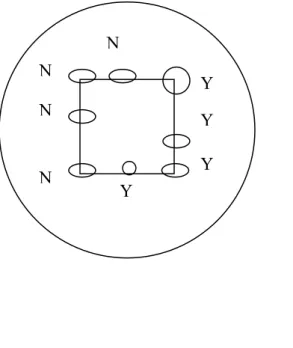
When counting random fields it is important to take a consistent approach to decide whether unicellular algal objects lying across the grid lines are counted in or out. A simple rule should be adopted as described in the CEN method (2006): unicellular algal cells crossing either the top or the left hand side of the grid are not counted whilst those crossing the bottom or right hand side of the grid are counted (Figure 4).

For filaments and colonies, only the cells or filament length that is inside the field of view should be counted – although these larger taxa should usually be counted at lower magnification in transects or full chamber count.

Figure 4 Example of rule for counting cells on edge of field

Y - counted N – not counted N N N N Y Y Y Y

(24)

23

Point to consider when counting

Algal objects and counting units:

Counting units are independent algal cells, colonies or filaments/trichomes. One species or taxa may be present in the sample as different counting units and may be counted at different magnifications.

For example, Microcystis colonies are counted in the whole-chamber or transect but individual Microcystis cells (which may be present if colonies are disintegrating) are counted in random fields. Similarly Dinobryon colonies may be counted in whole chamber or diameter transects, but single Dinobryon cells often need to be counted in random fields. Other examples of counting/algal units include:

− Colonies e.g. Aphanocapsa, Aphanothece, Coelomoron, Coelosphaerium, Cyanodictyon, Cyanonephron, Gomphosphaeria, Microcystis, Radiocystis, Snowella, Woronichinia, Coelosphaerium, Planktosphaeria, Sphaerocystis;

− Algal cells which can occur as single cells but also form colonies, e.g. Aulacoseira, Dinobryon, Melosira, are counted as cells;

− Colonies which have more or less permanent cell numbers, e.g. Desmodesmus/Scenedesmus (2, 4 or 8 cells), Pandorina (16 cells) Crucigenia (4 cells); − Filaments or trichomes e.g. Anabaena, Aphanizomenon, Oscillatoria, Planktothrix.

Species with a high variation of size can be counted in size-classes (e.g. Cryptomonadales <16 µm, 16-26 µm, >26 µm).

Calculating cells per colony/filament

It is often necessary to estimate the numbers of cells per colony or filament. For some taxa the cell numbers per colony may be consistent or have several modes as illustrated above whilst for others the cell numbers do not have a consistent distribution e.g. Microcystis where the number of cells per colony can vary from a few to several million cells.

o For estimating number of cells per colonies or coenobia:

Make direct counts of cells in the whole colony. If the colony is very large or cells

are very small, mean cell numbers may have to be estimated. This is best done by estimating cell numbers in a more restricted area or in ‘sub-colonies’ of the colony and estimating how many similar areas are contained within the counting field. These

(25)

24

can then be multiplied up by number of ‘sub-colonies’ or the ratio of small area to whole colony to get the total cell numbers, e.g. Microcystis, Woronichinia, etc.

o For estimating the number of cells per filament:

Make direct count of cells if it is possible. In other cases:

• Using filament measurements – for whole chamber or transect counts at low or intermediate magnification whole filament lengths can be measured for all filaments observed. If filaments are very abundant, mean dimensions can be estimated by measuring the length of at least 30 filaments. This could be done just once for each lake by both counters. For high-magnification random field of view or transect counts, only the length of the filaments lying within the grid should be measured.

• Using cell volumes – combine counting of filaments, with the mean numbers of cells per unit filament length, e.g. Aphanizomenon.

− If possible calculate the average number of cells per unit length from up to 10 filaments (e.g. 20 µm). This can be measured at a higher magnification if the cells are small or hard to distinguish easily (e.g. but for some species, like Planktothrix/ Oscillatoria this is not often possible);

− If you can differentiate cells, then the number of cells per filament is calculated by multiplying up the average filament length by the average number of cells per unit length.

• Where the algae form spiral filaments e.g. Anabaena circinalis, the average number of cells per gyre is counted and then the number of gyres per filament is estimated. The two numbers are multiplied together to give the estimated number of cells per filament.

Identification and coding

Species are coded as presented in the WISER_REBECCA taxa list for phytoplankton available on the WISER intranet. The present updated taxa list is also included in the counter spreadsheet.

Calculation of phytoplankton biovolume

Biovolumes must be measured for all taxa and is done by assigning simple geometric shapes toeach cell, filament or colony, measuring the appropriate dimensions and inputting these into formulae to calculate the cell volume. Available biovolumes can be used for taxa and different size-classes providing that taxa dimensions are checked during the analysis by measurements. This could be done just once for each lake by both counters.

(26)

25

The counting spreadsheet which will accompany this guidance includes a fixed, pre-determined, formula for the biovolume of each taxon. All that is required is for the appropriate mean dimensions to be input to the spreadsheet so that the biovolume can be calculated automatically (see points listed below).

Measurements of the required cell dimensions (length, width, diameter) are made at an appropriate magnification using a calibrated ocular eyepiece, e.g. a Whipple Graticule. The eyepiece is rotated so that the scale is put over the required cell dimension and the measurement made by taking the ocular measurement and multiplying by the calibration factor for that magnification and eyepiece combination. The measurements can be also made by image analysis.

Biovolume estimation of unicellular taxa

It is important to measure the linear dimensions of a number of individual units of all taxa observed in the sample. For taxa of more variable size (e.g. centric diatoms), and taxa that contribute significantly to the total biovolume (e.g. >5% of biovolume), at least 10

individuals should be measured.

For some species with external skeletons much larger than cell contents, e.g. Dinobryon, Urosolenia, the dimensions of the plasma/organic cell contents should be measured, not the external skeleton dimensions.

Biovolume estimation of filamentous taxa

For filamentous taxa, the average biovolume can be estimated using the method described in 0 for estimating number of cells per filament multiplying by the mean biovolume of one cell. Or it is possible to use the mean dimensions of filaments to calculate the biovolume of one filament multiplying by the number of filaments.

Biovolume estimation of colonial taxa

for colonial taxa, count or estimate cell numbers as described in 0 and multiply by mean cell dimensions (often single measure of dimensions needed). Using colony/coenobium measurements – measure colony width and depth e.g. Pediastrum – with colony depth approximated as an individual cell diameter.

(27)

26

A new CEN standard is under preparation for calculating cell volumes of phytoplankton. This CEN standard draft can be used to calculate biovolumes if less common taxa are added to the spreadsheet.

Data entry

An Excel spreadsheet will be provided for data entry. The counting can be carried out using different programmes or spreadsheets, but the final output should be transferred to the WISER Excel spreadsheet. The spreadsheet contains the whole WISER_REBECCA taxa list and provides biovolume formulae for many of the common taxa. It also allows the raw data to be summarised. All required details must be input into the counting spreadsheet according to the accompanying instructions.

Data to be entered will include information on the sample site (lake code, location, replicate and sub-sample no.) and date of collection, date of analysis, the person who carried out the count, information on the chamber and counting areas and the volume of sample used. For each taxa found, the number of units counted, the number of fields of view (or equivalent for whole chamber or diameter transects) in which it was counted and mean dimensions of the taxa will be recorded. For taxa which are counted in more than one form, e.g. individual cells and filaments/colonies, it is important to fill in one row for cells counted and the other for filaments or colonies. For filaments and colonies, an estimate of the numbers of cells is also usually required to calculate biovolume/ml. Cells/ml and biovolume/ml for each taxa are automatically calculated once the count and mean dimensions are entered.

Quality Assurance and validation of counts

Detailed quality assurance methodology and validation of counts are given in CEN (2006), NRA (1995), Kelly and Kelly & al. (1998) and Rott (1981, 2007). The following should be noted:

1) Details of microscopes, chambers (individually identified and calibrated) and calibration of all ocular/objective combinations should be recorded in a note book and kept for reference. If fixed volume pipettes these should be calibrated annually; 2) Checks for random distribution of sample should be done visually at low

magnification for each sample. Some simple checks include: comparing the number of observations in (a) half a chamber with the other half (b) comparing counts in the 1st transect with the 2nd transect and (c) comparing counts in the first 20 field of view with the next 20 fields. A more detailed check using simple Chi squared test should be done if a sample does not appear to be randomly sedimented or 1 sample every 3 months or so. The Chi squared test is not carried out in the WISER samples.

(28)

27

Literature - Methodology

CEN EN 15204, 2006. Water quality – Guidance standard for the routine analysis of phytoplankton abundance and composition using inverted microscopy (Utermöhl technique)

Kelly, M.G., 1998. Use of similarity measures in quality assurance of phytoplankton data. 7pp. Report to Environment Agency, Thames Region.

Kelly, M.G. & Wooff, D., 1998. Quality Assurance for Phytoplankton Data from the River Thames. 45pp. Report to Environment Agency, Thames Region

Lund, J.W.G.; Kipling, C. & LeCren, E.D., 1958. The inverted microscope method of estimating algal numbers and the statistical basis of estimations by counting. Hydrobiologia 11: 143-170.

National Rivers Authority, 1995. Test Methods and Procedures: Freshwater Phytoplankton. Biology Laboratory Procedures Manual. Peterborough: National Rivers Authority. SYKE. PL100 Quantitative and qualitative phytoplankton analysis. 12pp

Utermöhl, H., 1958. Zur Vervollkommnung der quantitativen Phytoplankton-Methodik. Mitteilungen der Internationale Vereinigung für Theoretische und Angewandte Limnologie 9: 1-38.

Rott, E., 1981. Some results from phytoplankton counting intercalibrations. Schweiz.Z.Hydrol. 43(1): 34-62.

Rott, E.; Salmaso N. & Hoehn E., 2007. Quality control of Utermöhl based phytoplankton biovolume estimates - an easy task or an Gordian knot? Hydrobiologia 578: 141-146.

Literature – taxonomic

This is not an exhaustive list of references on phytoplankton, but presents the documents currently used, to varying degrees, for the determination of phytoplankton taxa in lake surveys. The references highlighted are considered as less useful.

Anton, A.; Duthie, H. C., 1981. Use of cluster analysis in the systematics of the algal genus Cryptomonas, Canadian journal of botany, 59,6, 992-1002

Coesel, P. F. M.; Meesters, K. J., 2007. Desmids of the lowlands: Mesotaeniaceae and Desmidiaceae of the european lowlands, Zeist, NLD, KNNV Publishing. 351 p. Compère, P., 1986. Flore pratique des algues d'eau douce de Belgique : t.1 Cyanophyceae,

(29)

28

Compère, P., 1989. Flore pratique des algues d'eau douce de Belgique : t.2 Pyrrhophytes (Cryptophyceae, Dinophyceae), Raphidophytes (Raphidophyceae), Euglenophytes (Euglenophyceae), Meise, BEL, Jardin Botanique National de Belgique. 208 p.

Compère, P., 2001. Flore pratique des algues d'eau douce de Belgique : t.5 Desmidiees 1 Mesotaeniaceae, Gonatozygaceae, Peniaceae, Closteriaceae, Meise, BEL, Jardin Botanique National de Belgique. 69 p.

Czurda, V., 1932. Die Süßwasserflora Mitteleuropa Heft 9. Zygnemales, Jena, DEU, Verlag von Gustav Fischer. 232 p.

Dillard, G. E., 2000. Bibliotheca phycologica, band 106. Freshwater algae of the Southeastern United States: Part 7. Pigmented Euglenophyceae, Berlin, DEU, Cramer. 176 p.

Dillard, G. E., 2007. Bibliotheca phycologica, band 112. Freshwater algae of the souheastern United States: part. 8 Chrysophyceae, Xanthophyceae, Raphidophyceae, Cryptophyceae and Dinophyceae, Berlin, DEU, J. Cramer. 176 p.

Ettl, H., 1978. Süßwasserflora von Mitteleuropa 3. Xanthophyceae: 1. Teil, Stuttgart, DEU, Gustav Fischer Verlag. 530 p.

Ettl, H., 1983. Süßwasserflora von Mitteleuropa 9. Chlorophyta I: Phytomonadina, Stuttgart, DEU, Gustav Fischer Verlag. 807 p.

Ettl, H.; Gärtner, G., 1988. Süßwasserflora von Mitteleuropa 10. Chlorophyta II: Tetrasporales, Chlorococcales, Gloeodendrales, Stuttgart, DEU, Gustav Fischer Verlag. 807 p.

Förster, K.; Huber Pestalozzi, G., 1982. Die Binnengewässer, Band XVI. Das Phytoplankton des Süßsswassers: Systematik und Biologie: 8 Teil 1. Hälfte: Conjugatophycae, Zygnematales und Desmidiales (excl. Zygnemataceae), (e. Schweizebart'sche Verlagsbuchhandlung (nagele u obermiller) ed.), Stuttgart. 543 p.

Fott, B.; Huber Pestalozzi, G., 1972. Die Binnengewässer, Band XVI. Das Phytoplankton des Süßwassers: Systematik und Biologie: 6 Teil Chlorophyceae (Grunalgen) ordnung: Tetrasporales (E. Schweizerbart'sche Verlagsbuchhandlung ed.), Stuttgart, DEU. 150 Gemeinhardt, K., 1971. Dr L. Rabenhorst's Kryptogamen-Flora 12. Chlorophyceae 4.

Abteilung. Oedogoniales, New York, USA, Johnson reprint corporation. 453 p.

Gemeinhardt, K.; Schiller, J., 1971. Dr L. Rabenhorst's Kryptogamen-Flora 10. Flagellatae 2. Abteilung. Silicoflagellatae: Coccolithineae, New York, USA, Johnson reprint corporation. 589 p.

Huber Pestalozzi, G., 1969. Die Binnengewässer, Band XVI. Das Phytoplankton des Süsswassers: Systematik und Biologie: 4 teil Euglenophyceen, (E. Schweizerbart'sche Verlagsbuchhandlung ed.), Stuttgart, DEU. 606 p.

(30)

29

Huber Pestalozzi, G., 1976. Die Binnengewässer, Band XVI. Das Phytoplankton des Süsswassers: Systematik und Biologie: 2 teil 1 Halfte Chrysophyceen farblose flagellaten heterokonten, (E. Schweizerbart'sche Verlagsbuchhandlung ed.), Stuttgart, DEU. 365 p.

Huber Pestalozzi, G.; Fott, B., 1968. Die Binnengewässer, Band XVI. Das Phytoplankton des Süsswassers: Systematik und Biologie: 3 teil Cryptophyceae, Chloromonadophyceae, Dinophyceae 2. Auflage, (E. Schweizerbart'sche Verlagsbuchhandlung ed.), Stuttgart, DEU. 322 p.

Huber Pestalozzi, G.; Thienemann, A., 1942. Die Binnengewässer, Band XVI. Das Phytoplankton des Süsswassers: Systematik und Biologie: 2 Teil 2 Halfte Diatomeen, Stuttgart, DEU, E. Schweizerbart'sche Verlagsbuchhandlung. 549 p.

Huber Pestalozzi, G.; Thienemann, A., 1974. Die Binnengewässer, Band XVI. Das Phytoplankton des Süsswassers: Systematik und Biologie: 5 Teil Chlorophyceae (Grünalgen) Ordnung: Volvocales, (E. Schweizerbart'sche Verlagsbuchhandlung ed.), Stuttgart, DEU. 1300 p.

Javornicky, P., 2003. Taxonomic notes on some freshwater planktonic Cryptophyceae based on light microscopy, Hydrobiologia, 502, 1-3, 271-283.

John, D. M.; Brook, A. J.; Whitton, B. A., 2002. The Freshwater Algal Flora of the British Isles. An Identification Guide to Freshwater and Terrestrial Algae., (Cambridge University Press ed.), Cambridge. 702 p.

Joosten, A. M., 2006. Flora of the Blue-green Algae of the Netherlands, Volume 1: The non-filamentous species of inland waters. 240 p.

Kadlubowska, J. Z., 1984. Süßwasserflora von Mitteleuropa 16. Chlorophyta VIII: Conjugatophyceae I: Zygnemales, Jena, DEU, VEB Gustav Fischer Verlag. 531 p. Kolkwitz, R.; Krieger, H., 1971. Dr L. Rabenhorst's Kryptogamen-Flora 13. 2. Abteilung.

Zygnemales: Lieferung 1-4, New York, USA, Johnson reprint corporation. 163 p. Komarek, J.; Anagnostidis, K., 1999. Süßwasserflora von Mitteleuropa 19. Cyanoprokaryota

1.Teil: Chroococcales, (Gustav Fischer ed.), Stuttgart, Gustav Fischer. 548 p.

Komarek, J.; Anagnostidis, K., 2005. Süßwasserflora von Mitteleuropa 19. Cyanoprokaryota 2.Teil: Oscillatoriales, (Elsevier SpeKtrum Akademischer Verlag ed.), München, Elsevier. 759 p.

Komarek, J.; Fott, B.; Huber Pestalozzi, G., 1983. Die Binnengewässer, band XVI. Das phytoplankton des susswassers systematik und biologie: 7 teil 1 Halfte Chlorophyceae (Grunalgen) ordnung: Chlorococcales, (E. Schweizerbart'sche verlagsbuchhandlung ed.), Stuttgart, DEU. 1044 p.

(31)

30

Komarek, J.; Zapomelova, E., 2007. Planktic morphospecies of the cyanobacterial genus Anabaena = subg. Dolichospermum - 1. part: coiled types, Fottea, 7,1, 1-31.

Komarek, J.; Zapomelova, E., 2008. Planktic morphospecies of the cyanobacterial genus Anabaena = subg. Dolichospermum - 2. part: straight types, Fottea, 8,1, 1-14.

Krammer, K.; Lange Bertalot, H., 1991. Süßwasserflora von Mitteleuropa 2. Bacillariophyceae 3. Teil: Centrales, Fragilariaceae, Eunotiaceae, Stuttgart, Gustav Fischer Verlag. 576 p.

Krammer, K.; Lange Bertalot, H., 1999. Süßwasserflora von Mitteleuropa 2. Bacillariophyceae 1. Teil: Naviculaceae, Berlin, Allemagne, Specktrum Akademischer Verlag GmbH Heidelberg. 876 p.

Krammer, K.; Lange Bertalot, H., 2000. Süßwasserflora von Mitteleuropa 2. Bacillariophyceae Part 5: English and French translation of the keys, Berlin, DEU, Spektrum. 311 p.

Krammer, K.; Lange Bertalot, H., 2004. Süßwasserflora von Mitteleuropa 2. Bacillariophyceae 4 Teil: Achnanthaceae Kritische Ergänzungen zu Achnanthes s.l., Bavicula s. str., Gomphonema, Berlin, DEU, Spektrum. 468 p.

Krammer, K.; Lange Bertalot, H., 2007. Süßwasserflora von Mitteleuropa 2. Bacillariophyceae 2. Teil : Bacillariaceae, Epithemiaceae, Surirellaceae, Munich, DEU, Elsevier. 610 p.

Krieger, W., 1937. Dr L. Rabenhorst's Kryptogamen-Flora 13. Conjugatae 1. Abteilung. Die desmidiaceen 1. Teil, New York, Johnson reprint corporation. 808 p.

Krieger, W., 1939. Dr L. Rabenhorst's Kryptogamen-Flora 13. 1. Abteilung. Die desmidiaceen 2. Teil Lieferung 1, New York, Johnson reprint corporation. 163 p. Kristiansen, J.; Preisig, H. R., 2007. Süßwasserflora von Mitteleuropa 1. Chrysophyte and

haptophyte algae: Part 2: Synurophyceae, (2° ed.), Berlin, DEU, Spektrum Akademisher Verlag. 252 p.

Lenzenweger, R., 1996. Bibliotheca phycologica, band 101. Desmidiaceenflora von Österreich. Teil 1, Berlin, DEU, Cramer. 162 p.