HAL Id: hal-02269391
https://hal.archives-ouvertes.fr/hal-02269391
Submitted on 20 May 2020
HAL is a multi-disciplinary open access
archive for the deposit and dissemination of
sci-entific research documents, whether they are
pub-lished or not. The documents may come from
L’archive ouverte pluridisciplinaire HAL, est
destinée au dépôt et à la diffusion de documents
scientifiques de niveau recherche, publiés ou non,
émanant des établissements d’enseignement et de
Totally Balanced Dissimilarities
François Brucker, Pascal Prea, Célia Châtel
To cite this version:
François Brucker, Pascal Prea, Célia Châtel. Totally Balanced Dissimilarities. Journal of
Classifica-tion, Springer Verlag, 2019, �10.1007/s00357-019-09320-w�. �hal-02269391�
Totally balanced dissimilarities
Fran¸cois Brucker, Pascal Pr´ea and C´elia Chˆatel
´
Ecole Centrale Marseille LIF, CNRS UMR 7279
38 rue Joliot-Curie - F-13451 Marseille Cedex 20, France. email: [email protected]
email: [email protected] email: [email protected]
Abstract. We show in this paper a bijection between totally balanced hy-pergraphs and so called totally balanced dissimilarities. We give an efficient way (O(n3) where n is the number of elements) to (i) recognize if a given dissimilarity is totally balanced and (ii) approximate it if it is not the case. We also introduce a new kind of dissimilarity which generalize chordal graphs and allows a polynomial number of cluster that can be easily computed and interpreted.
June 26, 2017 – 16:26
1
Introduction
Totally balanced hypergraphs, initially defined by Lovasz (1968), is a hy-pergraph structure which corresponds to the notion of tree for graphs (see Lehel, 1985) thus occurring in various applications like linear programming, databases structures of phylogenetic problems.
Totally balanced hypergraphs are equivalent to Γ -free 0/1-matrices (Antsee and Farber, 1984), strongly chordal graphs (Farber, 1983) or dismantlable lattices (Brucker and G´ely, 2010). These alternative characterizations make them a good classification model because their clusters can be interpreted ei-ther as a sup of two elements (dismantlable lattice) or as a maximal clique of some graph (strongly chordal graph), and the whole structure is linked by an underlying family of trees. Moreover, they admit a convenient graphical rep-resentation (Brucker and Pr´ea, 2015). Finally totally balanced hypergraphs are weak-hierarchies (Brucker and G´ely, 2010 — see Bandelt and Dress (1989) for a definition of weak-hierarchies), they have a lot of good practical prop-erties (see Bertrand and Diatta, 2014 for instance) like admitting a relatively small number of overlapping clusters (at most the square of the number of elements) or being equivalent to an underlying metric model.
We will characterize in this paper the set of dissimilarities, named totally balanced dissimilarities, whose cluster set is a totally balanced hypergraph.
This characterization will also allow us to give new demonstrations of some well known theorems for graphs and to generalize them to dissimilarities.
We will also give three polynomial algorithms (in O(n3) operations where n is the number of elements) for dealing with those dissimilarities: one to check if a given dissimilarity is totally balanced, one to approximate (if nec-essary) a given dissimilarity into a totally balanced dissimilarity and the last one to give all the clusters associated with a totally balanced dissimilarity.
This paper is organized as follows. Section 2 gives a definition of totally balanced dissimilarities and shows that they are in bijection with totally balanced hypergraphs. Section 3 gives an efficient way of determining the clusters of those dissimilarities by using a new kind of dissimilarities (chordal dissimilarities). We then show an algorithm for determining if a given dis-similarity is totally balanced (Section 4) and a way to approximate it if it is not the case (Section 5). We finally give an example of the use of these algorithms on a real dataset (Section 6).
2
Totally Balanced Structure correspondances
We will define in this section totally balanced hypergraphs through a linear order, named totally balanced order. Moreover, this order will be used to link the different totally balanced structures (hypergraphs: Proposition 3, dissim-ilarities: 5 and binary matrices: Proposition 13). Finally, we define totally balanced dissimilarities and prove that there is a bijection between totally balanced hypergraphs and the cluster hypergraphs of those dissimilarities (Proposition 6).
2.1 Hypergraphs
Recall that an hypergraph is a couple H = (V, E) where E ⊆ 2V. As for a graph, elements of V and E are named vertices and edges respectively. We will also denote by H the closure of H: H = (V, E) where E is the closure by intersection of E (E is the smallest subset of 2V such that E ⊆ E and X, Y ∈ E =⇒ X ∩ Y ∈ E ∨ X ∩ Y = ∅) and by H|W the restriction of H to W ⊂ V : H|W = (W, E|W), where E|W = {X ∩W | X ∈ E, X ∩W 6= ∅}. A sequence (v1, e1, . . . , vk, ek) where vi ∈ V and ei ∈ E (1 ≤ i ≤ k) is a path in H if vi, vi+1 ∈ ei. A cycle is a path (v1, e1, . . . , vk, ek) with v1 ∈ ek. Moreover, a cycle (v1, e1, . . . , vk, ek) is a special cycle if k ≥ 3 and vi ∈ ej if and only if j = i, j = i − 1 or (i, j) = (1, k).
An hypergraph is totally balanced if it has no special cycle. This can be seen as the hypergraph version of trees (a graph with no cycle). We have the two elementary properties:
Proposition 1. An hypergraph H = (V, E) is totally balanced if and only if its closure is totally balanced.
Proposition 2. If an hypergraph H = (V, E) is totally balanced then for all X, Y, Z ∈ E: X ∩ Y ∩ Z ∈ {X ∩ Y, Y ∩ Z, X ∩ Z}
Let H = (V, E) a hypergraph. A linear order v1 < v2 < · · · < vn on V is totally balanced (with H) if the sets {X | vi ∈ X, X ∈ E|vi,...,vn} are chains
for all 1 ≤ i ≤ n. A set C ⊂ 2V is a chain if for all X, Y ∈ C, either X ⊆ Y or Y ⊆ X.
Proposition 3 (Brucker and Gely, 2010). An hypergraph H is totally balanced if and only if it admits a totally balanced ordering.
2.2 Dissimilarities
A dissimilarity on a set V is a function d from V × V to the non-negative real numbers which is symmetrical (d(x, y) = d(y, x)) and admits a zero-diagonal (d(x, x) = 0). All the dissimilarities occurring in this paper will be assumed to be proper: d(x, y) = 0 ⇐⇒ x = y.
For σ ≥ 0, the threshold graph Gσ of d admits V as a vertex set and the pairs xy such that d(x, y) ≤ σ as edge set. The maximal cliques of the threshold graphs are called clusters. For σ ≥ 0 and x ∈ V , the ball B(x, σ) is the set {y ∈ V : d(x, y) ≤ σ}. Given a dissimilarity d on V one can associate two hypergraphs:
• its cluster hypergraph C(d) = (V, E) where E is the set of all its clusters (the maximal cliques for all its threshold graphs),
• its ball hypergraph B(d) = (V, E) where E is the set of all the balls of d. The diameter of a set X ⊆ V is equal to diam(X) = max{d(x, y) | x, y ∈ X}. The diameter of a set X is the smallest α for which X is a clique of the threshold graph Gα.
We define then the totally balanced dissimilarities as the dissimilarities for which C(d) is totally balanced. An order v1, . . . vn is said to be totally balanced with d if it is totally balanced with C(d).
Given dissimilarity d on V , we say that v1, . . . , vn is a chordal order for d if for all i ≤ j, k, d(vj, vk) ≤ max{d(vi, vj), d(vi, vk)}. A dissimilarity is said to be chordal if it admits a chordal order.
Note that for a given totally balanced dissimilarity d, the totally balanced orders of d are chordal orders. Proposition 4 characterize the chordal orders that are also totally balanced.
Proposition 4. An order v1 < · · · < vn on V is totally balanced for a dissimilarity d on V if and only if:
1. it is a chordal order,
2. for all (g, h, i, j, k) with g, h ≤ i < j, k: either d(vg, vk) ≤ max{d(vg, vi), d(vg, vj)}, or d(vh, vj) ≤ max{d(vh, vi), d(vh, vk)}.
Proof. First suppose that the order is totally balanced for C(d) but not chordal for d. Then there exist i < j, k such that d(vj, vk) > max{d(vi, vj), d(vi, vk)}; so there exists two maximal cliques X and Y of the threshold graph Gmax{d(vi,vj),d(vi,vk)}
such that X contains vi and vj but not vk and Y contains vi and vk but not vj. Thus the order cannot be totally balanced for C(d).
Second suppose that the order it totally balanced and chordal but there exist g, h ≤ i ≤ j, k such that d(vg, vk) > max{d(vg, vi), d(vg, vj)}, and d(vh, vj) > max{d(vh, vi), d(vh, vk)}. So there exists a maximal clique X of the threshold graph Gmax{d(vg,vi),d(vg,vj)} containing g, i and j (because the
order is chordal) but not k and a maximal clique Y of the threshold graph Gmax{d(vh,vi),d(vg,vk)}containing g, i and k (because the order is chordal) but
not j. So the order cannot be totally balanced for C(d).
Consequently, if v1< · · · < vn on V is totally balanced for C(d) then the two conditions are satisfied.
Conversely, we suppose that the order is not totally balanced for C(d). Let i be an index such that {Z | vi ∈ Z, Z ∈ C(d)|vi,...,vn} is not a chain.
There exist j, k > i and X, Y in C(d) such that vj ∈ X \ Y and vk ∈ Y \ X. We suppose with no loss of generality that the diameter of X is not smaller than the diameter of Y .
Since X and Y are maximal cliques of some threshold graphs of d, there exists vg ∈ X and vh ∈ Y such that d(vg, vk) > diam(X) and d(vh, vj) > diam(Y ). In addition, vg ∈ X \ Y and vh∈ Y \ X (otherwise, we would have X ⊂ Y or Y ⊂ X).
If the order is not chordal the property is verified. We suppose now that the order is chordal. We will prove that the second condition of the property is not satisfied.
Since the diameter of X is not smaller than the diameter of Y we have that g < i; otherwise, we would have d(vg, vk) ≤ max{d(vi, vg), d(vi, vk)} ≤ max{diam(X), diam(Y )} ≤ diam(X).
If h < i, then the second condition is not satisfied for the 5-tuple (g, h, i, j, k). If i < h, d(vh, vj) ≤ max{d(vi, vh), d(vi, vj)}. As d(vi, vh) ≤ diam(Y ) < d(vh, vj), we have d(vh, vj) ≤ d(vi, vj) and d(vi, vj) > diam(Y ). So, there exist vg0 ∈ X such that d(vg0, vh) > diam(X)}. In addition, g0< i (otherwise,
we would i < g0, h and d(vg0|,v
h > max{d(vi, vh), d(vi, vg0}). Thus the second
property is not verified for the 5-tuple (g0, i, i, j, h). u
Graphs whose maximal cliques hypergraph C(G) is totally balanced have been characterized by Farber (1983). They are known as the strongly chordal graphs, which are a subclass of chordal graphs.
A graph is said to be chordal if every cycle x1x2. . . xnx1 with n ≥ 3 admits a chord (an edge xixj with i < j + 1). They can be characterized by the existence of simplicial ordering v1, . . . , vn of the vertices, i.e. an ordering such that for all i < j, k, if vivj and vivk are edges then vjvk is also an edge (Dirac, 1961).
Since a graph G = (V, E) can be seen as a dissimilarity dGon V (dG(x, y) = 1 if xy ∈ E and dG(x, y) = 2 otherwise), chordal orders for dissimilarities are a direct generalization of simplicial orderings, and dissimilarities admitting a chordal order a direct generalization of chordal graphs.
It is known that B(dG) is totally balanced if and only if C(dG) is totally balanced (Farber, 1983). This is no more true for (general) dissimilarities for which we only have an implication as proved by Proposition 5 and the counter example of Table 1.
Proposition 5. For a given dissimilarity d on V , if B(d) admits v1< · · · < vn as a totally balanced order then it is also a totally balanced order for C(d). Proof. Let v1< · · · < vnbe a totally balanced order for B(d). Let vi, vj, vkbe three elements of V such that vi< vj, vk. If d(vj, vk) > max{d(vi, vj), d(vi, vk)}, we would have vk ∈ B(vj/ , d(vi, vj)) and vj∈ B(vi, d(vi, vk)). As vi/ is in these two balls, the order would not be totally balanced for B(d). So Condition 1 of Property 4 is verified.
Let (g, h, i, j, k) be a 5-tuple not verifying Condition 2 of Property 4. We
would have vk ∈ B(vg, max{d(vg, vi), d(vg, vj)}) and vj/ ∈ B(vh, max{d(vh, vi), d(vh, vk)})./ As vi is in these two balls, the order would not be totally balanced order for
B(d). u t
Table 1: A dissimilarity d for which C(d) is totally balanced (admits x < y < z < t as a totally balanced order) but B(d) is not ((z, B(z, 2), x, B(y, 2), y, B(t, 1)) is a special cycle).
x 0 y 2 0 z 2 3 0 t 2 1 1 0
2.3 Bijections
The bijection between totally balanced hypergraphs and totally balanced dissimilarities is a special case of one of the general bijections of Bertrand (2000). One can associate to a given a hypergraph H = (V, E) a valuation f from E to R+. The couple (H, f ) is said to be a valued hypergraph. The valuation f is said to be a strict index if if X ( Y implies f (X) < f (Y ). Note that the cardinal of a cluster is a strict index for any hypergraph and the diameter is a strict index of C(d) for any dissimilarity d.
Theorem 1 (Bertrand, 2000). Let H = (V, E) be an hypergraph contain-ing the scontain-ingletons and V as edges and such that for any edges X, Y, Z, we have X ∩ Y ∩ Z ∈ {X ∩ Y, Y ∩ Z, X ∩ Z} and let f be a strict index of H such that f ({x}) = 0 for all x ∈ V . Then the dissimilarity d on V defined by d(x, y) = min{f (X)|X ∈ E, x, y ∈ X} is such that:
• C(d) = E
• for all X ∈ E, f (X) is the diameter of X for d As a direct consequence, we have:
Proposition 6. Let H = (V, E) be a totally balanced hypergraph containing the singletons and the whole set as edges, and let f be a strict index of H. Then the dissimilarity d defined by d(x, y) = min{f (X)|X ∈ E, x, y ∈ X} is such that C(d) = E.
Conversely, for any totally balanced dissimilarity d on V :
• (V, C(d)) is a totally balanced hypergraph containing the singletons and the whole set as edges.
• The diameter is a strict index on (V, C(d)).
3
Clusters
In the general case, a dissimilarity on a n-set can have an exponential number of clusters. We will show in this section that a chordal dissimilarity have at most n2 clusters. Moreover, we will give an O(n3) algorithm to compute them. This algorithm is linear in the size of the output in the worst case (O(n2) clusters, each of size O(n)). Since totally balanced dissimilarities are a subset of chordal dissimilarities, this also gives a linear algorithm (in the worst case) for finding the clusters of totally balanced dissimilarities. Proposition 7. Let d be a dissimilarity on V admitting v1< · · · < vn as a chordal order, then for every X ∈ C(d), X = B(v∗, α)|{v≥v∗} where:
• v∗ is the smallest element of X (according to the chordal order). • α is the diameter of X (according to d).
Proof. If v, w ∈ B(v∗, α)|{v≥v∗} then d(v, w) ≤ max{d(v∗, v), d(v∗, w)} ≤ α
(the order is chordal). So the truncated ball B(v∗, α)|{v≥v∗} is a clique of
diameter α.
Moreover, by construction, the maximal clique X is included in B(v∗, α)|{v≥v∗}.
Thus X = B(v∗, α)|{v≥v∗}.
u t
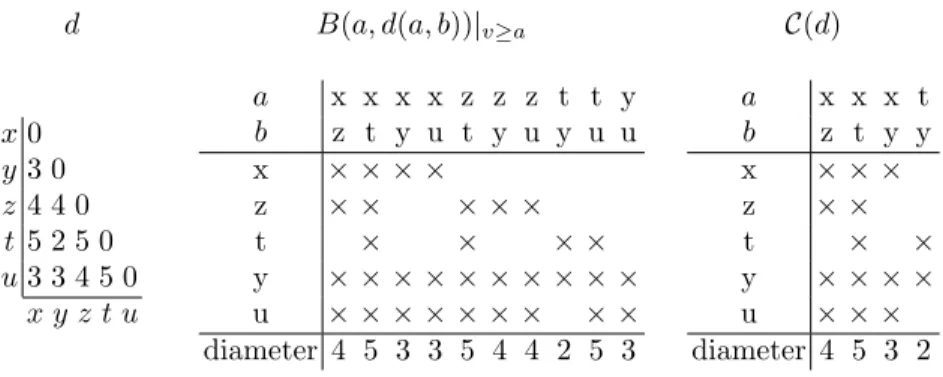
Proposition 7 shows that the maximal cliques of d are truncated balls, i.e. C(d) ⊆ {B(v, d(v, w))|{x≥v}| v ≤ w}. The number of clusters is then bounded by O(|V |2). Table 2 shows a dissimilarity with its truncated balls and maximal cliques.
Table 2: A totally balanced dissimilarity d admitting x < z < t < y < u as a chordal order.
d B(a, d(a, b))|v≥a C(d)
x 0 y 3 0 z 4 4 0 t 5 2 5 0 u 3 3 4 5 0 x y z t u a x x x x z z z t t y b z t y u t y u y u u x × × × × z × × × × × t × × × × y × × × × × × × × × × u × × × × × × × × × diameter 4 5 3 3 5 4 4 2 5 3 a x x x t b z t y y x × × × z × × t × × y × × × × u × × × diameter 4 5 3 2
Proposition 8. Let d be a dissimilarity on V admitting v1 < · · · < vn as a chordal order. The truncated ball B(vi, d(vi, vj))|{v≥vi} with i ≤ j is a
maximal clique with diameter d(vi, vj) if for all vk < vi: max{d(vk, vi), d(vk, vj)} = d(vi, vj) =⇒
Card(B(vk, d(vi, vj))|{v≥vi}) < Card(B(vi, d(vi, vj))|{v≥vi})
Proof. Note α = d(vi, vj). According to Proposition 7, the truncated ball Bi = B(vi, α)|{v≥vi} is a clique. It is maximal if it is not included in another
clique of same diameter, i.e. if there does not exist a truncated ball Bk = B(vk, α)|{v>vk} with vk < vi such that Bi⊂ Bk.
If it is the case, d(vk, vi) ≤ α and d(vk, vj) ≤ α. As the orded is chordal, d(vi, vj) ≤ max{d(vk, vi), d(vk, vj)}. So α = max{d(vk, vi), d(vk, vj)}.
Let vl> vi be an element of Bk, d(vi, vl) ≤ max{d(vk, vi), d(vk, vl} ≤ α. So Bk|{v≥vi}⊆ Bi|{v≥vi}. Clearly, Bi|{v≤vi}⊆ Bk|{v≤vi}. So, Bi⊆ Bk if and
only if Card(Bi) < Card(Bk|{v≥vi})
u t
Algorithm 1 uses propositions 7 and 8 to compute the clusters of a dissimi-larity, one of its chordal orders being given. It iterates over all the possible balls according to the chordal order and keeps those which are clusters. To do that task efficiently, the algorithm maintains numbers Sk(t) for 1 ≤ k, t ≤ n which are defined by:
• At step i, if there exist a truncated ball Bk(α) = B(vk, α)|v>vk such that Card(Bk(α)|v>vi) = t, then Sk(t) = α. Notice that, since Bk(α) is a
truncated ball, there is at most one Bk(α) with t elements. • At Step i, if no such truncated ball exists, Sk(t) = −1.
By proposition 8, a given truncated ball Cij = B(vi, d(vi, vj))|{v≥vi}with i ≤
j is a maximal clique if it does not exist k < i such that d(vk, vi) ≤ d(vi, vj) and Sk(|Cij|) = d(vi, vj).
The numbers Sk(t) allow us to check efficiently (in O(|V |)) the conditions of Proposition 8. So we have the following proposition 9.
Proposition 9. For a given chordal dissimilarity d and a chordal order v1< · · · < vn, Algorithm 1 returns the set C(d) in O(|V |3) operations and size.
4
Recognition
We will give in this section an O(|V |3) algorithm to determine if a given dissimilarity d on V is chordal or totally balanced. This algorithm first check whether a given dissimilarity is chordal or not by finding one of its chordal orders (Algorithm 2). We then compute its cluster hypergraph and its associ-ated binary matrix. We linearly check (Spinrad, 2003) that its doubly lexical ordering is Γ -free.
4.1 Chordal orders
Finding a chordal order for a given dissimilarity d can be iteratively done using Proposition 10.
Proposition 10. If a dissimilarity d on a set V admits a chordal order then for all x ∈ V such that ∀y, z ∈ V d(y, z) ≤ max{d(x, y), d(x, z)}, the restriction of d on V \{x} admits a chordal order.
Proof. If d admits a chordal order v1 < v2 < · · · < vn, then v2 < . . . < vn is a chordal order on {v2, . . . vn}. If there exits vi such that or all y, z ∈ V , d(y, z) ≤ max{d(vi, y), d(vi, z)}, then vi< v1< · · · < vi−1< vi+1< · · · < vn is also a chordal order for d.
u t
Algorithm 2 uses then Proposition 10 iteratively to find a chordal order for a given dissimilarity d.
Algorithm 1: Cluster-Set-Construction
Data: A dissimilarity d on a n-set V and one of its chordal order v1< · · · < vn
Result: The cluster set C(d) // Initialization
1 C ← ∅
2 S1(t) ← −1 for 1 ≤ t ≤ n
// All the balls with center v1 are clusters 3 for j ← 1 to n do 4 add B(v1, d(v1, vj)) to C 5 S1(|B(v1, d(v1, vj))| − 1) ← d(v1, vj) // Main Loop 6 for i ← 2 to n do 7 Vi← {vi, . . . , vn} 8 Si(t) ← −1 for all 1 ≤ t ≤ n 9 for j ← i to n do
10 Cij ← B(vi, d(vi, vj)) ∩ Vi
11 if @k < i such that (d(vk, vi) ≤ d(vi, vj) and Sk(|Cij|) = d(vi, vj)) then
// Cij is not included in a cluster with same diameter: its a cluster
12 add Cij to C 13 Si(|Cij| − 1) ← d(vi, vj) // Update Sizes 14 for j ← 1 to i − 1 do 15 for t ← 1 to n do 16 if Sj(t) ≥ d(vj, vi) then 17 if t > 1 and Sj(t − 1) = −1 then 18 Sj(t − 1) ← Sj(t) 19 Sj(t) ← −1 20 return C
Proposition 11. Given a dissimilarity d on V , Algorithm 2 returns a chordal order (if there exists one) in O(|V |3) operations.
Proof. At each step, Ni(v) is the number of pairs {x, y} ⊂ Vi for which d(x, y) > max{d(v, x), d(v, y)}. By Proposition 10, Algorithm 2 return a chordal order. Clearly, it runs in O(|V |3) operations.
u t
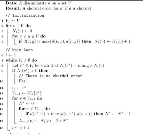
Algorithm 2: Chordal-Order-Construction Data: A dissimilarity d on a set V
Result: A chordal order for d, if d is chordal // Initialization
1 V1← V 2 for v ∈ V do 3 N1(v) ← 0 4 for x 6= y ∈ V do
5 if d(x, y) > max{d(v, x), d(v, y)} then N1(v) ← N1(v) + 1 // Main Loop
6 i ← 1
7 while Vi6= ∅ do
8 Let v∗∈ Vi be such that Ni(v∗) = minv∈ViNi(v) 9 if Ni(v∗) > 0 then
// There is no chordal order 10 Fail 11 vi← v∗ 12 Vi+1 ← Vi\{v∗} 13 for v ∈ Vi+1 do 14 N∗← 0 15 for w ∈ Vi+1 do 16 if d(v∗, w) > max{d(v, v∗), d(v, w)} then N∗← N∗+ 1 17 Ni+1(v) ← Ni(v) − 2 ∗ N∗ 18 i ← i + 1 19 return v1< · · · < vn
Table 3 shows the progression of the different Niwhen computing the chordal order x < z < t < y < u for the dissimilarity d of Table 2.
Table 3: Values for Ni when computing the chordal order x < z < t < y < u for the dissimilarity d of Table 2.
N1 N2N3 N4 N5 x 0 z 0 0 t 0 0 0 y 6 4 2 0 u 0 0 0 0 0
4.2 Totally balanced orders and Γ -free matrices
Finding a totally balanced order can be done using the equivalence between totally balanced hypergraphs and Γ -free matrices.
A n×m binary matrix M is equivalent to a hypergraph H(M ) = ({1, . . . , n}, {C1, . . . , Cm}) where Cj = {i | Mi,j = 1} (1 ≤ j ≤ m). Conversely, given a hypergraph H = (V, E), if we label V as {v1, . . . , vn} and E as {e1, . . . , em}, H is equivalent to a n×m binary matrix M(H) where M(H)i,j= 1 whenever vi ∈ ej.
We will say that a binary matrix M is totally balanced if H(M ) is totally balanced. A n × m binary matrix M is said to be Γ -free whenever for any 1 ≤ i < i0 ≤ n and any 1 ≤ j < j0 ≤ m: Mi,j = Mi,j0 = Mi0
,j = 1 implies Mi0,j0 = 1. A Γ -free ordering of a matrix M is an ordering of its lines and
columns such that M (when re-ordered) is Γ -free.
A doubly lexical ordering of an n × m binary matrix is an ordering of its lines and columns such that if the rows and columns are viewed as n or m digit numbers read from right to left for lines and from bottom to top for columns, both rows and columns occur in increasing order. Every binary matrix admits a doubly lexical ordering. Doubly lexical orderings, Γ -free matrices and totally balanced matrices are linked by Theorem 2.
Theorem 2 (Antsee and Farber, 1984). Given a binary matrix M , the three following assertions are equivalent:
1. M is a totally balanced binary matrix,
2. There is a doubly lexical ordering of M which is Γ -free, 3. Every doubly lexical ordering of M is Γ -free.
By Theorem 2, determining if a hypergraph H is totally balanced can be done by doubly lexical order M(H) and determine if this ordering is Γ -free. Finding a doubly lexical ordering of a binary matrix and determining if this ordering is Γ -free can be done by two algorithms of Spinrad. Given a n × m binary matrix M , Spinrad (1993) gives a linear algorithm (in O(nm) operations) which returns a doubly lexical ordering of M . The matrix M is then totally balanced if the ordering is also Γ -free, which can also be checked (and approximated by adding 1 to avoid Γ ’s if necessary) in O(nm) operations. See for instance Spinrad (2003) for a description of these three algorithms (the doubly lexical ordering, the check if a given matrix admits a Γ and the approximation into a Γ -free matrix).
The above algorithms give a O(|V | · |E|) operations and space procedure to determine whether a given hypergraph H = (V, E) is totally balanced by checking if a doubly lexical ordering of M(H) is Γ -free. Since, by Proposi-tion 2, a totally balanced hypergraph cannot have more than (|V |2+ |V |)/2 clusters, this is also a O(|V |3) time and space algorithm.
Finally, Propositions 12 and 13 show that this will also lead to find the totally balanced orders of a totally balanced hypergraph. These two propo-sitions link Γ -free and totally balanced orderings.
Proposition 12. If a n × m binary matrix M is Γ -free, the natural order of its lines (1, 2, . . . , n) is totally balanced for H(M ).
Proof. Let M be a Γ -free matrix, and i, j, j0 be such that j < j0 and Mi,j= Mi,j0 = 1. If Mi0,j = 1 with i0 ≥ i, then Mi0,j0 = 1. Thus Cj∩ {i, . . . , n} ⊆
Cj0 ∩ {i, . . . , n} if i ∈ Cj∩ Cj0 and j ≤ j0, i.e. the order 1, 2, . . . , n is totally
balanced for H(M ). u
t
Proposition 13. If the order v1 < · · · < vn is totally balanced for H = (V, E), then there exists a Γ -free column ordering for M(H) where line i corresponds to vi.
Proof. For X and Y in E, we denote by VXY the set {viXY, viXY+1, . . . , vn}
where iXY = min{i | vi ∈ X ∩ Y }. If X ∩ Y = ∅, iXY does not exist and we define VXY = ∅. We consider the directed graph G with E as vertex set and such that (X, Y ) is an arc (we denote it by X → Y ) if X ∩ VXY ( Y ∩ VXY. Notice that, if X → Y , then VXY 6= ∅ (the converse is false).
We now proof that if X → Y and Y → Z, then X → Z or iXY < iY Z. Suppose that iXY ≥ iY Z. In this case, viXY ∈ Z ∩ X, thus iXZ exists;
moreover iXZ ≤ iXY. As X → Y , there exists j > iXY such that vj ∈ Y \ X. As Y → Z and iY Z ≤ iXY, vj ∈ Z \ X. As the order is totally balanced, X ∩VXZis included in, equal to or contains Z ∩VXZ. As vj∈ VXZ, X ∩VXZ( Z ∩ VXZ and X → Z.
So the directed graph G is acyclic and its vertex set admits a topological order <T (if Xi → Xj then i <T j). Ordering the columns of M(H) along <T and the lines by the totally balanced order of H makes the matrix M(H) Γ -free.
u t
4.3 Recognition procedure
Putting together the preceding parts, we get a simple algorithm which rec-ognize in time O(|V |3) if a given dissimilarity d on V is totally balanced or not:
Step 1 of Algorithm 3 is Algorithm 2. Step 4 is Algorithm 1. Both steps run in O(n3). Since the matrix M(C(d)) has n lines and n2 columns, the test on line 6 also runs in O(n3).
A doubly lexical order of the dissimilarity in Table 2 is presented in Ta-ble 4. The matrix is Γ -free: the dissimilarity of TaTa-ble 2 is totally balanced.
Algorithm 3: Check-Totally-Balanced-Dissimilarity Data: A dissimilarity d on a n-set V
1 Try to find a chordal order 2 if @ chordal order then
3 return “d is not chordal thus not totally balanced” 4 Compute M(C(d))
5 Order M(C(d)) along a doubly lexical order 6 if M(C(d)) is Γ -free then
7 return “d is totally balanced” 8 else
9 return “d is chordal but not totally balanced”
Table 4: Doubly lexical ordering of the binary matrix of Table 2. a t x x x b y y z y t × × z × × x × × × u × × × y × × × × diameter 2 3 4 5
5
Approximation
We present in this section a O(|V |3) time and space procedure to approximate a dissimilarity d on V by a totally balanced one. If the initial dissimilarity is already totally balanced, the resulting dissimilarity will be the same. This procedure can be sketched as follows:
1. Approximate d into a chordal dissimilarity d0 (See Section 5.1).
2. Compute M(d0) and approximate it into a Γ -free matrix M0 (See Sec-tion 5.2).
3. Associate a totally balanced dissimilarity to the valued n × m matrix (M0, (αi)1≤i≤m) where the valuations (αi)1≤i≤m come from d0( See Sec-tion 5.3).
5.1 Approximation by a chordal dissimilarity
In order to approximate a given dissimilarity d on V , one can proceed in two steps:
1. Find a possible linear order on V .
2. Approximate d into a dissimilarity chordally compatible with the chosen order.
Finding a potential order can be done using Section 4.1. Since the origi-nal dissimilarity may not be chordal, we have to remove in Algorithm 2 the check whether Nd(v∗) equals 0 or not. If we keep at each step an element v∗ which realizes the minimum of Nd(), we are assured that the algorithm will always return a linear order on V and that this order is chordal if d is chordal. Let then d be a dissimilarity on V and v1 < · · · < vn an order on V . One can then use Algorithm 4 which approximate the dissimilarity d into a dissimilarity d0 which admits this order as a chordal one.
Algorithm 4: Chordal-Approximation-According-To-Order Data: A dissimilarity d on a n-set V and a linear order v1< · · · < vn
on V
Result: A dissimilarity d0 admitting v1< · · · < vn as chordal order. 1 d0 ← d
2 for i ← 1 to n do 3 for j ← i + 1 to n do 4 for k ← j + 1 to n do
5 if d0(vj, vk) > max(d0(vi, vj), d0(vi, vk)) then 6 d0(vj, vk) ← max(d0(vi, vj), d0(vi, vk))
7 return d0
Proposition 14. Given a dissimilarity d and an order v1 < · · · < vn on V , Algorithm 4 turns in O(|V |3) and returns a dissimilarity d0 admitting v1< . . . vn as chordal order.
Moreover, if d admits v1< · · · < vn as chordal order, d0= d. Proof. Clearly, Algorithm 4 runs in time O(|V |3).
Let i∗ < j∗ < k∗ be three indices; we show that, when the algorithm stops, d0(vj∗, vk∗) ≤ max(d0(vi∗, vj∗), d0(vi∗, vk∗)). This is (or becomes) true
when i = i∗, j = j∗ and k = k∗. After that step, the only distance (among d0(vj∗, vk∗), (d0(vi∗, vj∗) or d0(vi∗, vk∗))) that can be modified is d0(vj∗, vk∗),
and it can only be lowered. So the condition remains true.
If d admits v1 < · · · < vn as chordal order, the condition “if d0(vj, vk) > max(d0(vi, vj), d0(vi, vk))” is never satisfied, so d0 remains equal to d. u
5.2 Γ -free approximationn of binary matrices
Given an n × m binary matrix M , it is possible to approximate it by a totally balanced one with the following algorithm:
1. Reorder the lines and the columns of M such that M is doubly lexically ordered,
2. Check and approximate if necessary the doubly lexically ordered matrix M into a Γ -free one.
Each step can be done in O(nm) operations: Step 1 is an algorithm of Spinrad (1993), Step 2 is one of Lubiw (1987). See Chapter 9 of Spinrad (2003) for a detailled exposition of these algorithms.
5.3 Dissimilarity from a Γ -free valued matrix
Given an n × m Γ -free binary matrix M and a vector (αj)1≤j≤m of real positive numbers, our aim is to build a dissimilarity d such that:
d(x, y) = min{αj | Mx,j= My,j= 1} In addition, since M is Γ -free, d is totally balanced.
We suppose without loss of generality that the last column of M is full of 1’s. Computing this dissimilarity can be done in O(n3) operations using Algorithm 5, as shown in Proposition 15
Proposition 15. Given an n × m Γ -free binary matrix M with last column full of 1’s and m real positive numbers, Algorithm 5 computes a dissimilarity d such that d(x, y) = min{αj| Mx,j = My,j = 1} in O(nm + n3) operations. Proof. Notice that for any i, j, Ni[j] =Pk≥iMi,j and that there is no repe-tition in Pi. Thus, |Pi| ≤ n for any i ≤ n. So the loop of Lines 15-16 runs in O(n2) and the algorithm performs in O(nm + n3) operations.
Since M is Γ -free, for every i, the sets Cij = {i0 ≥ i : Mi0,j = 1}, the lists
Ni and the lists Pi are such that:
• If Mi,j = Mi,j0 = 1, Ni[j] < Ni[j0] ⇐⇒ {i} ⊆ Cij ( Cij0 (for all i,
{Ci,j : 1 ≤ j ≤ m, Mi,j = 1} is a chain); this allows to check wether Cij ⊂ Cij0 by comparing Ni[j] and Ni[j0] (Line 10).
• If j < j0 and M
i,j = Mi,j0 = 1, then Cij ⊆ Cij0. So after Line 14, Pi
contains all indices of the interesting columns (and only them):
– Indices not in Pi are useless: if, for j /∈ Pi, Mi,j = Mi0,j = 1, then
there exists j0 ∈ Piwith Mi,j0 = Mi0,j0 = 1 and αj0 < αj.
– All indices in Piare useful: ∀j < j0∈ Pi, αj > αj0 and Cij ( Cij0.
So d is such that d(x, y) = min{αj | Mx,j = My,j = 1}. u
Algorithm 5: Dissimilarity-Computation-From-Matrix-and-Index
Data: A n × m Γ -free binary matrix M with last column full of 1’s and m real positive numbers αj
Result: The dissimilarity d defined by d(x, y) = min{αj | Mx,j = My,j = 1} // Initialization 1 for j ← 1 to m do Nn+1[j] ← 0 2 for i ← 1 to n do d(i, i) ← 0 // Main Loop 3 for i ← n downto 1 do
// Inner Loop Initialization 4 for j ← 1 to m do
5 Ni[j] ← Ni+1[j] + Mi,j 6 Pi← [m]
7 c ← m
// Place the column separations 8 for j ← m downto 1 do
9 if Mi,j= 1 and αj< αc then 10 if Ni[c] > Ni[j] then
11 Append j at the end of Pi
12 else
13 Replace the last element of Pi by j 14 c ← j
// Dissimilarity Update 15 for j ← i to n do
16 d(i, j) ← min{αk| k ∈ Pi and Mj,k= 1} 17 return d
Actually, if we keep in M only the columns Cj such that @j0 6= j : Cj ( Cj0 and α0
j ≤ αj, we get a matrix M0 whose columns are strictly indexed by the α’s. Moreover, Algorithm 5 returns the same dissimilarity. Thus, if M is Γ -free, the dissimilarity d, returned by Algorithm 5 is totally balanced, its clusters are the columns of M0 and its diameters are the α’s.
5.4 Totally balanced dissimilarity
It is possible to approximate a given dissimilarity d on V by a totally balanced one with Algorithm 6
Algorithm 6: Totally-Balanced-Dissimilarity-Approximation Data: A dissimilarity d on a n-set V
Result: A totally balanced dissimilarity d0 on V 1 Find a possible chordal order v1< . . . vn of V
2 Approximate d into a chordal dissimilarity d0 admitting v1< . . . vn as a chordal order
3 Compute M0 = M(C(d0))
4 Reorder M0 along a doubly lexical order
5 for all columns Cj of M0 do Compute αj = diam(Cj) 6 Approximate M0 into a Γ -free matrix M00
7 Compute the dissimilarity d00defined by d00(x, y) = min{αj| M00
x,j = M00y,j= 1} 8 return d00
• Step 1 of Algorithm 6 is the variant of Algorithm 2 defined in Section 5.1. • Step 2 is Algorithm 4.
• Step 3 is Algorithm 1.
• Step 4 is an algorithm of Spinrad (1993).
• Given a cluster Cj, Step 5 can be done in O(n) since v1 < . . . vn is a chordal order: the diameter of Cj is max{d(v∗, w) : x ∈ Cj}, where v∗ is the lowest element in Cjaccording to the chordal order. So, for the whole matrix, Step 5 is in O(nm).
• Step 6 is an algorithm of Lubiw (1987) • Step 7 is Algorithm 5
All these steps run in O(n3) (there are at most O(n2) clusters for a chordal dissimilarity on a n-set), so we have the hereafter proposition 16.
Proposition 16. Algorithm 6 approximates a dissimilarity d on a n-set into a totally balanced one d0 in O(n3). Moreover, if d is totally balanced, d0= d.
6
Example and representation
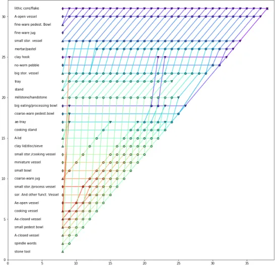
As an example, we will use an archeological data set from Alberti (2013). The original data set consists in a matrix whose lines are objects and columns some archeological site of the Punta Milazzese (Aeolian Archipelago, Italy) settlement. An element of the matrix is the number of time a given object (line) has been found in a given archeological site (column). The original dissimilarity is the L2 distance of the normalized data set: the smaller the dissimilarity between two objects, the more they are found together in a site. We applied Algorithm 6 on these data. We got the results depicted in Figure 1. The color are associated with a hierarchical decomposition of the hypergraph (Brucker and G´ely, 2009) and the cluster representation is an up
facing triangle if it has only one predecessor, a down facing triangle if it has only one successor (hence a losange if it is both) and a circle otherwise.
Figure 1: Clusters of the totally balanced approximation of the original L2 dissimilarity. Element order is a totally balanced one. Height is equal to the cardinal of the cluster
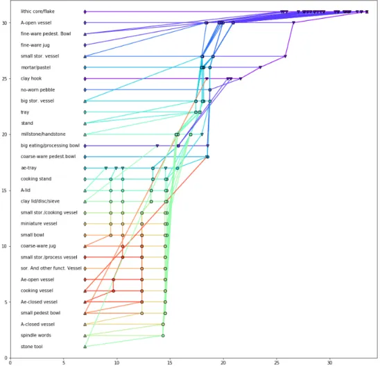
By drawing the clusters using the diameter as height (Figure 2), we see that a lot of clusters are really close: they are either on the same horizontal line (thus a truncated balls for the same origin. See for intance the horizontal line for the first element) and have very close diameter, or on the same ver-tical line and form a close cluster succession (see for instance the lower part
of Figure 2 and the 4 vertical cluster lines). Finally using totally balanced
Figure 2: Same as Figure 1 with height equal to the diameter of the cluster
structures allows us to:
• Find representatives of the clusters according to the center of the trun-cated balls of the clusters (graphically represented by the top edge ele-ment).
• Find an order between the elements.
• Organize the data along horizontal (succession for a same element) or vertical (cluster chain) lines.
7
Conclusion
We have shown in this paper that totally balanced structures can be used in clustering through a special kind of dissimilarities. These structures allow an efficient approximation scheme and a convenient graphical representation.
Finally, this work shows a new class of dissimilarities, chordal dissimilar-ities, which is a good model for classification as they admit only few clusters that can be easily computed and interpreted. We will further study these dis-similarities as they in order to determine more of their properties (structural bijections or graphical representations for instance).
8
References
Alberti G. (2013) Making Sense of Contingency Tables in Archaeol-ogy: the Aid of Correspondence Analysis to Intra-Site Activity Areas Research, Journal of Data Science, 11, 501-536.
Anstee R.P. (1983) Hypergraphs with no special cycles, Combinatorica, 3, 141-146.
Antsee R.P. and Farber M (1984), Characterizations of totally balanced matrices. Journal of Algorithms, 5, 215-230 (1984).
Bandelt, H.-J., Dress, A. W. M. (1989), “Weak Hierarchies Associated with Similarity Measures – an Additive Clustering Technique”, Bulletin of Mathematical Biology, 51, 133–166.
Barth´elemy and Brucker (2008), Binary Clustering. Journal of Discrete Applied Mathematics, 156, 1237-1250.
Bertrand, P. (2000), “Set Systems and Dissimilarities”, European Journal of Combinatorics, 21, 727 – 743.
Bertrand, P. and Diatta, J. (2014), Weak Hierarchies: A Central Cluster-ing Structure Clusters, Orders, And Trees: Methods and Applications, eds, F. Aleskerov, B. Goldengorin and P. M. Pardalo , Berlin: Springer-Verlag, chapter 14.
Brucker, F. (2005), From hypertrees to Arboreal Quasi-ultrametrics, Dis-crete Applied Mathematics, 147, 3–26.
Brucker, F. and G´ely, A. (2009), Parsimonious cluster systems, Advances in Data Analysis and Classification, 3, 189–204.
Brucker, F. and G´ely, A. (2010), Crown-free Lattices and Their Related Graphs” Order, 28:443–454.
Brucker, F. and Pr´ea. P. (2015), Totally Balanced Formal Concept Rep-resentations, Proceedings of ICFCA 215, 169-182.
Diatta, J., and Fichet, B. (1994), From Asprejan Hierarchies and Bandelt-Dress Weak-hierarchies to Quasi-hierarchies, New Approaches in Classi-fication and Data Analysis, Eds., E. Diday,Y. Lechevallier, M. Schader, P. Bertrand, and B. Burtschy, Berlin: Springer-Verlag, 111–118.
Dirac, G.A. (1961), On rigid circuit graphs, Abh. Math. Sem. Univ. Hamburg, 25 (1961) 71-76.
Farber, M. (1983), Characterizations of strongly chordal graphs, Discrete Mathematics, 43, 173-189.
Lehel, J. (1985), A Characterization of Totally Balanced Hypergraphs, Discrete Mathematics, 57, 59-65.
Lovasz L. (1968), Graphs and set systems, Beitr¨age zur Graphentheorie, Ed. H. Sachs et al. Teubner, Leipzig, 99-106.
Lubiw, A. (1987), Doubly lexical Orderings of Matrices, SIAM J. on Computing, 16, 854-879.
Spinrad, J. (1993), Doubly lexical Ordering of Dense 0-1 Matrices, In-formation Processing Letters, 45, 229-235.
Spinrad, J. (2003) Efficient Graph representations American Mathemat-ical Society, 2003.