UNIVERSITÉ DU QUÉBEC
VARIABLES ENVIRONNEMENTALES INFLUENÇANT LA DENSITÉ ET LA DIVERSITÉ DE LA MACROFAUNEÉPIBENTHIQUE ET LA BIOTURBATION
DANS L'ESTUAIRE ET LE GOLFE DU SAINT-LAURENT, CANADA
MÉMOIRE PRÉSENTÉ À
L'UNIVERSITÉ DU QUÉBEC À RIMOUSKI comme exigence partielle
du programme de maîtrise en océanographie
PAR
RÉNALD BELLEY
Service de la bibliothèque
Avertissement
La diffusion de ce mémoire ou de cette thèse se fait dans le respect des droits de son auteur, qui a signé le formulaire « Autorisation de reproduire et de diffuser un rapport, un mémoire ou une thèse ». En signant ce formulaire, l’auteur concède à l’Université du Québec à Rimouski une licence non exclusive d’utilisation et de publication de la totalité ou d’une partie importante de son travail de recherche pour des fins pédagogiques et non commerciales. Plus précisément, l’auteur autorise l’Université du Québec à Rimouski à reproduire, diffuser, prêter, distribuer ou vendre des copies de son travail de recherche à des fins non commerciales sur quelque support que ce soit, y compris l’Internet. Cette licence et cette autorisation n’entraînent pas une renonciation de la part de l’auteur à ses droits moraux ni à ses droits de propriété intellectuelle. Sauf entente contraire, l’auteur conserve la liberté de diffuser et de commercialiser ou non ce travail dont il possède un exemplaire.
11
RÉSUMÉ
L'estuaire et le golfe du Saint-Laurent (EGSL), Canada, subit présentement un évènement hypoxique qui pourrait être causé par des changements dans la composition de la masse d'eau de fond et une augmentation de l'apport en matière organique. Le fond marin de l'EGSL a été photographié à 11 stations durant les étés 2006 et 2007. Les images ont ensuite été analysées afin d'identifier les traces de bioturbation (Lebensspuren) et les organismes macrobenthiques présents.
Les objectifs de cette étude sont: 1) d'identifier les variables environnementales qui influencent la densité et la diversité de la macrofaune épibenthique ainsi que les traces de bioturbation, et 2) de déterminer les différences entre les régions de l'EGSL avec des niveaux d'oxygène élevés, moyens et bas.
La concentration d'oxygène dans la couche de fond est la variable environnementale qui explique le mieux les densités de traces totales et de surface : les densités de ces traces augmentent alors que l'oxygène diminue. La densité de traces plus élevée dans la région hypoxique de l'EGSL est principalement due au déposivore de surface Ophiura sp., qui se retrouve en grande densité dans cette région. Les résultats indiquent que les conditions hypoxiques actuelles n'affectent pas négativement la densité et la diversité des traces de bioturbation ainsi que la richesse spécifique. Cependant, nous avons observé dans la zone hypoxique une augmentation des déposivores de surface (tolérants aux basses concentrations d'oxygène) et une diminution des suspensivores (intolérants aux basses concentrations d'oxygène). Nous émettons l'hypothèse que la diminution de la concentration d'oxygène des eaux de fond au cours des dernières années a causé un changement dans la structure de la communauté macro-épibenthique de l'estuaire maritime du Saint-Laurent (EMSL). Les espèces avec une plus faible tolérance aux basses concentrations d'oxygène, qui sont généralement responsables des traces en relief, sont remplacées par des espèces plus tolérantes, tels que les déposivores de surface Ophiura sp., qui sont responsables de la majorité des traces de surface.
REMERCIEMENTS
Je tiens tout d'abord à remercier mon directeur Philippe Archambault, chercheur et professeur à l'Institut des sciences de la mer de Rimouski (ISMER), qui m'a épaulé tout au long de ma maîtrise. Philippe m'a permis d'étudier les fonds marins du Saint-Laurent, ce que je désirais ardemment. Il m'a conseillé, supporté dans les moments plus difficiles, permis de participer à des congrès internationaux et à un stage en France en plus de me guider durant toutes les étapes de ma maîtrise. Merci à mon co-directeur Bjorn Sundby, professeur à l'Institut des sciences de la mer de Rimouski (ISMER) et professeur adjoint à l'université McGill, pour ses conseils et son apport considérable tant au niveau scientifique que financier. Merci au Dr Franck Gilbert, chargé de recherche au CNRS, et à tous les membres de l'équipe du Laboratoire d'Écologie Fonctionnelle à Toulouse qui m'ont si bien accueilli dans leur laboratoire lors de mon stage et pour leurs discussions constructives sur la bioturbation. Merci au Dr Jean-Marc Gagnon, chef des collections de la division des invertébrés du Musée canadien de la nature, pour son aide considérable dans l'identification des organismes sur les photographies benthiques. Merci à Yvonnick Le Clainche, chercheur et professeur à l'Institut des sciences de la mer de Rimouski (ISMER), pour avoir accepté la présidence du jury de ce mémoire. Merci à Denis Gilbert, chercheur scientifique à l'Institut Maurice-Lamontagne, pour avoir accepté de faire partie du jury. Merci à toute l'équipe du laboratoire d'écologie benthique de Philippe, dont spécialement Mélanie Lévesque, Mylène Bourque, Annie Séguin, Laure de Montet y et Adeline Piot. Merci à tout l'équipage du
lV
Coriolis 1/ ainsi qu'aux chercheurs et étudiants qui m'ont aidé sur le bateau. Merci
à mes amis et collègues de l'ISMER qui ont apporté une contribution à ce projet scientifique. Un grand merci aux membres de ma famille qui ont toujours cru en moi et qui m'ont soutenu. Une mention spéciale à mon ami Simon Houle qui a su me changer les idées aux moments opportuns. Un grand merci de tout cœur à ma copine Sophie Roch qui m'a accompagné et soutenu tout au long de cette maîtrise. Merci à l'Université du Québec à Rimouski et au ministère de l'Éducation, du Loisir et du Sport du Québec de m'avoir donné une bourse pour de courts séjours d'études universitaires à l'extérieur du Québec (PBCSE) qui a servi à analyser des échantillons au Laboratoire d'Écologie Fonctionnelle. Merci au Conseil de recherches en sciences naturelles et en génie du Canada (CRSNG) et à Pêches et Océans Canada (MPO) pour avoir subventionné cette recherche.
TABLE DES MATIÈRES
RÉSUMÉ ... ii
REMERCIEMENTS ... iii
TABLE DES MATIÈRES ... v
LISTE DES TABLEAUX ... vii
LISTE DES FIGURES ... viii
LISTE DES ANNEXES ... x
INTRODUCTION GÉNÉRALE ... 1
CHAPITRE 1 : ENVIRONMENTAL VARIABLES INFLUENCING MACROBENTHIC AND BIOTURBATION DENSITY AND DIVERSITY IN THE ESTUARY AND GULF OF ST. LAWRENCE, CANADA ... 12
1.1 Introduction ... 13
1 .2 Materials and methods ... 17
1.2.1 Field sampling ... 17 1.2.2 Image analysis ... 18 1.2.3 Statistical analyses ... 20 1.3 Results ... 23 1.3.1 Univariate analyses ... 28 1.3.2 Multivariate analyses ... 35 1 .4 Discussion ... 40
VI
1.4.1 Macrobenthic epifauna ... 40
1.4.2 Bioturbation traces ... 43
1.4.3 The origins of bioturbation traces ... 47
1.4.4 Recent bioturbation ... 48
1.5 Conclusion ... 50
CONCLUSION GÉNÉRALE ... 52
RÉFÉRENCES ... 58
LISTE DES TABLEAUX
Table 1: List of suriace and relief-traces identified on benthic images from the
EGSL (based on Mauviel & Sibuet (1985) and Jones et al. (2007)), mean density
(area of seafloor covered by traces (%)) and overall density per station (%) ... 25
Table 2: Mean macrobenthic epifaunal density (ind. m-2) per taxa and per station
for the 11 stations sam pied in the Estuary and Gulf of St. Lawrence in 2006 and 2007 ... 26
Table 3: Summary of nested ANOVAs for total-traces density (log(x+1)),
suriace-traces density (log(x+1)), relief-traces density (loglO), grey-coloured sediment
density (...J...J) , total-traces diversity, suriace-traces diversity, relief-traces diversity,
species richness (S), Pielou's evenness (J) and Shannon-Wiener diversity (H) to
test the effect of oxygen level and station within oxygen level. ... 31
Table 4: Results of the multiple linear regression models (stepwise procedure) used to estimate total-traces density (%), suriace-traces density (%), relief-traces
density (%), grey-coloured sediment density (...J...J) (%), total-traces diversity
(loglO), suriace-traces diversity, relief-traces diversity, species richness, Pielou's
evenness (J) and Shannon-Wiener diversity (loge) (H) among the 11 stations
sam pied in the Estuary and Gulf of St. Lawrence in 2006-2007 ... 34
Table 5: Permutational analysis of variance (PERMANOVA) (Anderson, 2001;
McArdle & Anderson, 2001) results testing the effect of oxygen level and its
interaction with total-traces and organism densities based on Bray-Curtis similarity matrices periormed on untransformed and presence\absence transformed data ... 37
Table 6: Results of similarity percentage analyses (SIMPER) showing the
contribution (%) of the types of traces to the average Bray-Curtis dissimilarity of
compared oxy+, oxy- and hypoxic groups as weil as the average dissimilarity (%)
VlIl
LISTE DES FIGURES
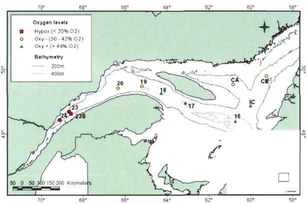
Figure 1: Stations sampled in the Estuary and Gulf of St. Lawrence, Canada, in August 2006 and July 2007. Oxy+ stations 16, 17, 18 and IC, and oxy- stations 19, 20, CA and CE were sampled in August 2006. The hypoxic stations 23, 23S and 24 were sampled in July 2007 ... 18 Figure 2: Representative photographs taken in the Estuary and Gulf of St. Lawrence in 2006 and 2007. A) Station 24: Ophiura sp. and detritus, B) Station 23: Ophiura sp., Actinauge sp. (right), Lycodes sp. (center right) in an
imprint-depression and close to a medium burrow, C) Station 20: Small burrows, medium
burrows with grey sediment (top right), double ploughs (from top left to down center), Pennatula aculeata (top center and down left) , Amphiura sp. arms (top left) and flatfish (top center) D) Station 19: Small and medium burrows, Pandalus
sp., Pennatula borealis, P. aculeata and Amphiura sp. arms, E) Station 18:
Small, medium and large burrows, imprints-depressions (top right), simple
ploughs (down right and down left), P. aculeata, P. borealis and unknown
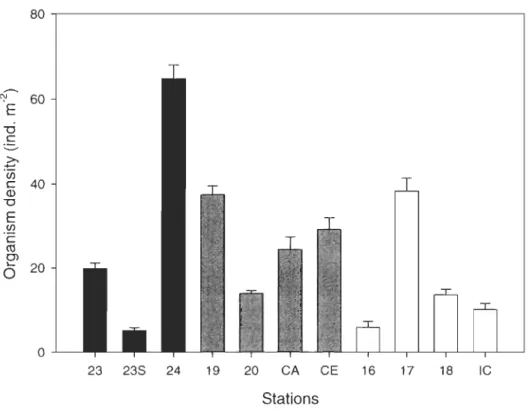
crustaceans, and F) Station IC: Sediment cloud (Ieft), shrimp trail (down center to top right), imprints-depressions and Pandalus sp ... 27 Figure 3: Mean total organism density (ind. m·2 ± SE) for the 11 stations sampled in the Estuary and Gulf of St. Lawrence in 2006 and 2007 ... 28
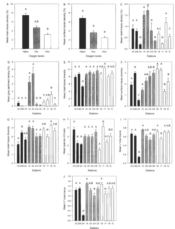
Figure 4: Mean (± SE) of: A) total-traces density (%) and B) surface-traces
density (%) for three different oxygen levels, and C) relief-traces density (%), D) grey-coloured sediment density (%), E) total-traces diversity, F) surface-traces diversity, G) relief-traces diversity, H) species richness, 1) Pielou's evenness (J') of total-traces and J) Shannon-Wiener's diversity index (H') of total-traces for stations within oxygen level. ... 32
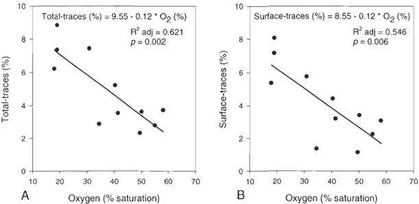
Figure 5: Relation between oxygen saturation (%) and A) total-traces density (%)
and B) surface-traces density (%) at the 11 stations sampled in the Estuary and
Gulf of St. Lawrence in 2006 and 2007 ... 35 Figure 6: Non-metric multi-dimensional scaling (nMDS) plots of total-traces density per oxygen level based on A) untransformed data and B) presence\absence transformed data ... 39
x LISTE DES ANNEXES
Annexe 1. Clé d'identification des traces de bioturbation (Lebensspuren)
Les océans recouvrent approximativement 70% de la surface terrestre,
constituant ainsi le plus grand écosystème qu'on y retrouve. En raison d'une utilisation toujours grandissante de cet écosystème par l'Homme, plusieurs habitats marins subissent des pressions anthropogéniques importantes telles que la pêche, la pollution, le développement côtier et le réchauffement climatique. Prises individuellement ou agissant en synergie, ces pressions peuvent mener à une perte de biodiversité marine (Snelgrove, 1998; Snelgrove et aL, 2000; Worm et aL, 2006). Cette biodiversité marine est composée en majeure partie d'organismes benthiques habitant sur (épifaune) et dans
(endofaune) les sédiments (Snelgrove, 1999). Plusieurs études ont démontré les effets importants qu'ont les organismes benthiques sur les sédiments marins tels que les processus biochimiques (Aller et aL, 2001; Meysman et aL, 2006;
Middelburg & Levin, 2009), la géomorphologie (Murray et aL, 2002), et la production primaire et secondaire (Snelgrove, 1998). La perte de biodiversité benthique marine aurait potentiellement des effets néfastes importants sur les fonctions et la santé des écosystèmes, ainsi que sur les processus marins (Snelgrove, 1998; Worm et aL, 2006).
2
Influence des variables environnementales sur les communautés benthiques
Les communautés benthiques sont aussi affectées par différentes variables environnementales de leur milieu. Les caractéristiques du substrat telles que la taille des sédiments (Warwick et aL, 1991; Kostylev et aL, 2001) et la teneur en matière organique (Pearson & Rosenberg, 1978; Rosenberg, 1995) sont reconnues comme étant des variables qui influencent la distribution et la structure des communautés benthiques. D'autres variables environnementales telles que la profondeur et la vitesse du courant (Kostylev et aL, 2001), ainsi que la température et la salinité (Pearson & Rosenberg, 1978) sont aussi reconnues pour avoir un impact important sur la distribution et la structure des communautés benthiques. Cependant, parmi toutes les variables environnementales affectant les habitats marins, Diaz & Rosenberg (2008) rapportent que l'oxygène dissous est celle qui a changé le plus drastiquement depuis les années 1960. La diminution de l'oxygène dissous est un facteur bien étudié ayant des conséquences nuisibles pour les environnements marins. Cette diminution de l'oxygène dissous est très souvent due à une eutrophisation de nature anthropogénique, soit un apport accru de nutriments dans les eaux. Depuis les années 1960, les zones dépourvues de ressources de pêches en raison d'évènements hypoxiques dans les océans côtiers, appelées zones mortes, se sont propagées de façon exponentielle: aujourd'hui, des zones mortes sont répertoriées dans plus de 400 systèmes et couvrent une superficie
de plus de 245 000 km2 (Diaz & Rosenberg, 2008). La diminution de l'oxygène dissous sous la valeur hypoxique généralement acceptée de 62,5 Ilmol L-1 ou 2 mg L-1 (Gilbert et al., 2005), cause une réduction de la croissance, de
l'alimentation et de la valeur d'adaptation (ou « fitness » individuel) des animaux marins (Wu, 2002). Cependant, Vaquer-Sunyer & Duarte (2008) ont démontré que les organismes benthiques ont des seuils de tolérance variables à l'hypoxie et qu'une concentration de 2 mg L-1 peut être létale pour plusieurs espèces. Néanmoins, l'hypoxie est reconnue pour forcer les organismes endobenthiques
à
migrer vers la surface des sédiments et, en conséquence, ces organismes deviennent plus vulnérables à la prédation (Llans6, 1992; Wu, 2002). En éliminant certaines espèces sensibles, l'hypoxie est aussi reconnue pour affecter la fonction et la structure des communautés en réduisant la diversité et la richesse spécifique (Diaz & Rosenberg, 1995; Wu, 2002). De plus, certaines études font mention que les suspensivores peuvent être remplacés par les déposivores dans des conditions hypoxiques (Diaz & Rosenberg, 1995; Wu,2002).
Le Saint-Laurent et le phénomène hypoxique
Cette étude a été réalisée dans l'estuaire et le golfe du Saint-Laurent (EGSL), Canada. La présence du Chenal Laurentien, long de 1240 km et d'une profondeur variant entre 300 et 500 m, domine la morphologie de l'estuaire et du golfe du Saint-Laurent. La colonne d'eau du Chenal est stratifiée et est
4
composée de trois couches d'eau (Bugden, 1991). La couche de surface,
d'environ 50 m, démontre de grandes variations de température et de salinité en réponse aux changements de flux de chaleur saisonniers et aux débits d'eau douce. La couche intermédiaire froide, qui s'étend de 50 à 150 m, démontre quant à elle de plus faibles variations saisonnières que la couche de surface. Il est reconnu que la couche de surface se fusionne avec la couche intermédiaire froide en hiver. La couche profonde, plus chaude, s'étend jusqu'au fond et subit des changements à long terme (Bugden, 1991). Cette couche profonde est formée du mélange, en proportion variable, d'eau froide bien oxygénée provenant du courant du Labrador ainsi que d'eau chaude moins oxygénée de la partie centrale de l'Atlantique nord transportée par le Gulf Stream. Le mélange de ces masses d'eau s'engage dans le Chenal Laurentien par son embouchure situé au rebord du plateau continental et se dirige lentement vers la tête des trois chenaux, un voyage de quelques années (Gilbert et aL, 2005, 2007).
La concentration d'oxygène dans la couche profonde a diminué drastiquement depuis 1932 (Gilbert et aL, 2005, 2007). Dans cette couche d'eau de l'estuaire maritime du Saint-Laurent (EMSL), Gilbert et al. (2005, 2007) ont découvert que la concentration d'oxygène dissous a diminué de près de 50% pour la période couvrant 1932 à 2003, passant de 125 Ilmol L-1 de moyenne à 65 Ilmol L-1. En juillet 2003, environ 110 km de fond marin de la section longitudinale du Chenal Laurentien, situé dans l'EMSL, baignaient dans des eaux hypoxiques sous 60 Ilmol L-1.
À
cette même période, une concentration aussibasse que 51,2 J.1mol L-1 (16,2% de saturation) a été enregistrée
à
la station 23S (Fig. 1). De plus, la partie en amont du Chenal Laurentien, une aire couvrant 1300 km2, était hypoxique en permanence avec des concentrations d'oxygène sous 62,5 J.1mol L-1 ou 2 mg L-1 (Gilbert et aL, 2005, 2007). Cette diminution d'oxygène serait principalement due à deux facteurs. Premièrement, une augmentation de 1 ,65°C de la température de la couche d'eau de fond pour la période de 1932 à 2003 suggère un changement de la proportion du mélange des masses d'eau formant la couche d'eau de fond du Chenal Laurentien. Ce changement contribuerait d'une demie à deux tiers de la diminution en oxygène. Deuxièmement, une augmentation de la demande en oxygène des eaux profondes et du sédiment due à une augmentation de l'apport en matière organique serait responsable de la partie restante de la diminution en oxygène (Gilbert et aL, 2005; Thibodeau et aL, 2006; Katsev et aL, 2007). En effet, Thibodeau et al. (2006) rapportent une augmentation de la productivité marine dans l'EMSL depuis les années 1960. Cette augmentation de la productivité marine est reflétée par une augmentation du taux d'accumulation des kystes de dinoflagellés et des foraminifères benthiques. De plus, ils ont observé l'apparition de deux espèces de foraminifères benthiques tolérantsà
de basses concentrations d'oxygène et à des flux élevés de matière organique depuis les 40 dernières années.Des études ont démontré que l'hypoxie (Diaz & Rosenberg, 1995; Ritter & Montagna, 1999) et l'enrichissement en matière organique (Pearson &
6
Rosenberg, 1978) peuvent mener à une diminution de la biomasse, de l'abondance et de la biodiversité. Ces deux facteurs pourraient ainsi avoir des effets néfastes sur la densité et la diversité des organismes benthiques ainsi que sur la bioturbation des sédiments de l'EGSL.
La bioturbation
Au sens large, le terme bioturbation peut être défini comme étant le mélange et le transport de terre ou de particules de sédiment par différents organismes, incluant les microbes, les racines des plantes et les animaux fouisseurs (Rhoads, 1974; Meysman et aL, 2006). L'importance de la bioturbation a été comprise en premier lieu par Charles Darwin, qui lui a dédié son dernier livre scientifique (Darwin, 1881). La bioturbation faite par les organismes fouisseurs, aussi appelés « ingénieurs de l'écosystème », a eu et continue d'avoir un rôle crucial à jouer dans l'évolution de la vie sur terre (Meysman et aL, 2006). Ses organismes fournissent divers services clés aux écosystèmes. Ils sont en effet directement impliqués dans les cycles biogéochimiques du carbone et des nutriments (Solan et aL, 2008), dont plus spécifiquement le processus de minéralisation de la matière organique à
l'interface eau-sédiment (Gilbert et aL, 2003; Maire et aL, 2008). De plus, à travers leurs diverses activités, ils modifient les propriétés physiques (ex: le transport sédimentaire) et biologiques (ex: réseau trophique pélagique) du sédiment (Maire et aL, 2008; Van Colen et aL, 2008). La perte de telles espèces
ingénieures pourrait avoir des impacts négatifs importants sur la biodiversité et
les processus biochimiques à l'interface eau-sédiment (Coleman & Williams,
2002; Lohrer et aL, 2004; Solan et aL, 2004a).
Les traces de bioturbation sont aussi connues sous le nom de Lebensspuren, un mot allemand signifiant «trace de vie ». Elles peuvent être séparées en deux groupes principaux selon leur morphologie: les traces de surface et les traces en relief (Mauviel & Sibuet, 1985). Les traces de surface sont formées lorsque les organismes remanient uniquement les premiers centimètres du sédiment (ex: pistes, rides, sillons, etc.). Ces traces impliquent un mélange du sédiment qui peut être important en surface, mais qui n'affecte pas les particules situées profondément dans la colonne de sédiment. Quant aux traces en relief, elles sont formées lorsque les organismes mélangent le sédiment plus en profondeur lors de la formation ou de la maintenance de leurs diverses structures (ex: terriers en forme de fente, terriers simples, tumulus crevassés, etc.). Ce type de bioturbation, aussi appelé bioirrigation, implique le transport de l'eau interstitielle par des organismes benthiques lors de diverses activités telles que l'alimentation, l'enfouissement, la locomotion et la ventilation du terrier (Maire et aL, 2008). Pour cette raison, il est présumé être plus important pour l'oxygénation et les processus biochimiques à l'intérieur de la colonne de sédiment « perforée».
8
La photographie benthique
Au cours des dernières décennies, la prise de photographies benthiques a prouvé son efficacité à identifier les organismes benthiques ainsi qu'à caractériser et à quantifier les traces de bioturbation (Heezen & Hollister, 1971; Kitchell, 1979; Mauviel & Sibuet, 1985; Solan et aL, 2003; Jones et aL, 2007). En particulier, cette technique est reconnue comme étant plus rapide que d'autres techniques d'échantillonnage benthique (benne, carottier, chalut, etc.) et a l'avantage de peu perturber l'environnement échantillonné (Kostylev et aL, 2001). Cependant, les études des traces de bioturbation et de la macrofaune épibenthique qui y est associée, ayant été menées avec la technique de photographie benthique, ont principalement été réalisées pour décrire des environnements néritiques à moins de 200 m et des environnements abyssaux situés à plus de 2000 m de profondeur. En contrepartie, à notre connaissance aucune étude sur le même sujet dans des environnements bathyaux (entre 200 et 2000 m), tel que le Chenal Laurentien, n'a été publiée. Par contre, dans l'EMSL, Hutin et al. (2005) ont mené une étude en utilisant la photographie benthique afin de déterminer le lien entre le signal acoustique d'un sonar multi-faisceaux et un banc de pétoncle d'Islande (Chlamys islandica). Toutefois, aucune étude portant sur les traces de bioturbation faites à la surface du sédiment de l'EGSL n'a été publiée jusqu'à maintenant. Une étude menée à bord du submersible Pisces IV (Syvitski et aL, 1983) a permis de recueillir des données sur le benthos de la zone bathyale du Chenal Laurentien. Cependant,
mis
à
part la mention de la présence plus ou moins importante des traces de bioturbation, aucune donnée quantitative n'a été fournie.Communautés benthiques du Saint-Laurent
Les organismes benthiques du Chenal Laurentien sont encore peu connus. Les études pionnières de Préfontaine & Brunei (1962) et de Peer (1963) sur les organismes endobenthiques ont pavé la voie aux études de Robert
(1979) sur les mollusques, de Massad (1975) et de Massad & Brunei (1979) sur
les polychètes ainsi que de Ouellet (1982) sur la macrofaune endobenthique de l'EMSL. Récemment, des études ont été menées dans l'EGSL sur les relations entre les variables environnementales et la faune endobenthique (Desrosiers et al., 2000; Bourque, 2009) ainsi que la faune épibenthique (Lévesque et al., 2008; Lévesque, 2009).
En règle générale, il est reconnu que l'abondance et la diversité des espèces dans un estuaire diminuent de l'océan vers l'amont (Rapoport, 1994; Schaffner et al., 2001). Pour ce qui est de l'EGSL, l'étude de Bourque (2009) a également permis de démontrer que la structure des communautés endobenthiques est spécialement affectée par la diminution de l'oxygène. En effet, elle observe une réduction de la richesse spécifique et de la diversité de Shannon pour la période couvrant 1980
à
2005-2006. Elle observe aussi une augmentation des espèces opportunistes à la surface des sédiments, telles que10
Myriochele sp., qui sont généralement présentes dans les environnements perturbés par l'hypoxie. Les études de Lévesque et al. (2008) et de Lévesque
(2009) ont quant à elles démontré l'importance de l'oxygène dissous comme variable environnementale structurant les communautés épibenthiques de l'EGSL. En effet, ces études rapportent une plus grande densité de cnidaires et de mollusques (tolérants aux basses concentrations d'oxygène) et une moins grande densité de crustacés (intolérants aux basses concentrations d'oxygène) dans la zone hypoxique que partout ailleurs dans l'EGSL. En plus des connaissances que nous avons des communautés benthiques en général, ces études démontrent l'importance de l'oxygène dissous comme variable environnementale structurant les communautés benthiques de l'EGSL.
Objectifs et hypothèses
Les objectifs de cette étude étaient de: 1) déterminer les variables environnementales qui influencent la densité et la diversité macrobenthiques ainsi que les traces de bioturbation, et 2) déterminer s'il y a une différence significative entre les régions du fond marin de l'EGSL avec des concentrations d'oxygène faibles, moyennes et élevées. Les hypothèses étaient que : 1) la concentration en oxygène dissous sera la variable environnementale qui influencera le plus la densité et la diversité macrobenthique ainsi que les traces de bioturbation, et 2) la région hypoxique de l'EGSL aura une richesse spécifique
plus basse que les régions normoxiques, ce qui engendrera une plus faible densité et diversité des traces de bioturbation.
Ce mémoire de maîtrise, sous forme d'article scientifique, est rédigé en anglais et contient un chapitre. Cet article sera soumis à la revue Aquatic Bi%gy
CHAPITRE 1
ENVIRONMENTAL VARIABLES INFLUENCING
MACROBENTHIC AND BIOTURBATION DENSITY
AND DIVERSITY IN THE ESTUARY AND GULF OF
1.1 Introduction
Many marine habitats are presently under pressure by multiple anthropogenic threats su ch as fishing, pollution, coastal development, and global warming. Any one of these threats can lead to a loss of marine biodiversity (Snelgrove, 1998; Worm et aL, 2006). Marine benthic organisms have important effects on sedimentary biogeochemical processes (Aller et aL, 2001; Meysman et aL, 2006; Middelburg & Levin, 2009), geomorphology (Murray et aL, 2002), and primary and secondary productivity (Snelgrove, 1998). The loss of marine macrobenthic biodiversity would likely have negative effects on ecosystem functions, processes and health (Snelgrove, 1998; Worm et aL, 2006).
Benthic communities are also affected by different environ mental variables. Characteristics of the substratum such as the sediment grain size (Kostylev et aL, 2001) and the organic matter content (Pearson & Rosenberg, 1978; Rosenberg, 1995) are known to influence benthic community distribution and structure. The decrease of dissolved oxygen, more often due to anthropogenic eutrophication, is a well-known deleterious factor for marine environments (Diaz & Rosenberg, 2008). The decrease of dissolved oxygen below the generally accepted hypoxic value of 62.5 Ilmol L-1 or 2 mg L-1 (Gilbert et aL, 2005) is known to reduce growth, feeding and individual fitness of marine animais (Wu, 2002). However, Vaquer-Sunyer & Duarte (2008) demonstrated that marine benthic organisms have varying thresholds to hypoxia and that a
14
concentration of dissolved oxygen of 2 mg L-1 is lethal for many species. Nonetheless, hypoxia is known to force infaunal organisms to move doser to the sediment surface and, in consequence, become more vulnerable to predation (Llans6, 1992; Wu, 2002). Sy eliminating sensitive species, hypoxia is also known to affect community structure and function by reducing species diversity and species richness (Diaz & Rosenberg, 1995; Wu, 2002). Moreover, it is reported that under hypoxic conditions suspension feeders can be replaced by deposit feeders (Diaz & Rosenberg, 1995; Wu, 2002).
The present study was carried out in the Estuary and Gulf of St. Lawrence (EGSL), Canada. This environ ment is dominated by the 1240 km long, 300 to 500 m deep, Laurentian Channel. The water column in the Channel is stratified,
with a surface layer (upper 50 m), a cold intermediate layer (50 to 150 m) and a deep warmer layer (below 150 m) (Sugden, 1991). In the Lower St. Lawrence estuary (LSLE), Gilbert et al. (2005) found that the oxygen concentration in the deep layer of water decreased by 50%, from 125 Ilmol L-1 to 65 Ilmol L-1, for the 1932-2003 period. In July 2003, the landward region of the Laurentian Channel,
an area covering 1300 km2, was hypoxic with concentrations of dissolved oxygen lower th an 62.5 Ilmol L-1 (Gilbert et aL, 2005). An increase in organic carbon loading and changes in water mass composition are the principal causes (Gilbert et aL, 2005; Thibodeau et aL, 2006; Katsev et aL, 2007). Hypoxia (Diaz & Rosenberg, 1995; Ritter & Montagna, 1999) and organic enrichment (Pearson &
Rosenberg, 1978) can lead to decreasing biomass, abundance and biodiversity,
with possible negative effects on sediment bioturbation.
Bioturbation can be broadly defined as the mixing and transport of particles and solutes within sediments and soil by various organisms, including microbes, rooting plants and burrowing animais (Rhoads, 1974; Meysman et aL,
2006). Bioturbation created by burrowing organisms, sometimes called
"ecosystem engineers", had and still has a crucial role in the evolution of life on earth (Meysman et aL, 2006). The loss of engineer species could have important negative effects on biodiversity and on biogeochemical processes at the water-sediment interface (Coleman & Williams, 2002; Lohrer et aL, 2004; Solan et aL,
2004a; Middelburg & Levin, 2009).
Bioturbation traces are also known as "Lebensspuren", a German term meaning life traces. They can be separated in two main groups, surface-traces and relief-traces, according to their morphology (Mauviel & Sibuet, 1985). Surface-traces are formed when organisms rework only the first few centimetres of the sediment, which leaves traces in the form of ploughs, tracks, furrows, etc. These traces imply sediment mixing that can be important, but which does not affect particles located deep within the sediment. In contrast, relief-traces, in the shape of simple burrows, slit-shaped burrows, crevassed mounds, etc., are formed when organisms rework sediments to much greater depths. This kind of
16 bioturbation is thought to be more important for oxygenation and biogeochemical processes deeper within the "perforated" sediment.
Over the last decades, benthic photography has proven its reliability to identify organisms and to characterise and quantify bioturbation traces (Heezen
& Hollister, 1971; Kitchell, 1979; Mauviel & Sibuet, 1985; Solan et al., 2003;
Jones et al., 2007). In particular, the photographie technique is known to be less time consuming th an other benthic sampling techniques (grab, box-core, trawl,
etc.) and has the advantage of leaving the environment mostly undisturbed (Kostylev et al., 2001).
The objectives of this study were to determine the environmental variables influencing the density and diversity of macrobenthic epifauna and bioturbation traces, and to determine if there are significant differences among regions of the seafloor in the ESGL with high, medium and low oxygen levels. This was accomplished using benthic photography and different environ mental measurements. The hypotheses are that 1) the oxygen concentration will be the most important environmental variable influencing the density and diversity of macrobenthic epifauna and bioturbation traces, and 2) the hypoxic region of the EGSL will have lower species richness and consequently, lower bioturbation trace density and diversity th an normoxic regions.
1.2 Materials and methods
1.2.1 Field sampling
The study was conducted in the Estuary and Gulf of St. Lawrence (EGSL) on board the RV Coriolis Il in August 2006 and July 2007 (Fig. 1). Eight stations were samples from August 8th to 21 st 2006 and three from July
i
h to 9th 2007. Thirty images were taken at each of the 11 stations. The photographs were taken with a bottom contact Benthos underwater camera system equipped with a Pentax Optio MX4 digital camera of a resolution of 4.0 Megapixels mounted perpendicular to the seafloor. The mean (± SE) area covered by each image was 0.82 ± 0.02 m2.At each station, the deep layer water temperature and salinity were recorded with a Seabird CTD. Water samples were collected from the deep layer using 12 L Niskin® bottles (General Oceanics®) to corroborate CTD values and measure oxygen concentration. Dissolved oxygen was determined by Winkler titration (Grasshoff et aL, 1999).
Surface layer sediments were collected from the top 5 cm of a boxcore or a Van Veen grab sample, and granulometric characteristics were analysed using a LS 13320 Beckman-Coulter Particle Size Analyser (Blott et aL, 2004). Also, the
18
total organic content in the sediments was determined by the loss-on-ignition method (Dean, 1974). 64° Oxygen levels
•
Hypox « 20% 02) 0 Oxy -(30 -42% 02)•
Oxy + (> 49% 02) Bathymetry .'ta..-. . ° 200m 0 1[) _ .. _,-'" 400mC
50D
70° 68° 66° 64° 62° 60° 58°Figure 1: Stations sampled in the Estuary and Gulf of St. Lawrence, Canada, in August 2006 and July 2007. Oxy+ stations 16, 17, 18 and IC, and oxy- stations 19, 20, CA and CE were sampled in August 2006. The hypoxic stations 23, 23S and 24 were sampled in July 2007.
1.2.2 Image analysis
To determine the number of images to be analysed, we used the data from stations 20, 23 and IC to plot 1) a species and traces accumulation curve and 2) the mean and the variance of the accumulated species and traces. Both techniques lead to the conclusion that the analysis of fifteen images would give a
good estimate of the species and traces at a given station. Fifteen images were then randomly chosen for each station, except for station CA, where only 7 images were usable. A total of 157 images were analysed using the image analysis software "lmageJ" (http://rsb.info.nih.gov/ij/index.html). On each image, macrobenthic epifaunal organisms were identified to the lowest taxonomie level possible and counted. Identification was also confirmed with organisms collected with a Van Veen grab and an USNEL box core for a project on the infauna (Bourque, 2009). The abundances were converted to number per m2. Since only the arms of the Ophiuridae Amphiura sp. were visible, the total number of arms counted on a single image was divided by five to give the number of individuals. We recognize that this procedure could underestimate the number of individuals since not ail five arms of each individual will always be extended to the sediment surface (Rosenberg, 1995). The area of each trace was manually encircled to determine the density of traces on each image. The area covered by surface-traces was measured and the number and the area of the relief-surface-traces were determined. Due to the limited resolution of the images, only organisms and bioturbation traces ~ 5 mm were identified.
Images were first examined to determine the types of bioturbation traces present. Based on the classification of Mauviel & Sibuet (1985) and Jones et al. (2007), an identification key was produced to represent the different traces found on the images (Appendix 1). These traces were classified based on their morphology. They were separated into two groups, surface-traces and
relief-20
traces, which were then separated into distinctive traces. The area covered by
the different types of traces was determined and is hereafter referred as "trace
density". The area of small burrows was determined by approximating the burrow
opening as a circle (A=TT·f). A median burrow radius of 0.0075 m was used to calculate a median burrow area, which was th en multiplied by the number of small burrows on the image to obtain an estimate of the total area of burrows
openings. The area occupied by sm ail slit-shaped burrows was determined by
approximating their shape as a rectangle (Area=Width·Height) of median width 0.002 m and median length 0.0075 m. The total area occupied at the sediment
surface by small slit-shaped burrows was then estimated from their number on
an image. The area of seafloor occupied by macrobenthic epifauna was included
in the total-traces density, surface-traces density and relief-traces density since
organisms were presumably forming traces at the time the image was taken. The
area of seafloor occupied by Ophiura sp., Ctenodiscus crispa tus, Panda/us sp.,
Sebastes sp. and Rajidae was added to the surface-traces density while the area of the basal disc of Cnidarians was added to the relief-traces density.
1.2.3 Statistical analyses
Univariate indices of bioturbation traces and macrobenthic epifaunal diversity were calculated for each image. Univariate indices of bioturbation traces
are: traces density (%), traces diversity (total number of different types of traces),
univariate index of macrobenthic epifaunal diversity was species richness (S) and corresponds to the number of species counted.
Stations were pooled based on their oxygen concentration. Groups were composed of stations with: i) > 49% O2 saturation (oxy+: stations 16, 17, 18 and IC), ii) between 30 and 42% O2 saturation (oxy-: stations 19, 20, CA and CE), and iii) < 20% O2 saturation (hypoxic: stations 23, 23S and 24).
Nested analyses of variance (ANOVA) were performed to determine if there was a significant difference between the oxygen levels (> 49% O2 , 30-42%
O2 and < 20% O2) and the stations within these oxygen levels. This was followed by post-hoc Tukey tests for multiple comparisons when significant differences were observed. Normality of residuals was verified with the Shapiro-Wilk test and their homogeneity was verified visually (Quinn & Keough, 2002). Variables that did not satisfy these criteria were transformed (fourth root (""), 10glO or IOg(X+1)
when data contained zero values) and are indicated in the tables.
Multiple linear regressions were also performed using the stepwise procedure (probability to enter of 0.25 and 0.10 to leave) to determine environmental factors influencing traces density, traces diversity, species richness (S), Shannon-Wiener diversity index (H) and Pielou's evenness index (J). The VIF (variance inflation factor) multicollinearity test was performed to
22
select environ mental factors with value lower th an 10, a threshold indicating a strong collinearity between variables (Quinn & Keough, 2002). The six environmental factors retained were depth (0), mean sediment grain size (MGS),
percent oxygen saturation (02), percent total organic matter (TOM), temperature (T) and salinity (S). Dependent variables used were total-traces density (%),
surface-traces density (%), relief-traces density (%), grey-coloured sediment density (%), total-traces diversity, surface-traces diversity, relief-traces diversity,
species richness (S), Shannon-Wiener diversity (Hj and Pielou's evenness (Jj. Adjusted ~ was the criterion used to determine the environmental variables best explaining the indices. The normality was verified on residuals with the Shapiro-Wilk test and their homogeneity was verified visuallY (Quinn & Keough, 2002).
Variables that did not satisfy these criteria were transformed ("" or 10glO)'
Multivariate analyses were based on Bray-Curtis similarity matrices performed on untransformed and transformed presence\absence data. Taxa that appeared only once were excluded from these analyses (Clarke & Warwick,
1994). Variations in traces densities and macrobenthic epifaunal densities were studied using a permutational multivariate analysis of variance (PERMANOVA) performed with 4999 random permutations of appropriate units (Anderson, 2001; McArdle & Anderson, 2001). When there were too few possible permutations to obtain a reasonable test, a p-value was calculated using 4999 Monte Carlo random draws from the asymptotic permutation distribution (Terlizzi et al., 2005). Significant terms within the full models were analysed using appropriate pair-wise
comparisons. Non-metric multidimensional scaling (nMDS) ordinations of similarity matrices were performed to visualize multivariate patterns. Similarity percentage analyses (SIMPER) were used to determine bioturbation traces that contributed the most to the dissimilarity between oxygen levels (Clarke, 1993).
1.3 Results
Eighteen types of surface-traces and nine types of relief-traces were identified (Table 1). A total of 2654 organisms were identified, representing 22 different macrobenthic taxa (Table 2). Some representative images of organisms and traces found in the EGSL are presented in Fig. 2. The organisms with the highest density were two brittlestars Ophiura sp., followed by Amphiura sp. Other organisms found in high densities were the anemones Edwardsia sp. and the stalked tunicate Boltenia ovifera (Table 2).
ln general, surface-traces covered a greater seafloor area than relief-traces, with the exception of stations 18 and 19 (Table 1). Imprints-depressions were the only type of surface-traces found at ail stations in the EGSL. Simple ploughs were found at ail stations except station 24. The Ophiura trace was the surface-trace with the highest density for a single station; this trace covered 7% of the seafloor at station 24. This trace was only found at the hypoxic stations 23
24
and 24. Shrimp trails were found at each oxy+ and oxy- stations where, except at station 16, Panda/us sp. was also recorded (Table 2).
Small burrows were found at ail stations (Table 1). They were the most abundant relief-trace in numbers. Although they covered a small area of the seafloor, they were the relief-trace with the highest density except at station CA where large burrows had the highest density. Medium burrows and medium slit-shaped burrows were also found at ail stations. Large burrows were found at ail stations except at stations 17 and CE. Although sm ail slit-shaped burrows were the second most abundant relief-trace in number, their density was low.
The highest density of organisms was found at the hypoxic station 24 (64.84 ind. m-2), which was dominated by Ophiura sp. (61.32 ind. m-2; Fig. 3 and Table 2). The lowest densities of organisms were found at the hypoxic station 23S and the oxy+ station 16 (5.14 ind. m-2 and 5.87 ind. m-2 respectively; Fig. 3 and Table 2). Panda/us sp. and unknown crustaceans were only found at oxy+ and oxy- stations, as was the case for B. ovifera and unknown bryozoans. Actinauge sp. and Cerianthus sp. were only found at hypoxic stations.
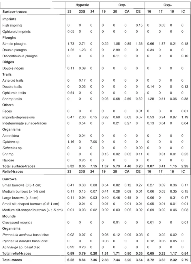
Table 1: List of surface and relief-traces identified on benthic images fram the EGSL (based on Mauviel & Sibuet (1985) and Jones et al. (2007)), mean density (area of seafloor covered by traces (%)) and overall density per station (%).
Hypoxic Oxy- Oxy+
Surface-traces 23 235 24 19 20 CA CE 16 17 18 IC
Imprints
Fish imprints 0 0 0 0 0 0 0.15 0 0.03 0 0
Ophiuroid imprints 0.05 0 0 0 0 0 0 0 0 0 0
Ploughs Simple ploughs 1.73 2.71 0 0.22 1.05 0.89 1.33 0.66 1.87 0.21 0.18 Double ploughs 1.25 1.23 0 0 2.99 0 0 0.34 0 0 0 Discontinuous ploughs 0 0 0 0 0.11 0 0 0 0 0 0.10 Ridges Double ridges 0.11 0.39 0 0 0 0 0 0 0 0 0 Trails Asteroid trails 0 0.17 0 0 0 0 0 0 0 0 0 Double trails 0 0.03 0 0 0 0 0 0.14 0 0 0.13 Ophiuroid trails 0.54 0 0 0 0 0 0 0 0 0 0 Shrimp trails 0 0 0 0.08 0.68 2.59 0.82 1.28 0.51 0.06 0.38 Others Feces 0 0 0 0 0 0 0.01 0 0 0 0.01 Imprints-depressions 0.47 2.00 0.15 0.92 0.68 0.63 0.67 0.53 0.94 0.87 1.19 Indeterminate surface-traces 0 0.54 0 0 0.21 0.27 0 0.13 0.04 0 0.04 Organisms Asteroidea 0 0.04 0 0 0 0 0 0 0 0 0 Ophiura sp. 1.16 0 7.00 0 0 0 0 0 0 0 0 Sebastes sp. 0 0 0 0 0 0 0.09 0 0 0 0 Shrimp 0 0 0 0.15 0.02 0.02 0.11 0 0.01 0.01 0.23 Rajidae 0 0.95 0 0 0 0 0 0 0 0 0
Total surface-traces 5.32 8.05 7.15 1.37 5.73 4.40 3.20 3.07 3.41 1.15 2.25
Relief-traces 23 235 24 19 20 CA CE 16 17 18 IC
Burrows
Small burrows (0.5-1 cm) 0.41 0.30 0.08 0.54 0.82 0.12 0.27 0.27 0.09 0.36 0.17 Medium burrows (> 1-5 cm) 0.11 0.15 0.07 0.41 0.28 0.09 0.01 0.06 0.03 0.35 0.15 Large burrows (> 5 cm) 0.11 0.04 0.03 0.40 0.46 0.45 0 0.06 0 0.31 0.17 Small slit-shaped burrows (0.5-1 cm) 0 0.01 0 0.01 0 0.01 0.01 0.05 0.01 0.01 0.01 Medium slit-shaped burrows (> 1-5 cm) 0.01 0.03 0.02 0.02 . 0.03 0.05 0.02 0.09 0.02 0.06 0.03 Mounds
Crevassed mounds 0 0 0 0 0.01 0 0 0.01 0 0 0.01
Organisms
Pennatula aculeata basal disc 0.02 0.07 0 0.05 0.12 0.09 0.03 0 0.02 0.02 0
Pennatula borealis basal disc 0 0 0 0.08 0 0 0 0.12 0.06 0.05 0
Actinauge sp. basal disc 0.22 0.20 0 0 0 0 0 0 0 0 0
Total relief-traces 0.89 0.79 0.20 1.51 1.71 0.80 0.35 0.65 0.23 1.17 0.54 Total-traces 6.22 8.84 7.36 2.88 7.44 5.20 3.54 3.72 3.63 2.32 2.79
26
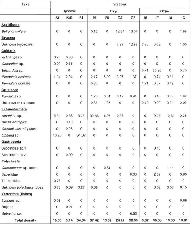
Table 2: Mean macrobenthic epifaunal density (ind. m-2) per taxa and per station
for the 11 stations sampled in the Estuary and Gulf of St. Lawrence in 2006 and
2007.
Taxa Stations
Hypoxic Oxy- Oxy+
23 23S 24 19 20 CA CE 16 17 18 IC Ascidiacea Bo/tenia ovifera 0 0 0 0.12 0 12.54 13.07 0 0 0 1.99 Bryozoa Unknown bryozoans 0 0 0 0 0 7.29 12.98 3.85 6.62 0 1.00 Cnidaria Actinauge sp. 0.95 0.86 0 0 0 0 0 0 0 0 0 Cerianthus sp. 0.09 0.11 0 0 0 0 0 0 0 0 0 Edwardsia sp. 0 0 0 0 0 0 0 0.71 26.90 0 0.70
Pennatula aculeata 1.04 2.94 0 2.17 5.00 3.97 1.37 0 0.74 0.81 0
Pennatula borea/is 0 0 0 0.83 0 0 0 1.21 0.57 0.49 0 Crustacea Panda/us sp. 0 0 0 1.23 0.31 0.19 0.94 0 0.10 0.08 1.92 Unknown crustaceans 0 0 0 0.35 1.27 0 0 0.10 0.09 0.34 0.09 Echinodermata Amphiura sp. 5.94 0.38 3.25 32.63 6.93 0.23 0 0 0.26 10.34 0.28 Brisaster fragilis 0 0.18 0 0 0 0 0 0 0 0 0
Ctenodiscus crispa tus 0 0.28 0 0 0 0 0 0 0 0 0
Ophiurasp. 10.20 0 61.32 0 0 0 0 0 0 0 0 Gastropoda Buccinidae sp.1 0 0 0 0 0 0 0 0 0.10 0 0 Buccinidae sp.2 0 0.09 0 0 0 0 0 0 0 0 0 Polycheata Chaetopterus sp. tubes 0 0 0 0 0.31 0 0 0 0 1.44 0 Sabellidae 0 0 0 0 0 0 0.08 0 2.89 0 3.80 Terebellidae 0.76 0 0 0 0 0 0 0 0 0 0
Unknown .polychaete tubes 0.73 0.09 0.27 0.09 0 0 0 0 0.09 0.08 0.15
Vertebrata (tishes)
Lycodes sp. 0.09 0 0 0 0 0 0 0 0 0 0.08
Rajidae 0 0.21 0 0 0 0 0 0 0 0 0
Sebastes sp. 0 0 0 0 0 0 0.52 0 0 0 0
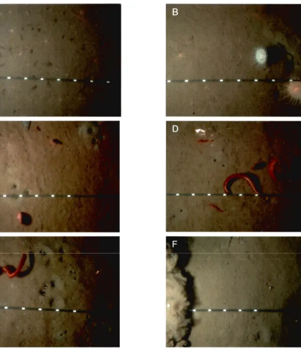
Figure 2: Representative photographs taken in the Estuary and Gulf of St. Lawrence in 2006 and 2007. A) Station 24: Ophiura sp. and detritus, B) Station 23: Ophiura sp., Actinauge sp. (right), Lycodes sp. (center right) in an imprint-depression and close to a medium burrow, C) Station 20: Small burrows, medium burrows with grey sediment (top right), double ploughs (from top left to down center), Pennatula aculeata (top center and down left), Amphiura sp. arms (top left) and flatfish (top center) 0) Station 19: Small and medium burrows, Pandalus sp., Pennatula borealis, P. aculeata and Amphiura sp. arms, E) Station 18: Small, medium and large burrows, imprints-depressions (top right), simple ploughs (down right and down left), P. aculeata, P. borealis and unknown crustaceans, and F) Station IC: Sediment cloud (Ieft), shrimp trail (down center to top right), imprints-depressions and Pandalus sp. Scale: 10 cm between two white lines.
28 80~---. C)' -60 E "0 c
----
èën
c 40 <D "0 E If),::
crs (J) '- 20 0 o 23 23S 24 19 20 CA CE 16 17 18 IC StationsFigure 3: Mean total organism density (ind. m-2 ± SE) for the 11 stations sam pied in the Estuary and Gulf of St. Lawrence in 2006 and 2007. Oxygen levels: hypoxic stations «20% O2) (black); oxy- stations (32-40% O2) (grey); oxy+ stations (>49% O2) (white).
1.3.1 Univariate analyses
The total-traces density (shown below as Mean ± SE) increased as the oxygen levels decreased; lower values were found at the oxy+ stations (3.12% ± 0.28), intermediate values at the oxy- stations (4.70% ± 0.46) and higher values at the hypoxic stations (7.47% ± 0.49) (Fig. 4A). The same pattern was observed for the surface-traces density (Fig. 48). Nested ANOVAs showed a significant difference of total and surface-traces densities for the different oxygen levels
oxy+ stations were significantly lower than hypoxic stations, and that ox
y-stations were not significantly different from oxy+ and hypoxic y-stations (Fig. 4A).
For the surface-traces density, Tukey's test showed that oxy+ and oxy- stations
were significantly lower th an hypoxic stations, and that oxy+ and oxy- stations were not significantly different from each other (Fig. 48).
The relief-traces density (Fig. 4C) was higher at the oxy- stations (1.14% ±
0.12), with high values for stations 19 and 20 (1.51% ± 0.17 and 1.71% ± 0.18,
respectively) and low values for stations CA and CE (0.80% ± 0.35 and 0.35% ±
0.03, respectively). This was followed by oxy+ stations (0.65% ± 0.08), with a low
value for station 17 (0.23% ± 0.03). The lowest relief-traces densities were found
at the hypoxic stations (0.63% ± 0.08), with the lowest value at station 24 (0.20%
± 0.05). Nested ANOVAs indicated no significant difference between the oxygen levels for relief-traces density (p>0.05, Table 3).
The density of grey-coloured sediment areas on the images (Fig. 40) was
higher at the oxy- stations (2.26% ± 0.43), with the highest values at stations 19
and 20 (3.21 % ± 0.81 and 4.41 % ± 0.87, respectively). However, oxy- stations
CA and CE had much lower values (0.23% ± 0.17 and 0.11 % ± 0.06,
respectively). Tukey HSO test within the oxy- group effectively revealed that the density of grey-coloured sediment areas at stations 19 and 20 were significantly higher th an at stations CA and CE (Fig 4D). The oxy+ stations had intermediate
30
values (0.78 %± 0.15) while the hypoxic stations had the lowest values (0.14% ± 0.08), with 0% for station 24. Nested ANOVAs indicated no significant difference between the oxygen levels for the density of grey-coloured sediment areas (p>0.05, Fig. 4D and Table 3).
The difference in means between stations within each oxygen level did not show a clear pattern for either surface, relief and total-traces diversities, nor for species richness, Pielou's evenness and Shannon-Wiener diversity (Fig. 4E-J).
Nested ANOV As indicated that oxygen levels were not significantly different for those indices (p>0.05, Table 3). However, nested ANOVAs indicated that stations within oxygen level were significantly different from each other for ail those indices (ail p<0.001; Table 3).
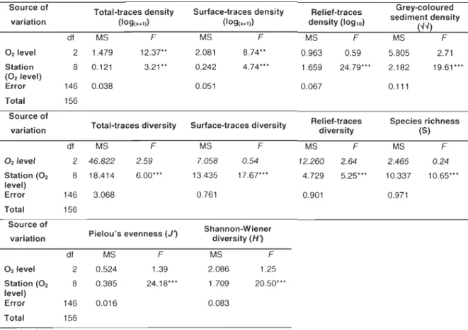
Table 3: Summary of nested ANOVAs for total-traces density (log(x+1)), surface-traces density (log(x+1)), relief-surface-traces density (loglO), grey-coloured sediment
density (-1-1), total-traces diversity, surface-traces diversity, relief-traces diversity, species richness (S), Pielou's evenness (J) and Shannon-Wiener diversity (H) to test the effect of oxygen level and station within oxygen level. Legend: ***
p<O.001, ** p<O.01, * p<O.05, NS.
Source of Total-traces density Surface-traces density Relief-traces Grey-coloured
sediment density variation (109(x+1)) (109(>+1)) density (10910) !-4-4) dl MS F MS F MS F MS F 021evel 2 1.479 12.37'* 2.081 8.74'* 0.963 0.59 5.805 2.71 Station 8 0.121 3.21** 0.242 4.74*** 1.659 24.79'** 2.182 19.61 '" (02Ievel) Error 146 0.038 0.051 0.067 0.111 Total 156
Source of Relief-traces Species richness
variation Total-traces diversity Surface-traces diversity diversity (S)
dl MS F MS F MS F MS F 021evel 2 46.822 2.59 7.058 0.54 12.260 2.64 2.465 0.24 Station (02 8 18.414 6.00'" 13.435 17.67**' 4.729 5.25*** 10.337 10.65**' level) Error 146 3.068 0.761 0.901 0.971 Total 156 Source of Shannon-Wiener
variation Pielou's evenness (J) diversity (H)
dl MS F MS F 02 1evel 2 0.524 1.39 2.086 1.25 Station (02 8 0.385 24.18*** 1.709 20.50' " level) Error 146 0.016 0.083 Total 156
A 10 ê ~
]
6 ~ ~ .,. 4 s .9 C..
2 " ::; D 6 l 5 ~ .~ ~ 4 c " E 3 ;; :il ~ 2 c ~ 1 " ::; A BHypo' O><y- O><y.
Oxygen levels A A B 2323$ 24 19 20 CA CE 16 17 18 te Stations G 5, - - - - -A-A- - - -A- . A,B A,B B A A B A,B
..
'.'.
2323$ 24 19 20 CA CE 16 17 lB le Stations B 10 l ~ 8 ,n c " '0 III 6 ~ ~ 4 't= " ~ c 2 '" " ::; E 12 ~ 10 "in ~ ;; ~ " ~ 6 S .9 4 C ~ ~ A Hypo' O><y- ChV' Oxygen levels A A A A A A A A,B B A,B B 23235 24 19 20 CA CE 16 17 la IG Stations H 5,---~ :il 4 g> .c .g 3 ~ " '~ l;l- 2 c ~ " ::; A B A A A A B,C B B A,C - A 2323524 19 20 CA CE 16 17 18 IG Stations J 1,8 ,---~ 1,6 A A ~ 1,4 ~ 1,2 ~ 1,0 .9 J:: 0,8 c ~ 0,6 ::; 0.4 A A " " B ,-A,B A,B A,B A,B B B 2323$ 24 19 20 CA CE 16 17 18 IG Stations C 2,0 ~ >- 1,5 -~ C " '0 ~ u 1,0 ~ i ~ c 0,5 " " ::; 0,0 F 4 >--~ ~ 3 ;; ~ " l;i " 2 ~i
C 1 ~ " ::; 1 1,0 0,8 0,6 0,4 A A A A B \ A,C C B B Bli
i
- ,~
ln
2323S24 1920 CA CE 1617 la le Stations A A B A,B B l A,B B A A B C , 23235 24 19 20 CA CE 16 17 18 le Stations A A AA,B A A , A,B A,B B B '.,.,
" 2323524 1920 CA CE 161718 te Stations 32Figure 4: Mean (± SE) of: A) total-traces density (%) and B) surface-traces
density (%) for three different oxygen levels, and C) relief-traces density (%), D)
grey-coloured sediment density (%), E) total-traces diversity, F) surface-traces
diversity, G) relief-traces diversity, H) species richness, 1) Pielou's evenness (J)
of total-traces and J) Shannon-Wiener's diversity index (H) of total-traces for
stations within oxygen level. Letters above columns indicate the results of Tukey HSD test between (A-B) and within (C-J) oxygen levels, where categories with
the same letter did not differ significantly. Oxygen levels: hypoxic stations «20%
Relationships between environ mental variables and univariate indices of bioturbation traces, and macrobenthic epifauna were examined using multiple linear regression models. The oxygen saturation is the variable that best explains the total and surface-traces densities (Table 4). The variability of total and surface-traces was explained by the oxygen saturation at 62% and 55%,
respectively (Table 4). We observed a decrease in total and surface-traces densities as the oxygen level increased (Fig. 5A and B). Environmental variables alone or combined never explained more than 53% of the other studied indices (Table 4). However, total organic matter and mean sediment grain size were often present as environmental variables explaining the regression models of the other indices. No multiple linear regression models could explain the species
34
Table 4: Results of the multiple linear regression models (stepwise procedure)
used to estimate total-traces density (%), surface-traces density (%), relief-traces
density (%), grey-coloured sediment density (-1-1) (%), total-traces diversity
(log lO), surface-traces diversity, relief-traces diversity, species richness, Pielou's
evenness (J) and Shannon-Wiener diversity (loge) (H) among the 11 stations
sam pied in the Estuary and Gulf of St. Lawrence in 2006-2007. Species richness
is not included in the table since no variables could explain these data.
Environmental variables in the regression models were depth (D, m), bottom
salinity (S, psu), bottom temperature (T, OC), bottom oxygen saturation (02, %),
total organic matter (TOM, %) and mean sediment grain size (MG S, Ilm). Note:
Underlined total organic matter was 10glO transformed for grey-coloured sediment
density (-1-1) and total-traces diversity (log lO) models. Partial ~ below each
regression coefficient; NS: not significant; ~: Total ~; Adj ~: Adjusted ~ and
MSE: Mean squared errors.
Total-traces density Partial ~ Surface-traces density Partial ~ Relief-traces density Partial ~
Grey sed density (1)1)
Partial ~ Total-traces div (10910) Partial ~ Surface-traces div Partial ~ Relief-traces diversity Partial ~ J' total-traces Partial ~ H' total-traces Partial ~ Intercept 0 (m) 9.55 NS 8.55 NS 0.16 0.01 0.25 -9.95 NS 0.40 NS S (psu) NS NS NS NS NS -305.79 -0.02 9.12 0.15 0.16 T <"C) NS O2 TOM (%) (%) -0.12 NS 0.66 MGS r2 (Adj r2) MSE (J.lm) NS 0.66 (0.62) 1.89 NS -0.12 NS NS 0.59 (0.55) 2.32 0.59 NS NS NS -0.13 0.44 (0.30) 0.17 0.19 NS -0.02 13.00 -0.08 0.66 (0.51) 0.08 0.19 0.34 0.13 NS NS NS 0.16 (0.07) 0.01 0.16 NS NS NS NS 0.31 (0.14) 2.89 -95.33 NS 3.05 -0.78 NS NS -0.09 0.67 (0.53) 0.10 0.39 0.11 0.17 -0.21 NS NS NS NS 0.12 -0.03 0.46 (0.32) 0.02 0.22 0.24 -0.59 NS NS NS NS 0.27 -0.06 0.47 (0.34) 0.08 0.24 0.23
10~---~ 8 2 A Total-traces (%) = 9.55 -0.12 * 02 (%)
•
R2 adj = 0.621 p= 0.002 10 20 30 40 50 60 70 Oxygen (% saturation) 10 .---~ 8 2 Surface-traces (%) = 8.55 - 0.12 * 02 (%)•
•
•
R2 adj = 0.546 P = 0.006•
O +---~--~--~~--~--~ 10 20 30 40 50 60 708
Oxygen (% saturation)Figure 5: Relation between oxygen saturation (%) and A) total-traces density (%)
and 8) surface-traces density (%) at the 11 stations sam pied in the Estuary and Gulf of St. Lawrence in 2006 and 2007.
1.3.2 Multivariate analyses
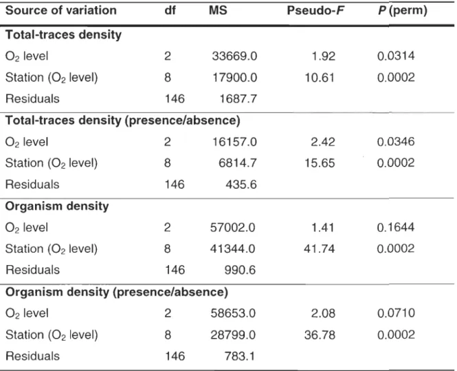
A clear difference between hypoxic and oxy+ stations was found with a non-metric multidimensional scaling (nMDS) plot of untransformed total-traces density data (Fig. 6A). The result was similar for nMDS plot of presence\absence-transformed total-traces density (Fig. 68). PERMANOVA analysis revealed that untransformed total-traces density between oxygen levels were significantly different (P = 0.0314, Table 5). Similar results were obtained when total-traces density were presence/absence-transformed (P
=
0.0346, Table 5). Pair-wise comparison test indicated that untransformed density data between hypoxic and oxy+ stations were significantly different (P=
0.0292). However, pair-wise comparison revealed no significant difference on36
presence\absence-transformed density data between the hypoxic and oxy+ stations (P
=
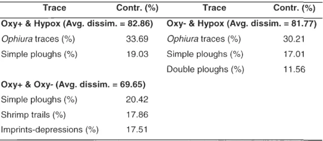
0.056). SIMPER analysis revealed that the Ophiura trace was contributing the most to the dissimilarity between the two oxygen levels at 33.69%, followed by the simple ploughs at 19.03% (Table 6).On the other hand, pair-wise comparison test on untransformed total-trace density revealed no significant difference neither between hypoxic and oxy-stations, nor between oxy+ and oxy- stations. PERMANOVA analysis also shows no significant difference in organism density between the oxygen levels, both for untransformed and presence\absence-transformed data (Table 5).
Table 5: Permutational analysis of variance (PERMANOVA) (Anderson, 2001;
McArdle & Anderson, 2001) results testing the effect of oxygen level and its
interaction with total-traces and organism densities based on Bray-Curtis similarity matrices performed on untransformed and presence\absence transformed data.
Source of variation df MS Pseudo-F P(perm)
Total-traces density
021evel 2 33669.0 1.92 0.0314
Station (02 level) 8 17900.0 10.61 0.0002
Residuals 146 1687.7
Total-traces density (presence/absence)
021evel 2 16157.0 2.42 0.0346 Station (02 level) 8 6814.7 15.65 0.0002 Residuals 146 435.6 Organism density 021evel 2 57002.0 1.41 0.1644 Station (02 level) 8 41344.0 41.74 0.0002 Residuals 146 990.6
Organism density (presence/absence)
021evel 2 58653.0 2.08 0.0710
Station (02 level) 8 28799.0 36.78 0.0002
38
Table 6: Results of similarity percentage analyses (SIMPER) showing the
contribution (%) of the types of traces to the average Bray-Curtis dissimilarity of
compared oxy+, oxy- and hypoxic groups as weil as the average dissimilarity (%)
among groups.
Trace Contr. (%)
Oxy+ & Hypox (Avg. dissim.
=
82.86)Ophiura traces (%) 33.69
Simple ploughs (%) 19.03
Oxy+ & Oxy- (Avg. dissim.
=
69.65)Simple ploughs (%) 20.42
Shrimp trails (%) 17.86
Imprints-depressions (%) 17.51
Trace Contr. (%)
Oxy- & Hypox (Avg. dissim.
=
81.77) Ophiura traces (%) 30.21Simple ploughs (%)
Double ploughs (%)
17.01
A x 2OS.ess:O.22 B o o o o o o o 20 Svess: 021 o x o 0x X 0 o Sbo o 0 0 ~~ 0 0 o 0 0 X'*'" ~ ~ 8 X o XX x~:p ~%
î
o 0 00 x 0 ,p 0 ,èfuo'''''S< (): X 0 DO ODC xCII x <lJ x ,p 0 o 'fi x o o o XFigure 6: Non-metric multi-dimensional scaling (nMDS) plots of total-traces density per oxygen level based on A) untransformed data and B) presence\absence transformed data. Oxygen levels: hypoxic stations (0); oxy-stations (x); oxy+ oxy-stations (0).
40
1.4 Discussion
1.4.1 Macrobenthic epifauna
The results of this study indicate that the decreasing oxygen concentrations in the EGSL bottom waters has not yet lead to a decrease in macrobenthic species richness, which is contrary to our expectations. This observation does not appear to support previous studies conducted on the effects of hypoxia in other parts of the world (Diaz & Rosenberg, 1995; Wu, 2002; Diaz & Rosenberg, 2008). However, it has been reported that, under hypoxic conditions, suspension feeders are generally replaced by deposit feeders (Diaz &
Rosenberg, 1995; Wu, 2002). Even if the statistical analyses presented here do not show significant differences in species richness between the different oxygen levels, our results could indicate recent changes of the macrobenthic epifauna community structure in the hypoxic zone of the EGSL, where suspension feeders and low-oxygen intolerant species have been replaced by deposit feeders and low-oxygen tolerant species. First, the species with the highest density and abundance, the deposit feeding, low-oxygen tolerant Ophiura sp. (Vistisen & Vismann, 1997), was only found at the hypoxic stations 23 and 24. Second, SIMPER analyses showed that the Ophiura trace contributed most to the difference between the hypoxic and the oxy+ stations. Third, the highest density of the suspension feeder P. aculeata at oxy- stations 20 and CA and the limited