HAL Id: hal-02141286
https://hal.archives-ouvertes.fr/hal-02141286
Submitted on 27 May 2019
HAL is a multi-disciplinary open access
archive for the deposit and dissemination of
sci-entific research documents, whether they are
pub-lished or not. The documents may come from
teaching and research institutions in France or
abroad, or from public or private research centers.
L’archive ouverte pluridisciplinaire HAL, est
destinée au dépôt et à la diffusion de documents
scientifiques de niveau recherche, publiés ou non,
émanant des établissements d’enseignement et de
recherche français ou étrangers, des laboratoires
publics ou privés.
Methodology for optimal wind vane design
Hugo Kerhascoet, Johann Laurent, Audrey Cerqueus, Marc Sevaux, Eric
Senn, Frederic Hauville, Raphael Coneau
To cite this version:
Hugo Kerhascoet, Johann Laurent, Audrey Cerqueus, Marc Sevaux, Eric Senn, et al.. Methodology
for optimal wind vane design. OCEANS 2016 - Shanghai, Apr 2016, Shanghai, China. pp.7.
�hal-02141286�
Methodology for Optimal Wind Vane Design
Hugo Kerhascoët
Lab-STICC and IRENav Université de Bretagne Sud
nke Marine Electronics Email: [email protected]
Johann Laurent and Audrey Cerqueus
and Marc Sevaux and Eric Senn
Lab-STICC Université de Bretagne Sud Email: [email protected]
Frédéric Hauville
and Raphaël Coneau
M2EN
Institut de Recherche de l’Ecole Navale Email: [email protected]
Abstract—Measurements of wind direction are sought after by a multitude of professionals in many different domains. Whether to recalibrate meteorological models or simply for leisure activities, the demand for accurate and responsive wind measurements is widespread. This study was motivated by the need to improve the responsiveness of direction measurements on yachts. Here we argue that the ideal form factor of the wind sensor can be determined using digital tools, rather than empirically, with the aim of improving the mechanical response of the wind vane. Then we present the results obtained by applying a predictive filter method tailored to the specified form factor. We have developed and experimentally validate a mathematical model describing the dynamic behavior of a wind vane. This model is then used to determine the form factor of the vane that will give the best possible response to perturbations it will encounter. To do so we use operational research tools, specifying the mechanical characteristics of the vane and by providing the future use conditions of the sensor, in the form of a wind speed spectral density. The design built from this optimization methodology helps reduce the response time of the vane by 44% compared to to designs currently in use.
We then work on digital signal processing by using a predictive filter which takes into account the dynamic characteristics of the vane previously determined by the mathematical model. This step vastly improves the quality and sensitivity of the signal, leading to another reduction in response time of 83%. This brings the total decrease in response time at 90%.
There is therefore not only an improvement in the quality of wind direction measurements, but also with respect to the set of data that is derived from this information. In the context of single-handed racing boats, the performance of the automatic pilot directly benefits from this improvement in responsiveness.
NOMENCLATURE
ωn Natural frequency, rad/s.
ωp Damped natural frequency, rad/s.
ζ Damping ratio.
β Current position of the vane. γ Apparent wind direction. Cr Bearing dry friction.
I Moment of inertia. U Wind speed, m/s. ρ Air density.
S Wing platform area.
xA Aerodynamic point of application.
xG Gravity center to rotation axis distance.
K Lift coefficient. T r Response time.
A, B, C, L, H Dimensions characterizing the vane.
Apparent wind Wind experienced by an observer in motion. True wind Wind relative to a fixed point.
I. INTRODUCTION
Measurements of wind direction are sought after by a multitude of professionals in many different domains. Whether to recalibrate meteorological models or simply for leisure activities, the demand for accurate and responsive wind mea-surements is widespread. This study was motivated by the need to improve the responsiveness of direction measurements on yachts. Such sought-after performance gains will not only ben-efit human skippers, but also automatic pilot systems, which use wind direction as a source of information. The current wind vane specifications used on yachts have been derived empirically and do not meet modern performance standards. Improvements are both mechanical and relate to better signal processing. Here we argue that the ideal form factor of the wind sensor can be determined using digital tools. The initial goal is to improve the mechanical responsiveness of the vane. Beyond that, an optimised design could significantly improve signal quality. This paper describes the methodology and tools that were used to specify the optimal form factor. Finally, we present the results obtained by applying a predictive filter method tailored to the specified form factor.
II. METHODOLOGY STEPS DESCRIPTION
A. Overall Diagram
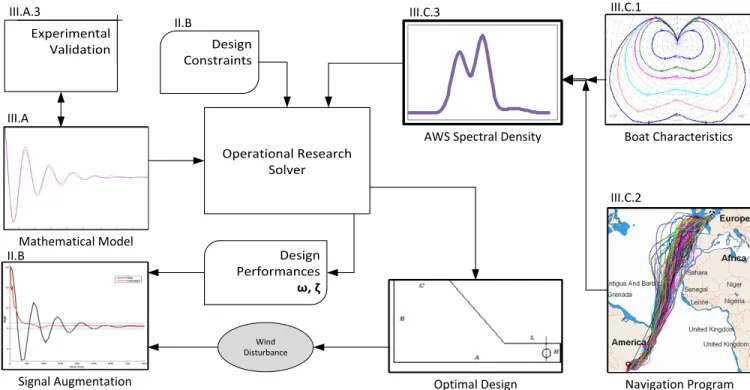
The overall process for the optimization of the vane de-scribed in this article is summarised in Figure 1. This diagram shows the various steps (and their interactions) that contributed to the specification of the solver’s input data. It should be noted than both performance and design are a function of physical characteristics (including the mathematical description) of the sensor (materials, bearings) and the strength of the wind it is exposed to-therefore, boat characteristics and its sailing programme. The solver outputs the optimal form factor and associated performance criteria. These can then be used as input data for the final step: signal processing (IV-B). B. Operational Research
The methodology is based on the solver and uses operational research methods. This tool takes the input data, models the behaviour of the element to be optimized, and provides an optimal solution for the question being asked. Operational
AWS Spectral Density Mathematical Model Boat Characteristics Navigation Program Wind Disturbance Optimal Design
III.A.3 III.C.3 III.C.1
III.C.2
II.B III.A
II.B
Signal Augmentation
Fig. 1. Overview of the optimization process showing the solver’s input data and the procedure for obtaining them. Also shown is how the final design and performance criteria are used.
research is not the subject of this paper; here we only provide a high-level description. As the mathematical formulation is non-linear, the problem is resolved using two specialized solvers: LocalSolver [1] takes a heuristic approach, while Ibex [2] is an exact solver. This step is described in Cerqueus et al. [3]. Here, the solver must provide the optimal dimensions for a vane that meets the requirements of the mathematical model (III-A) characterizing its dynamics.
C. Input Data
To function, the solver need equations that model the problem (III-A), and the environment in which the product will be used (III-C). Finally the tool must be provided with the parameters to be optimised as a function of how the signal will be used (III-D), while at the same time specifying physical design constraints (III-B).
D. Output Data
The tool must provide the optimal form factor of the vane by specifying the dimensions shown in Figure 2. Just as important, the tool must also provide performance data (char-acterized by ωp and ζ) if they are used in signal processing
(IV-B).
III. INPUTDATA
This section describes the principal solver data. A. Mathematical model
1) Challenges: Section II-C highlighted the need for a mathematical model that describes wind vane dynamics. This
B C
H L
A
Fig. 2. Dimensions of the vane. A, B, C, L and H are output parameters that the solver uses to define the form factor. The circle represents the fixation point of the vane on the axis (- - -) that enables rotation.
was the first challenge. The goal was to make a link between the physical characteristics of the vane, i.e. dimensions, weight, bearings, and its dynamics when exposed to wind pertubations. We were not looking for an absolutely precise model, but one that was good enough for the digital solver to determine the optimal design. The acceptable margin of error was set at 10%.
2) Equations: Many approaches have been adopted in the literature to model the behaviour of a weather vane but, in general terms, the angular response when exposed to wind can be assimilated to the response of a second-order system [4]. This result can be found in applying the fundamental principle of dynamics to the wind vane system. The second-order linear differential equation with constant coefficients takes the form:
¨
β + 2ωpζ ˙β + ωp2β = ωp2γ −
Cr
I (1)
Where β is the angular position of the vane and γ is the apparent wind direction.
In the framework of this study, the link between the physical parameters of the vane (form, density, etc.) and the coefficients of the differential equation make it possible to use the solver. As shown in Figure 3, the system’s damped natural fre-quency ωpand its damping ratio ζ are sufficient to specify the
step response of a second-order system. ωpdefines the angular
frequency of the response and ζ is the transitional regime: it is overdamped if ζ > 1 or underdamped if 0 < ζ < 0.7.
The mathematical model can be summarised by equations (2) and (3): ωn= U r ρSxAK 2I (2) ζ = xG 2 r ρSxAK 2I (3) ωP = ωn p 1 − ζ2 (4)
These equations constitute the link between the physical dimensions of the vane, Figure 2, and ωp,ζ. They are therefore
sufficient to define its behaviour.
It should be noted that ωp is proportional to wind speed U
and that ζ is a constant as it only depends on the physical characteristics of the vane. S is the wind platform area; xA
and xG are respectively the aerodynamic point of application,
and the distance between the centre of gravity and the rotation axis. I is the moment of inertia and K is the lift
Fig. 3. Step response of a second-order system. The step response is the same for the three signals that are shown, only one of the parameters of the pair (ω, ζ) governing the differential equation differs. The signals (- - -) and (—) have the same damping ratio ζ but frequency ω is higher for (- - -). Both (—) and (-.-) have the same frequency, but ζ is higher for (-.-).
-20 -15 -10 -5 0 5 10 15 20 25 30 0 0,5 1 1,5 2 2,5 3 3,5 4 4,5 5 mo d el in g err o r (%) Aspect Ratio
ζ
ω
Fig. 4. Percentage errors between frequency ω and damping ratio ζ estimated by the model and results obtained in wind tunnel tests. Data are classified as a function of the aspect ratio of the design.
coefficient with respect to the angle of incidence of the vane γ. 3) Experimental validation: The model describing the link between the dimensions of the vane and its natural frequency ωn, together with damped frequency ζ, was empirically tested
in a wind tunnel. Seventeen designs, with different aspect ratios and a variety of potential configurations were tested in various wind strengths. Figure 4 shows the results precison. It should be noted that for extreme aspect ratios (lower than 1 or higher than 3.5) the damped ratio and frequency error were significant. On the other hand, with respect to the range of aspect ratios [1; 3.5] the modelling error is acceptable given the use cases. Errors were of the order of [−3; 2.3]% for frequency and [−3; 9]% for the damping ratio. In practice, we were looking to determine a form factor and not intrinsic performance, therefore this degree of precision was considered satisfactory.
B. Design constraints
Section III-A3 highlights that the model was only consid-ered to be satisfactorily accurate for the range of aspect ratios [1; 3.5]. The solver did not therefore suggest designs beyond this range. The dimensions characterizing the form factor of the vane A, B, C, L, and H are bounded in size in order to ensure that the vane can actually be made. In practice, the solver was never limited by these constraints as they are big enough from the point of view of the proposed designs. The density of the vane material, its thickness, together with the dry friction coefficient of bearings Cr, constituted other constraints.
Destructive testing showed that vibrations created by the vane as it resonated with its support led to material failure. The frequency of this resonance was identified and the de-signs proposed by the solver were required to be below the frequency ωmax.
C. Apparent wind speed spectral density
Equation (2) shows that the frequency of the vane is a function of wind speed U . It is therefore important to take into account the strength of the wind at sea. Wind speeds are represented as a spectral density, which specify the temporal division of perceived speeds rather than just minimum and maximum values.
The spectral density of apparent wind is an input to the solver. This makes it possible to select a design that is optimised for a spectral density that represents the distribution of wind speeds that the sensor will encounter, rather than a given or steady wind speed.
The modelled wind sensor is expected to be mounted onto a yacht. As these boats move, the apparent wind it records is therefore a combination of the true wind, and the wind created by the movement of the vessel.
To determine the range of apparent wind, it is necessary to take into account the speed of the boat (III-C1) and true wind speeds it will encounter during his sailing journey (III-C2).
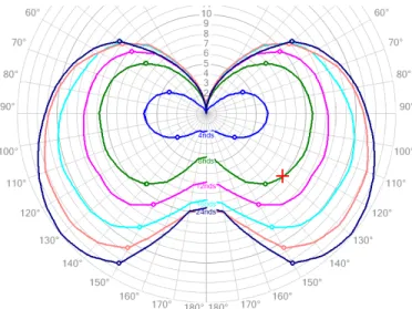
1) Speed polar: There are a multitude of sailing boats, from pleasure craft to competition yachts, and performance means something different to each of them. The performance of a sailing boat is most often represented in the form of a polar speed diagram (Figure 5). This diagram shows the speed of a boat as a function of the angle that it makes with the true wind. Each curve represents a true wind strength.
Polar plots are not the focus of this article. Polar speed is approximated by digital design tools used by naval architects, then refined by the skipper in the course of their journey. In general, bespoke tools such as Adrena are used [5]. Adrena was used to construct the polar diagram and develop the routings described in the following paragraph.
Fig. 5. Polar plot for an IMOCA60. Potential speed for corresponding wind strength is shown as a function of the angle of the true wind. The point marked with a cross is understood as follows: for a true wind speed of 8 knots and for a boat at 130◦to this wind, a speed of 10 knots can be expected.
2) Sailing programme: Users do different things with their boats (inshore racing, the America’s Cup, offshore racing, etc.) and therefore do not experience the same weather conditions. Furthermore, in offshore racing the conditions that are encoun-tered vary as a function of the race. Very different conditions are encountered in races such as the Transat, the Vendée Globe or the North Atlantic record. We used meteorological routing software [5] to estimate the apparent wind that a boat might encounter during a race, given a specific route. This software calculates the route that should be taken as a function of the boat’s characteristics (polar speed) and weather conditions. The operation is performed hundreds of time using meteorological records from previous years (for example the past ten) on a given date of departure ± several days. This technique provides a set of statistical routings (Figure 6) that includes meteorological conditions and the speed of the boat at all times. From this, we can deduce apparent wind speed, and therefore the statistical distribution (Figure 7), as a percentage, of the wind speeds the sensor may encounter during the race.
Fig. 6. Statistical routings for the Jacques Vabres 2015 race for an IMOCA60. Calculations are based on meteorological data for the past 10 years for 150 departure dates with a range of ±7 days.
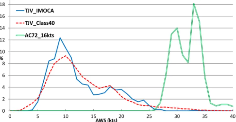
3) Spectral density: Examples of apparent wind speed (AWS) spectral densities obtained from an exhaustive number of statistical routings are shown in Figure 7. The graph highlights two features: first, for the same race (in this case the Transat Jacques Vabres 2015) the spectral densities of two fairly similar boats (Class40 and IMOCA60) are sufficiently different to justify a dedicated optimization process. The second feature is the large difference between the spectral
0 2 4 6 8 10 12 14 16 18 0 5 10 15 20 25 30 35 40 % AWS (kts) TJV_IMOCA TJV_Class40 AC72_16kts
Fig. 7. Spectral densities for two different boats (Class40 and IMOCA60) in the same race (Jacques Vabres 2015). The third is for an AC72 in 16 knots of true wind.
densities of offshore racing boats and the AC72 (an Amer-ica’s Cup boat). This is explained by their radically different performance and sailing programmes. The value of using spectral density rather than perceived minimum and maximum values of a homogenous wind is that in the second case, the form factor would be optimised for the whole range, while in practice extreme values are not encountered very often. Even worse, in the case of the AC72, which has two distinct and symmetric peaks on either side of a central value, basing calculations on a homogeneous range (i.e. a flat spectral density) will produce a design that is optimised for the central value, while this is not the point at which the spectral density is highest, in fact the opposite is the case.
Measuring the spectral density makes it possible to estimate the maximum speed of the apparent wind that the vane will be exposed to; this information is used in the constraint ωmax.
D. Use cases
The variables to be optimized will depend on how the signal will be processed and the expected use. Classical signal processing uses the raw signal (potentially with the addition of an averaging filter) and response times must be optimized. In other words, it is necessary to minimize T r in equation (5), which is the function of ωn and ζ. This is because the lower
T r, the better the responsiveness of the system.
T r(5%) = −ln(0.05) ζωn
(5)
In the second use case, the signal is processed by a pre-dictive algorithm. This method is explained in section IV-B. In this case we seek to optimize the behaviour of the vane that makes the filter converge the quickest, in other words the frequency must be maximized. In practice, the filter’s convergence time is proportional to the period of the system (see Figure 10). At the same time, the frequency must be within ωmax.
IV. OUTPUTDATA
A. Results
Optimal performance characteristics are shown in Figure 8. The response time best represents the quality of the design; the faster this time, the better the signal information.
Four designs are shown in Figure 8:
• nkeV1, was the initial design. It should be noted that for the specified range of wind [4; 23]m/s, frequency ex-ceeds ωmax. In this case, resonance was causing material
damage.
• nkeV2, was also specified empirically. Here, the aim was to eliminate resonance and keep the frequency below ωmax. Performance, in terms of response time, is only
slightly improved.
• B&G, is from another manufacturer in a very difference
performance domain; responsiveness is poorer, and re-sponse time is also slow.
• Optimal, is the design arrived at by the application of
the methodology described in this article. Response time T r is very low compared to nkeV2 (by 44%), while performance (in terms of frequency) is not degraded and remains below ωmax.
• Kalman, is not strictly a design, but an improved version that employs the signal processing method onto the Optimal design. An explanation is provided in section IV-B.
In addition to performance, the solver outputs the vane pro-file. The one that was obtained using the described procedure (Optimal), is shown in Figure 9, superimposed on the profile of previou design (nkeV2).
The materials used for the design of the two vanes are strictly identical, performance gains are solely the result of different form factors. The optimized vane has a higher aspect ratio and the surface is slightly raised. However, most importantly,
0 20 40 60 80 100 0 0,5 1 1,5 2 2,5 3 ω Tr 5% (sec) nkeV1 nkeV2 B&G Optimal Kalman ωmax 4m/s 23m/s
Fig. 8. Performance comparison for old-style vanes and the new, optimised design. Frequency and response times are given for a wind range [4; 23]m/s. The optimal performance zone is found in the top-left of the figure. The horizontal line represents the maximum frequency ωmaxbefore mechanical
141 64 L = 25 20 nkeV2 Optimal
Fig. 9. Superposition of old (nkeV2) and new (optimised) vane designs. Sizes in millimetres.
the lifting surface is offset with respect to the axis of rotation by the tab L that acts as a shaft. It is this feature that makes it possible to move the aerodynamic centre xA back, while
maintaining a moderate moment of inertia compared to a delta design (without shaft).
B. Signal Augmentation
The final task concerned signal processing. Here we look at the best way to processes the digital signal produced by oscillations of the wind vane. Section III-A showed that the vane acts as a second-order system. This being the case, it is reasonable to implement equation (1) governing its dynamics in a predictive, Kalman-type filter [6]. The method is fairly complex and here we simply present the results, the details will be the subject of a future article.
An initial attempt to integrate the characteristics governing wind vane dynamics is presented in Pinsker [7] in the field of aviation. Our approach is different to the extent that Pinsker only characterizes expected errors as a function of perturbations. The technique described here makes it possible to both recover from any delays and catch mechanical errors. The sensor’s bandwidth is therefore extended and the signal is more accurate.
As ωp and ζ are provided by the solver, β corresponds to
the current position of the vane and γ is the parameter to be estimated using the predictive filter.
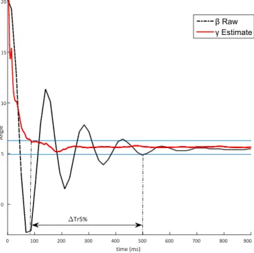
The result of applying the filter to the optimized design is shown in Figure 10. The vane is exposed to a 14◦perturbation in a wind tunnel and oscillation β is recorded and fed into the predictive filter. The two horizontal lines represent a 5% margin of error. Consistent with the model’s predictions for a 10m/s wind - and as shown in Figure 8 - β is within the 5%
time (ms) 0 100 200 300 400 500 600 700 800 900 Angle ° 0 5 10 15 20 "Tr5%
Fig. 10. Step response recorded in a wind tunnel with a wind of 10m/s. Comparison of the raw signal β and the estimate of the direction of the perturbation γ by the predictive filter. The two horizontal lines represent a 5% error margin. The gain in response time is shown by the two vertical lines.
error margin after 500ms.
Despite the fact that the estimate of the direction of the per-turbation γ provided by the predictive filter is not initialized, it converges in the 5% band in 90ms. This is only 18% of the time normally needed. The performance obtained with this signal processing method is included in Figure 8, where it can be seen that the improvement is considerable.
V. CONCLUSION
The methodology presented here offers a solution to the poor responsiveness of mechanical sensors used to detect wind direction. With the aid of digital tools, it specifies the optimal form factor for a vane that takes into account the stresses it will encounter. This optimized design offers more than 40% gain in response time compared to designs currently in use. Furthermore, the addition of a predictive signal processing step that takes account of vane dynamics vastly improves the quality and sensitivity of the signal, leading to another gain in response time of over 80%. There is therefore not only an improvement in the quality of wind direction measurements, but also with respect to the set of data that is derived from this information. In the context of single-handed racing boats, the performance of the automatic pilot directly benefits from this improvement in responsiveness.
The methodology described here could be applied to any type of activity where the spectral density of wind is relevant.
REFERENCES
[1] “Localsolver.” [Online]. Available: http://www.localsolver.com [2] “Ibex.” [Online]. Available: http://www.ibex-lib.org
[3] A. Cerqueus, M. Sevaux, H. Kerhascoet, and J. Laurent, “Modelisation de la girouette d’un voilier : experimentation avec LocalSolver,” in ROADEF: Recherche Operationnelle et d’Aide a la Decision, Compiegne, France, Feb. 2016. [Online]. Available: https://hal.archives-ouvertes.fr/hal-01275944
[4] P. Ebert and D. Wood, “On the dynamics of tail fins and wind vanes,” Journal of Wind Engineering and Industrial Aerodynamics, vol. 56, pp. 137–158, may 1995.
[5] “Adrena.” [Online]. Available: http://www.adrena.fr/
[6] R. E. Kalman, “A New Approach to Linear Filtering and Prediction Problems,” Journal of basic Engineering, vol. 82, no. Series D, pp. 35–45, 1960.
[7] W. Pinsker, “The Static and Dynamic Response Properties of Incidence Vanes with Aerodynamic and Internal Viscous Damping,” Ministry of Aviation, Tech. Rep. 652, 1963.