Sensitivity calculations and variance analysis in plant measurement reconciliation

SENSITIVITY CALCULATIONS AND VARIANCE ANALYSIS

IN PLANT MEASUREMENT RECONCILIATION

G. HEYEN 1, E. MARECHAL 2, B. KALITVENTZEFF 1, 2

1 : Laboratoire d'Analyse et Synthèse des Systèmes Chimiques, Université de Liège Sart Tilman B6A, B-4000 Liège (Belgium)

2 : BELSIM s.a., Allée des Noisetiers 1, B-4031 Angleur (Belgium)

Abstract - Analysis of the results of a data reconciliation program is made easier by extracting more information from the Jacobian matrix of the constraint equations. Standard deviation for all state variables (measured or not measured) is related to the standard deviation of measurements. Distinction between variables that are actually corrected by the validation process, and those that are merely derived from a single measurement is straightforward. Based on this information, decisions can be taken : deletion of unnecessary measurements, addition of new measurement points and their optimal selection, or identification of key measurements for which any enhancement of accuracy would result in significant improvement in the quality of the process validation.

SCOPE

Plant data reconciliation has been developed for a long time (Kalitventzeff (1978), Gosset (1980) and has been transposed with success from academic to industrial applications. It has proven to be a valuable tool in processing raw measurements collected in operating plant, and is now being linked to real time data logging systems (Kalitventzeff (1991).

However results of validation programs can be difficult to interpret. For instance, when a measured variable is not (much) corrected, does it mean that the measurement is reliable, or does it results from a lack of redundancy in a measurement subset, such that no other experimental value can influence the value of the state variable ? In fact, a common mistake in assessing the benefit of data reconciliation is to believe that all variables that are not significantly corrected (e.g. less than twice the standard deviation of the experimental value) are reliable, and that a large redundancy in the measurement set results necessarily a reliable estimate for all state variables.

Obviously, a procedure to assess the accuracy of the validation results leads to a better knowledge of the key process variables. Rules to select optimal measurement points can also be derived from the sensitivity matrix of the model equations used as constraints in the data reconciliation problem.

MATHEMATICAL DEVELOPMENT :

The validation problem can be expressed as a constrained minimization problem. The following development assumes that constraints are linear or have been linearized :

min (X-X')T W (X-X') (1)

X,Y

s.t. A X + B Y + C = 0

The constrained problem can be transformed into an unconstrained one using Lagrange formulation :

min L = (X-X')T W (X-X') + 2 λT (A X + B Y + C) (2)

X,Y,λ

Stationarity conditions are : This leads to following equation system : dL dX = 0 W X + AT λ = W X' dL dY = 0 BT λ = 0 (3) dL dλ = 0 A X + B Y = - C

One can thus define a square matrix M (size m+n+p), an array V and an array D, such that :

M =

[

]

W 0 A

0 0 B

A B 0

V =

[]

X

Y

λ

D =

[ ]

W X '

0

- C

V = M-1 D (5)

Matrix M-1 is the sensitivity matrix : both X and Y arrays appears as linear combinations of measured values X'. The sensitivity matrix allows thus to evaluate how the validated value of a variable depends from all measured variables and their standard deviations. In particular :

Xi = j=1 m+n+p ( M-1 )i j Dj = j=1 m ( M-1 )i j Wjj X'j - k=1 p ( M-1 )i n+m+k Ck (6) Yi = j=1 m+n+p ( M-1 )n+i j Dj = j=1 m ( M-1 )n+i j Wjj X'j - k=1 p ( M-1 )n+i n+m+k Ck (7)

The variance of a linear combination Z of several variables Xj is calculated as follows : Z = j=1 m aj Xj (8) var(Z) = j=1 m aj2 var(Xj) (9)

Thus one obtains the following estimate for the variance of validated measured variables : var(Xi) =

j=1 m

{( M-1 )i j Wjj}2 var(X'j) (10)

and for the estimated unmeasured variables : var(Yi) =

j=1 m

{( M-1 )n+i j Wjj}2 var(X'j) (11)

Previous expressions can be simplified by taking into account that :

var(X'j) = 1 / Wjj (12) thus : var(Xi) = j=1 m ( M-1 )i j2 / var(X'j) (13) var(Yi) = j=1 m ( M-1 )n+i j2 / var(X'j) (14)

ILLUSTRATION

As a first example, let us a consider a simplified flowsheet for an ammonia synthesis loop (figure 1). Pressure drops in the reactor from 280 to 270 bar, which is compensated by the recycle compressor; no pressure drop is assumed in other units. Measured values are displayed on the flowsheet.

W3 F05 F06 F07 RCTIN Q2 RCTOUT FLV Q3 FL FV PURGE RECYC T=40°C T=25°C T=30°C T=19°C T=20°C F=3.2t/h T=378°C F=77 t/h T=540°C T=20°C F=63 t/h W=330 kW F=12.5 t/h 0.1% CH4 0.3% Ar 97.8% NH3 1.3% H2 0.5% N2 0.3% CH4 3.7% Ar 5.4% NH3 67.1% H2 23.5% N2 0.2% CH4 4.8% Ar 7.2% NH3 64.4% H2 23.4% N2

Figure 1. Simplified flowsheet of an ammonia synthesis loop : measurements available for data reconciliation

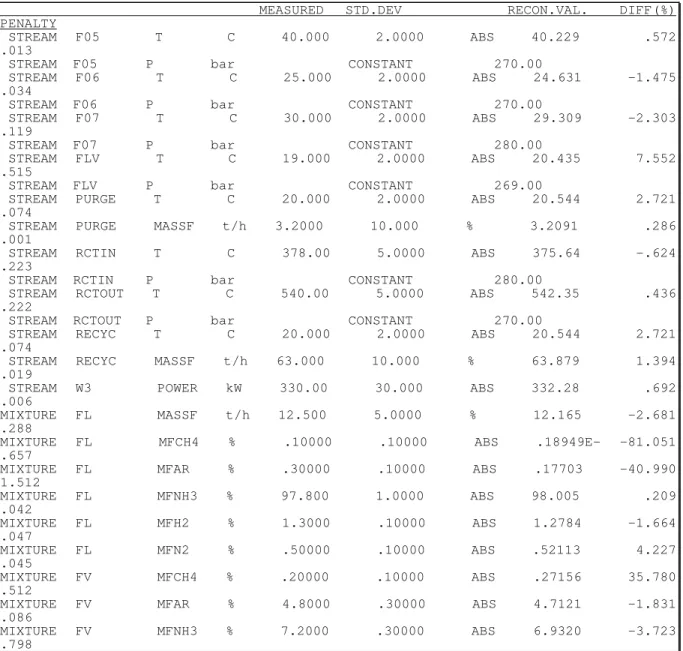
Table 1 : results of data reconciliation

MEASURED STD.DEV RECON.VAL. DIFF(%) PENALTY

STREAM F05 T C 40.000 2.0000 ABS 40.229 .572 .013

STREAM F05 P bar CONSTANT 270.00

STREAM F06 T C 25.000 2.0000 ABS 24.631 -1.475 .034

STREAM F06 P bar CONSTANT 270.00

STREAM F07 T C 30.000 2.0000 ABS 29.309 -2.303 .119

STREAM F07 P bar CONSTANT 280.00

STREAM FLV T C 19.000 2.0000 ABS 20.435 7.552 .515

STREAM FLV P bar CONSTANT 269.00

STREAM PURGE T C 20.000 2.0000 ABS 20.544 2.721 .074

STREAM PURGE MASSF t/h 3.2000 10.000 % 3.2091 .286 .001

STREAM RCTIN T C 378.00 5.0000 ABS 375.64 -.624 .223

STREAM RCTIN P bar CONSTANT 280.00

STREAM RCTOUT T C 540.00 5.0000 ABS 542.35 .436 .222

STREAM RCTOUT P bar CONSTANT 270.00

STREAM RECYC T C 20.000 2.0000 ABS 20.544 2.721 .074

STREAM RECYC MASSF t/h 63.000 10.000 % 63.879 1.394 .019

STREAM W3 POWER kW 330.00 30.000 ABS 332.28 .692 .006

MIXTURE FL MASSF t/h 12.500 5.0000 % 12.165 -2.681 .288

MIXTURE FL MFCH4 % .10000 .10000 ABS .18949E- -81.051 .657

MIXTURE FL MFAR % .30000 .10000 ABS .17703 -40.990 1.512 MIXTURE FL MFNH3 % 97.800 1.0000 ABS 98.005 .209 .042 MIXTURE FL MFH2 % 1.3000 .10000 ABS 1.2784 -1.664 .047 MIXTURE FL MFN2 % .50000 .10000 ABS .52113 4.227 .045 MIXTURE FV MFCH4 % .20000 .10000 ABS .27156 35.780 .512

MIXTURE FV MFAR % 4.8000 .30000 ABS 4.7121 -1.831 .086

MIXTURE FV MFNH3 % 7.2000 .30000 ABS 6.9320 -3.723 .798

MIXTURE FV MFH2 % 64.400 1.0000 ABS 64.871 .731 .221

MIXTURE FV MFN2 % 23.400 1.0000 ABS 23.214 -.796 .035

MIXTURE RCTIN MASSF t/h 77.000 10.000 % 79.253 2.925 .086

MIXTURE RCTIN MFH2 % 67.100 1.0000 ABS 66.849 -.374 .063

MIXTURE RCTIN MFCH4 % .30000 .10000 ABS .22207 -25.978 .607

MIXTURE RCTIN MFAR % 3.7000 .30000 ABS 3.8389 3.755 .214

MIXTURE RCTIN MFNH3 % 5.4000 .30000 ABS 5.5084 2.007 .130

MIXTURE RCTIN MFN2 % 23.500 1.0000 ABS 23.582 .348 .007

Standard deviation is set to 10% of measured value for gas flowrates, and to 5% for liquid product. It is 2°C for temperatures below 100°C, and 5°C above. Standard deviation for compressor power is 30kW. It is set to 0.1 mole% for mole fractions below 2%, to 1 mole% for mole fractions above 20%, and to 0.3 mole% otherwise. The reconciliation problem involves 28 measurements, 33 unmeasured state variables, 50 constraint equations, and thus 17 redundancies. 10 variables are considered as constants (all pressures). Measurements appear to be acceptable, since none is corrected by more than twice the assumed standard deviation, as shown in the results (table 1). Knowing the variance of validated variables allows to detect the respective importance of all measurements in the state identification problem. In particular, some measurements might appear to have little effect on the result, and might thus be discarded from analysis. Some measurements may appear to have a very high impact on the validated variables and on their variance : these measurements should be carried out with special caution, and it may prove wise to duplicate the sensors.

The sensitivity analysis module generates two types of reports. The first one contains for each measurement the measured value and the reconciled value, the assumed accuracy (standard deviation) of the measurement (Abs.Acc.) and the a posteriori accuracy of the reconciled data; these figures are also as percentage of the corresponding value (Rel.Acc.). All state variables depending from a given measurement are also listed, with the weight factor (Contrib.) indicating the contribution of the measurement variance to the variance of the reconciled value. The second type of report contains the same information, but sorted by state variable : for each variable, one obtains the list of the most important measurements used to estimate its value.

The following example illustrates the content of the first report type. Information listed is related to the measurement of ammonia mole fraction in stream FL, identified by tag name FL1_MFNH3. This value has been corrected from 97.80 mol% to 98.005 mol%. Standard deviation of validated value is 0.121 mol% (0,12% of validated value), significantly lower than the measurement standard deviation 1 mol% (1.02% of experimental value). This measurement has some (almost negligible) contribution in the estimation of validated value of 2 other measured state variables. Surprisingly, the variance of the ammonia molar fraction in stream FL is almost independent from the variance of the corresponding measurement (contribution 1.48%).

Measurement Tag Name Value Abs.Acc. Rel.Acc. P.U.

MFNH3 M FL Reconciled 98.005 .12151 .12% %

FL1_MFNH3 97.800 1.0000 1.02% %

Variable Tag Name Contrib. Der.Val. Der.Acc. P.U.

MFNH3 M FL FL1_MFNH3 1.48% .14765E-01 .60394E-02 %

MFH2 M FL FL1_MFH2 1.45% -.97726E-02 -.39974E-02 %

The "Contrib" column in the table contains the contribution of the variance of measurement k in the estimation of the variance of reconciled state variable i, which can be derived from equation (13) :

Contribki = var(Xi) var(X'k)

( M-1 )i k2 (15)

The table also lists the sensitivity coefficients relating the validated variable value to the measured value and standard deviation.

DerValki = d Xk_{d X'i DerAccki =} d Xk_d

σi (16)

Further inspection of the report shows that no key variable is significantly influenced by the measurements of condensate composition, since the contribution of these measurements to the variance of reconciled values is less than 10%. One may conclude that those composition measurements do not carry much information. It would be wise to balance the cost of measurement with the (small) additional cross check it allows through data reconciliation. To verify this, one may refer to the second type of sensitivity report, that shows how each state

variable has been reconciled. The report contains a separate entry for each state variable, as shown below for partial molar fraction of nitrogen in stream FL.

Variable Tag Name Value Abs.Acc. Rel.Acc. P.U.

MFN2 M FL Reconciled .52113 .32165E-01 6.17% % FL1_MFN2 .50000 .10000 20.00% % Measurement Tag Name Contrib. Der.Val. Der.Acc. P.U.

MFH2 M FL FL1_MFH2 53.34% .23492 -.10165 % MFN2 M FL FL1_MFN2 10.35% .10346 .43732E-01 % T S RECYC RECYC_T 6.69% .41586E-02 .22633E-02 C T S PURGE PURGE_T 6.69% .41586E-02 .22633E-02 C MFN2 M FV FV1_MFN2 5.09% .72550E-02 -.27015E-02 % MFNH3 M FV FV1_MFNH3 4.19% -.21951E-01 .39223E-01 %

The first line of the table identifies the variable (N2 molar fraction in Mixture FL), the tag name of the corresponding measurement, the reconciled value and its standard deviation, the physical units for the variable. The measured value and its standard deviation are recalled on next line for comparison : uncertainty has been decreased by a factor of 3. The following lines show the most significant measurements used to estimate the selected variable. After deleting 5 composition measurements for stream FL, redundancy is reduced to 12. Running again the validation program demonstrates however that validated variables are not significantly affected. This can also be illustrated in another way : when validation is performed after adding some noise to the measurements of FL composition, the state of the process is not much affected and perturbed variables are correctly brought back to normal by reconciliation. This example allows to conclude that sampling and analysis cost can be decreased by suppressing all "inefficient" measurements, while focusing on improvement of other measurements.

Unmeasured variables are also analysed in the sensitivity report, as shown below for the reaction extent.

Variable Tag Name Value Abs.Acc. Rel.Acc. P.U.

EXTENT1 U REAC Computed .98972E-01 .41401E-02 4.18% kmol/s

Measurement Tag Name Contrib. Der.Val. Der.Acc. P.U.

MASSF M FL FL1_MASSF 35.87% .39674E-02 -.42549E-02 t/h T S RCTIN RCTIN_T 14.91% -.31975E-03 .30170E-03 C T S RCTOUT RCTOUT_T 14.84% .31903E-03 .30034E-03 C MFNH3 M RCTIN RCTIN_MFNH3 7.86% -.38688E-02 -.27949E-02 % MASSF M RCTIN Average 6.78% .19795E-03 .16379E-03 t/h F06_MASSF 50.00% .98977E-04 .57909E-04 t/h RCTIN_MASSF 50.00% .98977E-04 .57907E-04 t/h T S F07 F07_T 5.24% -.47368E-03 .32725E-03 C

The first line of the table identifies the variable (EXTENT parameter in unit REAC). Since this variable is not directly measured, it has no tag name. It appears that the most important measurement is the condensate flow rate (which indeed is closely related to the ammonia production in the reactor). Inlet and outlet temperatures, combined with the mass flowrate in the reactor, also contribute to the estimation (they are linked to the conversion by the energy balance). The other variables play a less obvious role. One notices that the measurement of the reactor inlet mass flowrate is in fact a weighted average of two separate values linked to streams F06 and RCTIN.

Sensitivity analysis correctly identifies variables that are linked by constraints, and are in fact multiple occurrences of the same state variable, such as T for streams FL, FV, PURGE and RECYC. This is clearly shown in the following result table, that reports all variables influenced by the measurement of purge temperature :

Measurement Tag Name Value Abs.Acc. Rel.Acc. P.U.

T S PURGE Reconciled 293.69 .98751 .34% K

PURGE_T 20.000 2.0000 .68% C

Variable Tag Name Contrib. Der.Val. Der.Acc. P.U. T S RECYC RECYC_T 24.38% .24379 .13268 K T S PURGE PURGE_T 24.38% .24379 .13268 K T S FL Computed 24.38% .24379 .13268 K T S FV Computed 24.38% .24379 .13268 K T S FLV FLV_T 9.31% .10726 .58378E-01 K MFNH3 M FV FV1_MFNH3 9.04% .33895E-01 .18447E-01 %

Another important result gained from sensitivity analysis is to know exactly what has been gained by data reconciliation. When several variables are linked by constraints to several measurements, redundancy can be exploited to decrease their uncertainty : efficiency of the validation process is demonstrated when the a posteriori standard deviation is significantly lower than the experimental one (a factor of 2 in previous example).

Some other variables are heavily constrained : their value depends more from the constraint equations than from their direct measurements, which can usually be deleted without much penalty. A typical example is a temperature measurement for a single component stream in vapour-liquid equilibrium, when the pressure is set as a constant : the validated value will be fixed only by the vapour-liquid equilibrium constraint, and will not be influenced at all by the measured value. A similar observation is done about ammonia mole fraction in the condensate FL : the standard deviation has been lowered significantly by the validation process, but the direct measurement contributes very little to the reconciled result (see first example above).

On the other hand, some variables are not much influenced by redundant measurements, and cannot be corrected by the data reconciliation procedure. Their validated value depends mainly (or even only) from their own measured value : double checking the measurements and careful calibration of the sensors is than recommended. Data validation can do marvels, but no miracle, and some good measurements must absolutely be available : sensitivity analysis allows to identify them. An example is the compressor power, whose uncertainty is not much reduced by data reconciliation while using the current measurement set :

Measurement Tag Name Value Abs.Acc. Rel.Acc. P.U.

POWER S W3 Reconciled 332.28 29.519 8.88% kW

W3_POWER 330.00 30.000 9.09% kW

Variable Tag Name Contrib. Der.Val. Der.Acc. P.U.

POWER S W3 W3_POWER 96.82% .96817 .14739 kW

EFFIC S EFF3 Computed 87.31% -.19034E-02 -.28977E-03 - T S F07 F07_T 6.06% .96290E-02 .14658E-02 K T S F06 F06_T 1.44% -.40619E-02 -.61835E-03 K

As a conclusion, one can infer rules that allow to identify good measurements : they should not be corrected too much by data reconciliation (little measurement error) but their associated standard deviation should be decreased through the validation process (existence of redundancy affecting the measurement).

Knowing the a posteriori accuracy for all process variables allows to calculate confidence bounds or safety margins on derived results (e.g. approach to explosivity limit, or to compressor surge curve). A properly selected set of measurement supplemented by the data reconciliation procedure allows to decrease to safety margin with respect to critical operating conditions, since the data reconciliation tool reduces the uncertainty on the actual process conditions.

INDUSTRIAL APPLICATION

Sensitivity analysis has been applied to data reconciliation of measurements for an industrial power plant (Dumont 1995). In this plant 5 boilers supply steam to the plant energy network. Steam is distributed at 3 pressure levels. A validation model has been developed to reconcile the steam generation and distribution system. A typical validation run involves 228 constraint equations, 211 unmeasured variables and 66 measurements. 40 variables have been specified as constants, and the system redundancy is 17.

Sensitivity analysis has been used to screen the measurements and sort them according to explicit criterion of importance. Some measured values are absolutely necessary to identify the process state : they cannot be validated, and thus their measured value has been carefully checked. Extra sensors have been added at locations of high sensitivity, in order to improve the measurements redundancy.

Other measurements are reconciled. Redundancy reduces their standard deviation below the corresponding value of the measurements. Validation has thus been used to check the sensors. If the contribution of the measured value in all the reconciled values is limited, one may decide to discard the measurement from the list, if significant savings can be obtained; we have not been informed if such decisions have been taken.

The values of some non measured variables are calculated by the validation program, which also provides information about the accuracy of the estimates. If the standard deviation of the estimates for non-measured variables appears too high, one has either to improve the quality of measurements on which those estimates are based, or directly measure the variable.

CONCLUSIONS AND SIGNIFICANCE

One of the goals of validation is to improve the knowledge of the system state variables. Providing values is for sure a great help, but assessing their reliability is also important, thus estimates of the standard deviation for validated variables and for unmeasured variables have been developed.

Three types of questions can be analyzed using sensitivity analysis :

• First one is to check how the accuracy of a given state variable is influenced by the set of measurements :

which are the measurements that contribute significantly to the variance of the validated results for a set of state variables ?

• Second type of problem is to detect the state variables whose accuracy is mostly influenced by a given measurement : which are the state variables whose variance is influenced significantly by the accuracy of a

given measurement ?

• Third type of problem is to study how the value of a state variable is influenced by the value and the standard deviation of all measurements.

Based on this information, decisions can be taken either when analysing measurements from an existing plant, or when designing a measurement system. Unnecessary analysis may be deleted, or requested less often, just to allow cross checks, and this can result in significant savings in operation costs. One can identify key measurements for which any enhancement of accuracy would result in significant improvement in the quality of the process monitoring. One can also select the best locations for sensors, that result in a good estimation of all key process variabkles at the lowest investment cost.

NOTATION

m, n number of measured and unmeasured variables p number of constraints in the model

X _{Validated value of state variable (Xi, i=1,m)} X' Measured value of state variable

σ Standard deviation of measured variables (σi, i=1,m)

Y _{Unmeasured state variable (Yj, j=1,n)} W Weight matrix = diag(1/σi2)

h(X,Y) Constraint equation (hk, k=1,p)

λ Lagrange coefficient (λk, k=1,p)

A Matrix of constraint derivatives with respect to X (size p x m) B Matrix of constraint derivatives with respect to Y (size p x n) REFERENCES

Belsim s.a., 1995, BELSIM Vali II users manual,

Dumont M.N., Kalitventzeff B.,1995, technical report submitted to Schering A.G. by Belsim s.a.

Gosset R., Heptia B., Kalitventzeff B., Heyen G., 1980, Energy accounting in chemical processes by validation of

industrial measurements., Proceedings of CHEMPLANT 80, Heviz, Hungary (September 1980)

Kalitventzeff B., Heyen G., 1991, Computer Integrated Processing, Fourth World Congress of Chemical Engineering - June 16-21, 1991, Karlsruhe.

Kalitventzeff B., Laval P., Gosset R., Heyen G., 1978, The validation of industrial measurements, a necessary step before the parameter identification of the simulation model for large chemical engineering systems., Proceedings of international