A Simple Method for Thermal Characterization of Low-Melting
Temperature Phase Change Materials (PCMs)
L. Salvador
*1, J. Hastanin
1, F. Novello
2, A. Orléans
3and F. Sente
3 1Centre Spatial de Liège, Belgium,
2CRM, Belgium,
3De Simone S.A., Belgium
*Corresponding author: CSL, B-4031 Angleur, Avenue du Pré-Aily, Belgium; [email protected]
Abstract: The successful implementation of a high-efficient latent heat storage system necessitates an appropriate experimental approach to investigate and quantify the variations of the Phase Change Material (PCM) thermal properties caused by its aging, as well as its potential demixing induced by cyclic freezing and melting. In this paper, we present a concept for the PCM characterization. The proposed method is relatively simple to be implemented. It consists of a cyclic cooling and melting of the PCM sample placed into a tube and monitoring its temperature evolution with a set of temperature sensors. In our work, the temperature evolution of the sample, as well as its sensitivity to the thermal parameters have been numerically investigated using the COMSOL Multiphysics® software.
Keywords: Phase Change Material, Thermal Characterization, Inverse Problem, Sensitivity Coefficients Iterative Method, COMSOL Multiphysics.
1. Introduction
Over the past few decades, the use of Phase Change Materials (PCMs) in thermal energy storages (TES) has experienced a notable growth due to their advantages in terms of high energy storage efficiency, low mass-production and maintenance costs [1]. This technology is a proven way to match efficiently energy supply with fluctuating demand. It has certainly a great potential impact on energy savings at world level.
It is apparent that in order to retrieve effectively the thermal energy after some time, the method of this storage needs to be reversible. However, in practice, the most common PCMs used in TES applications undergo aging effects due to cyclic melting and freezing. Hence a successful implementation of a high-efficient TES system requires an appropriate measurement approach to investigate and quantify the variations of the PCM thermal
properties caused by its aging, as well as a potential disaggregation during service.
Among the various measurement approaches, in practice, the T-history method appears to be one of the most promising candidates for simple, relatively inexpensive and reliable characterisation of the PCM [2]. However, since this approach involves the lumped heat capacity method, its implementation imposes some special requirements on the experimental conditions such as a Biot number less than 0.1 [2]. In our case a gradient exists within the PCM and the requirement is not fulfilled for a typical T-history test.
In this work, we present an original and rather simple instrumental setup developed by our team for the characterization of the thermal parameters of PCMs, dedicated for cold storage applications. In contrast to the conventional T-history test, the presented method takes into account the non-uniformity of the temperature field distribution in the PCM sample.
2. Concept overview
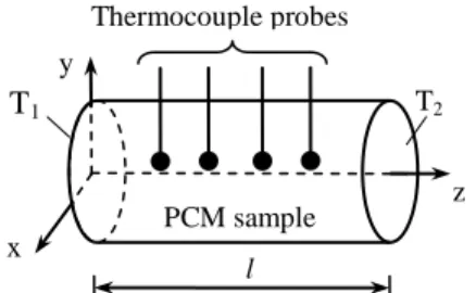
The proposed method consists of a cyclic cooling and heating of the PCM sample placed into a holder tube and a monitoring of the temperature field evolution inside the probed PCM using a set of thermocouples. Temperatures are applied on both sides of the tube and the PCM (T1 and T2). The experimental
setup of this measurement approach is schematically depicted in figure 1.
Figure 1. Schematic of the experimental arrangement x z y Thermocouple probes PCM sample l T2 T1
The amount of PCM is relatively small, while the sample holder design includes a variety of auxiliary elements (such as a set of temperature sensors and its mounting assemblies, a thermal expansion compensator tube, tubes to fill and remove the PCM samples etc.). The effect of these elements on the heat transfer is not negligible. It is clear that the calculation accuracy achievable using a simple one-dimensional approach (analytical or numerical) is not sufficient to get the right solution. Consequently, we need a computational tool that makes it possible to calculate more accurately the temperature fields in computational domains having a complex 3D geometry. Therefore in this work, we selected the well proven COMSOL Multiphysics® software package to implement the parameters estimation iterative procedure.
The practical implementation of the considered metrological task relates to solutions of two problems: direct (forward) and inverse. While the former deals with calculating the spatial and temporal temperature distribution into the PCM samples associated with selected parameter values, the latter consists in an estimation of the PCM parameter values from the measured temperature distribution.
The direct problem can be solved analytically or numerically using the heat transfer equation with the boundary and initial conditions as per the experimental setup configuration. The most common approach to inverse problem solving involves a so-called sensitivity analysis that addresses the impact of the variations of the PCM thermal parameters on the temperature field distribution and its temporal evolution in the sample [2].
2.1 Inverse Problem Formulation
The inverse problem pertains to define the PCM thermal parameters (such as the latent heat of fusion, the thermal conductivity, as well as the specific heat in solid and liquid states) from experimental measurements of the thermal response history.
The procedure to estimate the vector of parameters Y involves the minimization of the difference between the measured variation U of temperature with time at Np selected points of
the PCM sample and its theoretical values T, obtained by solving the direct problem [3]:
T
min Y U Y T U Y T Y (1)The nomenclature is summarized in table 1 (see Appendix). In matrix form, the necessary minimum condition of this functional can be written as follows:
Y
TY U
0ZT (2)
In this equation, the elements of the sensitivity coefficients matrix Z are the derivatives:
j k i k ij Y T Z (3)
These derivatives values can be calculated by solving the direct problem and they determine how the Yj thermal parameter affects the
temperature in the i-th selected points of the PCM sample at the k-th moment.
The solution of the inverse problem can be easily found using the so-called sensitivity coefficients iterative method [3]. This method involves the following algebraic set of equations:
T
1
1
T n n n Y Z U Y T Z Y Z Z (4), where Y(n) and Y(n-1) are respectively the vectors of parameters estimated in n-th and (n-1)-th iterative steps.
Therefore the solution of the inverse problem requires the knowledge of the sensitivity coefficients matrix. In this work, we calculate the elements of this matrix using numerical models implemented in the COMSOL Multiphysics® software.
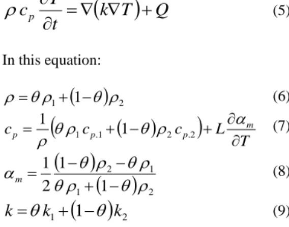
2.2 Heat Transfer Governing Equations The viscosity of most of the commercial low-melting temperature PCMs at temperatures close to the melting point is usually very large. In addition, in the implemented experimental setup, the length to diameter ratio of the tube is relatively high and the volume of PCM is relatively small. Accordingly, the heat transfer by convection can be supposed to be negligible. Thus we use a simplified approximation in the numerical models, in which the heat transfer in the PCM is dominated by conduction. The mathematical formulation of this problem involves the classic heat transfer equation, [4, 5]:
k
T
Q
t
T
c
p
(5) In this equation:
2 1 1
(6)
T L c c c m p p p
1 .1 1 2 .2 1 (7)
2 1 1 21
1
2
1
m (8)
2 11
k
k
k
(9)We invistigated independent and time-dependent Dirichlet boundary conditions. In the former case, the left and right vertical walls (figure 1) are kept at fixed temperatures:
Const
t
T
(
0
,
)
;T
(
l
,
t
)
Const
(10) , while the initial conditions were specified with a 4-th-order polynomial:
4 00
,
n n nz
a
z
T
(11)In the latter case, the boundary and initial conditions are:
t
T
t
T
(
0
,
)
1 ;T
(
l
,
t
)
T
2
t
(12) meltingT
Const
t
z
T
(
,
0
)
(13)In both cases, the lateral cylindrical wall was assumed to be thermally insulated:
0
n k T (14)
It is instructive to note that both of these approaches reveal a good agreement between the experiment and the results obtained.
3. Use of the COMSOL Multiphysics®
Software
The COMSOL Multiphysics® software package is used as a powerful computational tool to solve the direct problem, necessary to calculate the sensitivity coefficient matrix for the PCM thermal parameters, eq. (3), required to
perform the iterative procedure of the PCM parameters estimation, as noted above. We used the heat transfer module of the software to calculate and analyse the temperature field in the PCM sample, as well as its temporal variation, taking into account the 3D geometry of the experimental setup used for the PCM samples characterization.
The geometrical design of the PCM sample holder is depicted schematically in figure 2.
Figure 2. Sample holder geometry used in the COMSOL numerical model: 1- Plexiglas tube; 2- PCM sample; 3- holes for thermocouple probes In the numerical simulations, the values of the parameters for the materials used in the sample holder (Plexiglas, metals, etc.) were taken from the COMSOL Multiphysics® software built-in material library. Moreover a temperature interval of 0.5K has been considered around the phase change temperature of the PCM [5]. The procedure to estimate the parameters pertains to the temporal evolution of the temperature field. Accordingly, in our numerical simulations we use the time-dependent solver. A comparative analysis of experimental and numerical results reveals that, the most optimal mesh in terms of computation time is the “Normal Physical” one, suggested in the software.
4. Results and discussion
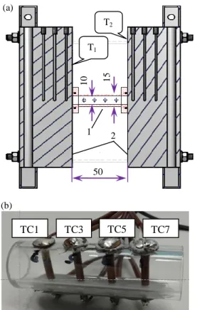
The first proof-of-concept prototype used in the experiment to characterize the PCM samples is shown in figure 3.
It is composed of a Plexiglas tube sample holder (1) filled with PCM sandwiched between the two aluminium blocks (2). The tube material is chosen to limit the conductive heat fluxes with the PCM and foam is placed all around it to insulate at best from the environment. The heat loss in the radial direction can then be supposed negligible.
2 1
The real-time temperature distribution measurement in the PCM sample is monitored by a set of four thermocouple probes (TC1, TC3, TC5 and TC7).
The temperatures of the blocks are controlled using a dedicated cooling-heating system developed by our research group (not shown in this figure).
Figure 3. Experimental setup: (a) measurement cell; (b) Plexiglas tube sample holder with a set of four thermocouple probes
Figure 4 depicts an example of the results obtained with the numerical simulations performed for the sample holder. In figure 4 a), a temperature field is shown at time 13700s. The corresponding solidification front is represented in figure 4 b).
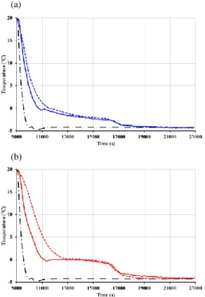
Besides, typical temperature plots were calculated with the numerical model and compared to the experimental curves as depicted in figure 5, for half of a cooling-heating cycle. The plot starts at 9000s when the cooling phase begins. The solidification at TC1 occurs a bit before 11000s while it begins around 13000s at TC3.
It should be noted that in the first study phase dedicated to the testing of the developed experimental setup, as well as to the estimation procedure abilities, we prefer to use the most common materials with well-known thermal properties, such as distillate water (PCM sample), Plexiglas, etc. The physical properties of the used materials are summarized in Table 2 (see Appendix). In addition, symmetric conditions are applied such that the boundary temperatures T1 and T2 are equal.
Figure 4. Example of the results obtained using the COMSOL numerical model: (a) temperature field distribution (°K) at t=13700s ; (b) solidification fronts at t=13700s
Figure 5 clearly demonstrates a good agreement between experimental data and numerical simulations results during the solidification. A disagreement between the model and the experiment is observed at the beginning of the test. It may be attributed most likely to instrumental errors in the measurement and inaccuracies in the current numerical model that does not take into account all physical effects. A better agreement between the numerical and the experimental results at the beginning of the 50 15 10 T1 T2 1 2 (a) (b) TC1 TC3 TC5 TC7 (a) (b)
cooling process could be obviously achieved after modelling the natural convection.
Figure 5. Example of the transient temperature curves of a PCM sample (here for distillate water) obtained for two thermocouple probes: (a) TC1 and (b) TC3. The solid lines represent experimental curves; the dashed lines denote calculated temperature curves, while the dot-dashed lines depict the temperature of the aluminium blocks (see figure 3).
Nevertheless, in practice, most cold storage systems operate at a relatively narrow temperature range around the PCM melting temperature, where the PCM viscosity is relatively large (see for example [6]). Within the experimental operating conditions of interest in this work, the contribution of natural convection is practically insignificant. Accordingly during the solidification, the developed numerical model is still accurate enough to use the sensitivity analysis procedure.
As mentioned above, for a given parameter, the sensitivity coefficient calculation involves two numerical solutions of the direct problem (Eqs. (5)-(14)): one with the base parameter value and the second with the parameter
perturbed. Thus in order to completely characterize a PCM sample, we need to perform at least 16 numerical simulations (there are 8 parameters to be estimated: kS, kL, cp,s, cp,L, λ, ρS,
ρL and Tm). In addition the sensitivity analysis
was also carried out for the tube in Plexiglas (ρ, cp, k). An example illustrating the sensitivity
coefficient calculation procedure is shown in figure 6. In this example, the perturbed value of the latent heat is set to 90% of the initial value. In our case the sensitivity coefficients calculated for the PCM thermal parameters reach the maximum values in the range from 16000s to 21000s. Thus, this part of the curves represents the optimal region to perform the estimation of the PCM thermal parameters.
Figure 6. Transient temperatures (a) calculated at the position of the TC3 thermocouple probe for the base (solid line) and perturbed (dashed line) values of the PCM latent heat; the resulting value of the sensitivity coefficient (b) calculated using the Eq. (3)
After the sensitivity coefficients matrix is generated, the procedure to estimate the parameters becomes a quite simple task. This procedure involves additional programming routines for solving Eq. (4), easy to implement (a)
(b)
(a)
with any available software including matrix computation tools (such as MATLAB®).
5. Conclusions
In this paper, we present an original and simple instrumental setup dedicated to the monitoring of the irreversible thermal effects in a PCM, induced by cyclic melting and freezing. The proposed metrological approach can be implemented with ease, although it requires an additional data processing procedure. In this work, we use the COMSOL Multiphysics® software to investigate the temperature history of the PCM sample, as well as its sensitivity to the variations of the PCM’s thermal parameters. An experimental setup involving this approach has been designed, assembled and tested. Some intermediate results have been reported and discussed. The experimental work related to the PCM characterization is currently under progress. The detailed description of the obtained experimental results will be presented in a near future.
6. References
1. H. Mehling, L.F. Cabeza, Heat and cold storage with PCM, An up to date introduction into basics and applications, Springer-Verlag Berlin Heidelberg, (2008).
2. Jingchao Xie et al., Comments on Thermal Physical Properties Testing Methods of Phase Change Materials, Advances in Mechanical Engineering, 2013, Article ID 695762 (2013). 3. A. Wawrzynek, M. Bartoszek, Inverse heat transfer analyses as a tool of material parameter estimation, Proceedings of conf. Thermo-physics 2006, Thermophysical Society, Bratislava, 03-19, (2006).
4. V. Alexiades, A. D. Solomon, Mathematical Modeling of Melting and Freezing Processes, CRC Press, (1992).
5. COMSOL 5.2, Heat Transfer Module User’s Guide.
6. J. Kestin et al, Viscosity of liquid water in the range -8°C to 150°C, Journal of Physical and Chemical Reference Data, 7/3, 941-948 (1978)
7. Acknowledgements
This research was performed with a financial support from the Walloon region, Belgium.
8. Appendix
Table 1: Nomenclature:
λ Latent heat of fusion, [J/kg] ρ Density, [kg/m3]
k Thermal conductivity, [W/m2K] cp,s Specific heat in solid state, [J/kg K]
cp,L Specific heat in liquid state, [J/kg K]
Tm Melting temperature, [K]
θ Liquid-solid fraction, [A.U.] T Temperature, [K]
t Time, [s] Q Heat, [J] m Mass, [kg]
U Matrix of the measured temperature values, [K]
T Matrix of the theoretical temperature values, [K]
Y Vector of the PCM thermal parameters
Table 2: Parameter values used in the numerical simulations
Parameter/Material Parameter value
Water / Ice cp=4202/2101 [J/(kg∙K)] k=0.56/2.3 [W/(m∙K)] ρ=1000/920 [kg/m3] λ=334 [kJ/kg] Tm=273.15 [K] Copper cp=385 [J/(kg∙K)] k=400 [W/(m∙K)] ρ= 8700 [kg/m3] Plexiglas cp=1460 [J/(kg∙K)] k=0.187 [W/(m∙K)] ρ= 1190 [kg/m3] Initial temperature