HAL Id: hal-02981422
https://hal.uca.fr/hal-02981422
Preprint submitted on 9 Nov 2020
HAL is a multi-disciplinary open access archive for the deposit and dissemination of sci-entific research documents, whether they are pub-lished or not. The documents may come from teaching and research institutions in France or abroad, or from public or private research centers.
L’archive ouverte pluridisciplinaire HAL, est destinée au dépôt et à la diffusion de documents scientifiques de niveau recherche, publiés ou non, émanant des établissements d’enseignement et de recherche français ou étrangers, des laboratoires publics ou privés.
Green Bond market vs. Carbon market in Europe : Two
different trajectories but some complementarities
Yves Rannou, Pascal Barneto, Mohamed Boutabba
To cite this version:
Yves Rannou, Pascal Barneto, Mohamed Boutabba. Green Bond market vs. Carbon market in Europe : Two different trajectories but some complementarities. In press. �hal-02981422�
Green Bond market vs. Carbon market in Europe:
Two different trajectories but some complementarities.
Yves Rannou
1Pascal Barneto
2Mohamed Amine Boutabba
3This version: June 30, 2020
Abstract
Europe has been the first continent to create a large-scale carbon market to reduce the level of carbon emissions and to create a green bond market to finance the transition to low-carbon economies concomitantly.
In this chapter, we study the respective roles of these instruments, their price trajectories, their interaction and their potential complementarities over a six-year period (2014-2019).
We enrich the literature on environmental markets in several respects. First, significant short-run and long-run persistence of shocks to the conditional correlation between the European carbon and the European Green bond markets are reported. Second, we detect bi-directional shock transmission effects between those markets but no significant spillover effects. Taken together, these results suggest that a green bond issued in Europe may be used to hedge against the carbon price risk.
KEYWORDS: Green Bond, European Allowance, Spillover effects, Asset Complementarity
JELCODES : G11, G12, G13, Q56
1 Yves Rannou. Groupe ESC Clermont – CleRMa, 4 boulevard Trudaine, 63000 Clermont-Ferrand, France.
Email : yves.rannou@esc-clermont.fr.
2 Pascal Barneto. Institut d’Administration des Entreprises (IAE) de Bordeaux – IRGO, 35 avenue Abadie, CS
51412, 33072 Bordeaux cédex, France. Email : pascal.barneto@u-bordeaux.fr.
I. Introduction
Creating a green and low-carbon economy represents a global market opportunity for all investors, financial institutions and firms. In Europe, the European Green Deal's Investment Plan, unveiled on January 2020 by Ursula von der Leyen, aims to mobilise €1 trillion of
investments in the next decade at least. Two months after, the European Commission (EC
hereafter) presented its proposal for the European Climate Law, part of the European Green
Deal, to serve EC’s vision to be climate neutral by 2050. With this European Green Deal
Package, Europe remains to be at the forefront of climate change mitigation and adaptation. Europe has been the first (and the only) continent to promote the use of carbon markets to reduce the level of carbon emissions and of green bond market to finance the transition to low-carbon economies quasi simultaneously. The European Union Emission Trading Scheme (EU ETS hereafter) that results in the European carbon market was used to achieve both greater environmental effectiveness and lower overall cost of mitigation. The Stern–Stiglitz High-Level Commission on Carbon Prices, while recognizing that “A well-designed carbon price is an indispensable part of a strategy for reducing emissions in an efficient way,” called in 2017 for “explicit price trajectories.” Carbon pricing provides mitigation incentives and indirectly reduces the vulnerability of the economy to climate change. Since a breakthrough in fiscal policy is unlikely, additional financing resources like green bonds, are necessary.
Issuing green bonds is a an other solution for financing climate change mitigation, adaptation that has been implemented in Europe. Since the first green bond issued by the European Investment Bank (EIB) in 2007, the European Green bond market has grown quickly and is now valued at 118.6 billion dollars of issuances in 2019 (CBI, 2020).
Green bonds are used for mitigation issues to a large extent but also for adaptation to climate change impacts. However, some studies have pointed out that they may be more expensive than conventional bonds raising the cost of debt (e.g., Zerbib, 2019). Bachelet et al. (2019) found that the act of certifying a green bond reduces its yield so issuers can reduce de facto debt costs for green investments. Another reason to issue green bonds is the diversification of the investor base (Thang and Zhang, 2018) and its communications role. Many corporates have made long-term climate commitments. Issuing green bonds can help signal (implicit) carbon pricing. Unlike carbon pricing, green bonds do not provide the needed marginal incentives for corporates to optimally factor carbon costs into their decision making. Overall, the contributions of these instruments seem to be negligible for containing climate change.
This chapter examines the roles of these instruments, their price trajectories, their interaction and their potential complementarities over a six-year period (2014-2019).
While carbon markets and green bonds are jointly implemented, they interact in two ways at least. First, holders of green bonds may be interested in tightening ETS caps. An ETS sets a cap on emissions, and emissions leakage can occur if green bonds finance climate change mitigation projects for industries covered by the ETS. Mitigation effects obtained via green bonds decrease the scarcity of EUAs under the cap, reducing the carbon price. To prevent this decrease, the emissions cap should be tightened when green bonds are introduced. A second interaction effect between green bonds and carbon prices works through price volatility. Green investment projects can more easily attract green bond financing if returns on investment are less volatile. As their returns depend on carbon prices, a more stable carbon price also generates a more stable return on investment and greater demand for green bonds simultaneously.
The financial engineering techniques operate at two levels for both carbon assets (EUAs) and green bonds. In terms of product innovation, green bonds can be issued with specific attributes (fixed/variable coupons, callable features,…) whereas EUAs can be traded via spot contracts or a large range of derivatives contracts (futures, options, strips of futures, swaps). In terms of risk management, green bonds and EUAs are volatile assets that require accurate estimation of their volatility (risk) so investors can adapt their hedging policies in consequence. In the literature, few attempts have already been made to model portfolio and/or risk strategies including a carbon asset and a green bond. For instance, Rannou (2019) builds a model of two assets traded in a continuous double auction market: (i) a EUA traded at the prevailing price and (ii) a green bond that pays out a fixed payoff at the end of maturity.
However, to the best of our knowledge, no papers has yet compared the price dynamics of the European Green Bond market and that of the European carbon market notably during the Phase III of EU ETS (2013-2019), where the EUA (auctioned) has an initial price. The difficulty here is that the carbon market and the green bond market in Europe are not directly comparable through their primary or their secondary market. Regarding the primary market, the issuance of EUAs that are auctioned is strictly managed by the EC while the issuance of green bonds is only subjected to the approval of stock exchanges provided that they are certified or labelled (Bachelet et al. 2019). Regarding the secondary market, the European carbon market enjoys a liquid secondary market (Medina et al., 2013; Stefan and Wellenreuther, (2020) in contrast to the European Green Bond that suffers from an illiquid secondary market (Zerbib, 2019).
To remedy these difficulties, we proceed in two steps.
First, we employ the European green bond and EUA carbon indices rather than using prices of stock exchanges. Second, we develop a VAR BEKK GARCH model, particularly adequate to capture volatility shocks as well as volatility spillover effects between European carbon market and the European Green bond (GB hereafter) market and vice versa.
Three important results emerge from our empirical work. First, we observe significant short-run and long-run persistence of shocks to the dynamic conditional correlation between EUA and GB (EUR) markets but not between EUA and GB Global markets. Second, the dynamic conditional correlation coefficient between EUA and GB Euro markets is low fluctuating in the range 0.01–0.12 from 2014 to 2018. Since the beginning of 2019, it becomes slightly negative. This result can be explained by the good carbon market performance in 2019 due to the drop in emissions of electricity producers and the use of the Market Stability Reserve, a sort of central allowance bank, intended to reduce too abundant supply of EUAs in order to maintain EUA prices at a certain level. Third, we detect bi-directional shock transmission effects between EUA and GB (EUR) while a one-way positive volatility spillover effect from GB (Global) to EUA is reported.
Taken together, these results suggest that the green bond instrument issued in Europe may be used to hedge against the EUA carbon price risk. This finding is important for investors and for fund managers that may invest in green bonds and in EUA futures to create a portfolio of environmental assets. Henceforth, these financial assets can be considered as complementary.
The rest of this chapter is organised as follows. In Section 2, the role and the evolution of the European carbon market are presented. Section 3 reviews the role and the development of the European Green Bond market. Section 4 analyses the interaction of the price dynamics of both the European carbon market and the European Green Bond Market. Section 5 concludes.
II. The Carbon market in Europe
« Carbon trading is set to become the world's largest commodity market. The world emits 35 billion tons; priced at $20; that’s $700 billion. Put a 10-20 multiple […] you’re talking about $10 trillion at maturity. » R. Sandor (2010), founder of the European Climate Exchange (ECX) 2.1. Economic concept of the carbon market (EU ETS)
There are two ways to establish a carbon price. First, a country can levy a tax on carbon
content i.e. the CO2 emissions caused by its production. Second, a government or a
supranational authority can establish a system in which the aggregate level of emissions covered by the quotas is set equal to the desired level of total emissions and quotas are tradable – an ETS (e.g., the EU-ETS in Europe). A carbon tax gives certainty over the price of carbon whereas an ETS can lead to high price volatility, because the inelasticity of the supply of permits combines with inelastic demand for permits in the short run. But the volatility is reduced by allowing ‘banking and borrowing’ of quotas across time periods and/or by introducing hybrid schemes in which sharp price movements trigger a change in the authorities’
supply of quotas (e.g., Market Stability Reserve) (Monast, 2010).4 More importantly, both a
carbon tax and an ETS can raise revenue as long as, in the latter case, the quotas are auctioned. 2.2. Current framework of the European carbon market
Issued by the Directive 2003/87/EC, the EU-ETS is a cap and trade scheme that controls
the CO2 emissions of more than 12,000 regulated installations, that mainly come from industrial
and power sectors, and from aviation since 2012 (European Commission, 2013). The principles of the carbon market as a cap-and-trade scheme are twice. First, a global cap of emissions is
set; an equivalent number of EUAs (i.e. quotas to emit 1 tCO2 equivalent) – is issued and
allocated to the regulated installations. An installation must reach compliance by surrendering the number of EUAs equal to its verified emissions. This is the cap. The level of emissions reductions essentially depends on the cap and not on the trade: the incentives to reduce emissions depend on the more or less restricted allocation, since emissions cannot exceed the number of EUAs issued. Second, polluting firms are required to purchase EUAs for each ton of carbon dioxide missing by trading them on secondary spot or futures markets. In Phase I (2005–2007) and Phase II (2008-2012) of EU ETS, nearly all EUAs were given away for free. In Phase III (2013-2020), the EU objective of 21% reduction of GHGs in 2020 relative to 1990
4 In the carbon market, in the absence of a “safety valve”, a rocketing carbon price could seriously damage the
levels imposes the 27 EU Member States to introduces gradually auction sales for EUA so that free allotment has been reduced significantly. From 2013, the shifts towards an auction-based allocation process should create a larger primary market for EUAs, with more attention paid to the long-term by investors. This also raises the importance of futures markets as an effective tool to hedge against unexpected changes in the carbon price. In fact, it is widely accepted that the European carbon market encounters a recurrent problem of low and volatile prices since the beginning of EU ETS. During Phase I (2005-2007), the EUA price fell because of a strong over-allocation of EUAs. During Phase II (2008-2012), the EUA market experienced a significant price drop because of the economic crisis that impacted industrial production, and therefore the level of carbon emissions. At the beginning of Phase III, in 2013, the EUA price decreased below €5 that remains too low to favour the switching to low-carbon technologies.
Medina and Pardo (2013) document the existence of heavy tails, volatility clustering, asymmetric volatility in EUAs returns. They also provide evidence of negative asymmetry, positive correlation with stock indexes and higher volatility levels, typical of financial assets, and the existence of inflation hedge and positive correlation with bonds, characteristic of commodity futures. In this way, EUAs may be viewed as a new asset class. Other studies have highlighted the influence of two other attributes of the EUA market making it specific:
Information asymmetry. In the financial market, issuers are responsible for the information released to the public, under the supervision of the regulator whose task it is to design and check the rules so that all investors have transparent information as to the risks involved. In the carbon market, the public authority is the single issuer of EUAs, transactions of which are tracked by the registries network. Thus, the registries could provide the market with exhaustive information on spot trades, almost in real time. This information remains “private” because it cannot be released to the public for five years. Such private information is held by EU ETS compliant (“informed”) firms. This information is closely monitored by market participants. In addition, Rannou (2019) identifies a second important source of information asymmetry namely adverse selection costs that uninformed traders bear when they trade EUAs with informed counterparty traders through an exchange based platform (i.e. limit order book).
Risk Aversion. Chevallier et al. (2009) detected a lower volatility after that the amount of verified emissions corresponding to the 2006 compliance period was disclosed to the public. They also estimate that risk aversion is higher on the EUA market than on equity markets in Phase I and Phase II. It is directly related to the uncertainty around the compliance events and political decisions related to the future of EU ETS (e.g., level of the emission cap in next Phase).
2.3. Market segments in the EU ETS
As is the case with stock or commodity markets, we can distinguish the EUA primary market (issuance of new EUAs that are auctioned in Phase III) from the EUA secondary market that offers EUA spot or futures contracts for trading.
Primary market. From a theoretical point of view, the EU ETS is a compliance market, where regulated installations seeking to cover their emissions can purchase an equivalent number of EUAs on a primary market. In Phase III, the primary (auction) market only takes place at the EEX exchange (except for UK where auction occurs on the ICE ECX exchange).
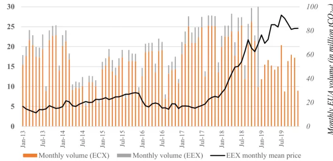
Figure 1 plots the evolution of EUA prices traded on the primary market of EEX along almost the entire Phase III (2013-Dec 2019). We observe that the EUA price has increased fivefold in spite of a slight increase of EUAs issued. This significantly higher price should clearly encourage power and industrial companies to switch to low-carbon technologies. Figure 1. Price evolution and volume of EUAs issued on the primary market (2013-2019)
Secondary market. In practice, the EUA market is also a financial market, to the extent that EUA derivatives (i.e. futures and options) are traded by market participants searching for hedging or speculating. Interestingly, Lucia et al. (2015) found that the influence of speculators in the EUA futures market are higher than this of hedgers after the disclosure of verified emissions to the public in May. Spot contracts and options on EUA futures are also available for sale representing less than 10% each of the EUA trading volume recorded on exchanges (Mizrach, 2012). The European Climate Exchange (ECX) has dominated the trading of EUA futures that represents 80% of EUA trading volume in Phase II (Rannou and Barneto, 2016).
0 20 40 60 80 100 0 5 10 15 20 25 30 Ja n-13 Ju l-13 Ja n-14 Ju l-14 Ja n-15 Ju l-15 Ja n-16 Ju l-16 Ja n-17 Ju l-17 Ja n-18 Ju l-18 Ja n-19 Ju l-19
Monthly volume (ECX) Monthly volume (EEX) EEX monthly mean price
E E X m on th ly p ri ce o f E U A = 1t C O2e q M on th ly E U A v ol um e (i n m ill io n tC O2e q )
Accordingly, an important strand of research has investigated the price discovery function of EUA futures markets. Rittler (2012) shows that the carbon price discovery mainly occurs in this market. Rannou and Barneto (2016) find that flows of private information are controlled and lagged by informed traders by executing large trades on OTC market, while flows of public information are constrained on exchanges encouraging mimetic (speculative) trading from uninformed traders that fuel higher price volatility (risk). In Phase II, Boutabba (2009) shows that the ICE-ECX is more influential in the information transmission process even if prices traded on European Energy Exchange (EEX) affect those of ICE-ECX. In the current Phase III, the ICE-ECX in London and the EEX in Leipzig, are the two most active exchanges where EUA futures with similar contract specifications are traded (Stefan and Wellenreuther, 2020).
2.4. Market participants
From Table 1, we can notice that power and industrial companies covered by EU ETS account for 29% of the ICE-ECX market participants. Neuhoff et al. (2012) identify and characterise three main trading strategies that they could follow:
- Hedging by rollover EUA (December) futures contracts to minimise trading costs; - Making arbitrage between different maturities of EUA futures contracts (strip futures)
on ECX in priority because it is the most liquid platform.
- Speculating by contracting or maintaining open positions (Lucia et al. 2013). Because speculative buyers of EUAs carry more risk, they require higher returns.
Institutional investors (e.g. fund managers, portfolio managers, insurance companies) represent 20% of ICE-ECX members, much less than in stock and bond markets. They may arbitrage the spot/futures basis or hedge their exposure to (spot) carbon price volatility by trading EUA futures. Also, they may have followed speculation strategies like momentum strategies to continue a given price direction and make profits (Rannou and Barneto, 2016). Also, they may have pursued diversification strategies by investing in carbon in a portfolio together with other assets including energy, stock, ETFs, bonds, or invest in EUAs as part of a larger “green” portfolio including green bonds (De Croce et al., 2011).
20% of ICE-ECX members are (investment) banks. They provide a wide range of services including order and trade execution, clearing of exchange-based or OTC trades but also research on carbon markets (fundamental analysis and chart analysis to determine price trends). They could also engage in arbitrage and in hedging carbon strategies by trading EUA futures.
Brokers represent 16% of ECX members. According to Mizrach (2012), nine major brokers who are also members of the London Energy Brokers Association except MF Global
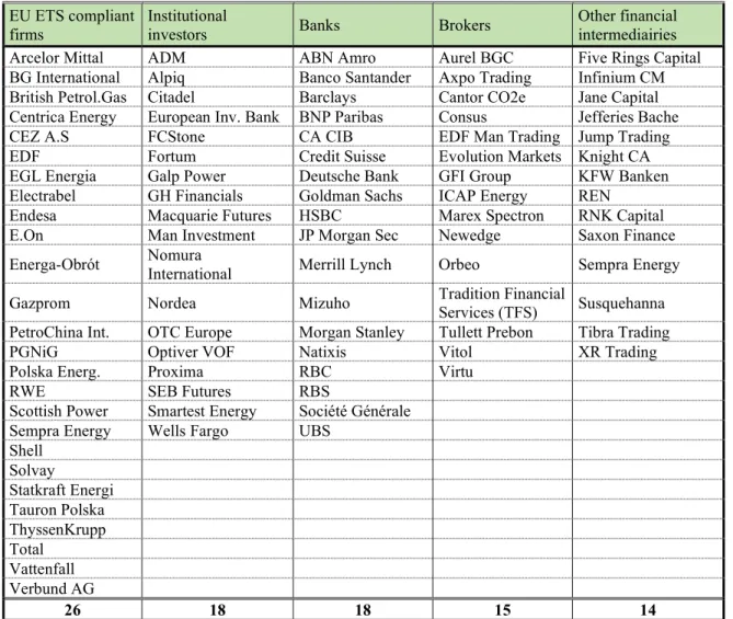
(Aurel BGC; CantorCO2e; Evolution Markets; GFI Group; ICAP; Marex Spectron; TFS; and Tullett Prebon) are really active on the EUA secondary market of ICE-ECX. They benefit from invaluable information related to the order flow (i.e. price and volume of orders) of their clients thanks to their dual role (principal-agent). Finally, the remaining 15% of ICE-ECX members are financial intermediaries (other than brokers). They have either market making activity (e.g. Five Ring Capital, Jump Trading) and/or behave as day traders (arbitrage and speculation). Table 1. Market participants trading EUA spot and futures contract on ICE-ECX (2013-2019)
EU ETS compliant
firms Institutional investors Banks Brokers Other financial intermediairies Arcelor Mittal ADM ABN Amro Aurel BGC Five Rings Capital BG International Alpiq Banco Santander Axpo Trading Infinium CM British Petrol.Gas Citadel Barclays Cantor CO2e Jane Capital Centrica Energy European Inv. Bank BNP Paribas Consus Jefferies Bache CEZ A.S FCStone CA CIB EDF Man Trading Jump Trading EDF Fortum Credit Suisse Evolution Markets Knight CA EGL Energia Galp Power Deutsche Bank GFI Group KFW Banken Electrabel GH Financials Goldman Sachs ICAP Energy REN
Endesa Macquarie Futures HSBC Marex Spectron RNK Capital E.On Man Investment JP Morgan Sec Newedge Saxon Finance Energa-Obrót Nomura International Merrill Lynch Orbeo Sempra Energy Gazprom Nordea Mizuho Tradition Financial Services (TFS) Susquehanna PetroChina Int. OTC Europe Morgan Stanley Tullett Prebon Tibra Trading
PGNiG Optiver VOF Natixis Vitol XR Trading
Polska Energ. Proxima RBC Virtu
RWE SEB Futures RBS
Scottish Power Smartest Energy Société Générale Sempra Energy Wells Fargo UBS
Shell Solvay Statkraft Energi Tauron Polska ThyssenKrupp Total Vattenfall Verbund AG 26 18 18 15 14
III. The green bond market in Europe
« I do think there are a number of investors who would love to have sovereign green bonds in their portfolios. What I would like to see is what are they going to pay me for it? » Sir Robert Stheeman, Head of the UK Debt Management Office 3.1. Green bond definition and label
Green bonds are among the most popular debt instrument used in which the proceeds will be exclusively and formally applied to projects or activities that promote climate or other environmental sustainability purposes through their use of proceeds. Also called climate
bonds5, by purchasing these bonds, investors lend a fixed amount of capital to the issuer which
repays the capital (principal) and accrued interest (coupon) over a set period of time. The difference with a conventional bond lies in the channeling of the investments to projects that generate environmental benefits, for instance in renewable energy, energy efficiency, sustainable waste management, sustainable land use (forestry and agriculture), biodiversity conservation, clean transportation and clean water. It is a common practice for issuers to rely on independent experts to validate the environmental quality of the proposed projects.
On the one hand, benefits for green bonds issuers include reputational gains (Thang and Zhang, 2018) as well as upgraded risk management processes due to their commitments to better inform on their exposure to climate change. On the other hand, the main benefit for bondholders, especially long-term and responsible investors is related to the opportunity provided to diversify their portfolios with green bonds issued in respect to their correspondence to ESG (Environmental, Social, Governance) criteria.
At present, the Green Bond Principles (GBP) is the most commonly referred basis for ensuring that bonds wishing to claim to be ‘green’ can do so by compliance with those principles. These are voluntary guidelines elaborated by key market participants under the coordination of the International Capital Markets Association (ICMA) acting as secretariat. The GBP covers four key mandatory principles: (i) the description of the use of proceeds which need to finance assets and projects with positive environmental impacts, (ii) the requirement of a clear process for the selection of projects and (iii) a description how the funds are allocated or tracked, (iv) reporting on the use of proceeds with, if possible, information on the environmental impact of the projects. Accordingly, the green credentials of green bonds can be structured into four categories. Bonds related to tax revenues (use-of-proceeds revenue bonds)
5 Climate bonds are a type of green bond which specifically are supposed to address climate change problems,
represent a large segment of Green Bond market. Green project bonds and green securitized bonds constitute relatively small niche markets that have recently attracted more attention, with the first securitized bond being issued in the Eurozone by Berlin Hyp in 2015.
The EU is leading that effort to formalize regulations. The first set of rules, called the Green Bond Standard, building on the GBP, was planned for 2020. A second — a 414-page taxonomy that will set definitions for sustainable activities or projects — was expected to be in place by 2022. These rules ultimately should eliminate any uncertainty about how proceeds can be used and how issuers should manage the green bond designation process.
3.2. Current framework of the EU green bond market
The origin of the green bond market is dated to 2007 when the EIB issues its « Climate Awareness Bond » focused on renewable energy and energy efficiency. From 2008 to 2013, green bond issuance is mainly dominated by Sub-sovereign, Supranational and Development
Agency (SSA or MDBs)6. Various corporates such as Bank of America, EDF, Vasakronan,
Toyota7 as well as municipalities and local governments such as Ile de France (Paris) and
Gothenburg (Sweden) regions have more recently joined the market, annual issuance of green bonds in Europe has nearly quadrupled from USD 11 billion in 2013 to USD 47.8 billion in 2015 with issuance in 14 from the G20 countries. This expansion continues in 2016 with an amount of USD 54.1 billion issuance estimates at the end of September. As a result, the outstanding amount of Green bonds issued has totalled USD 694 billion, of which USD 118 billion are due to labelled green bonds and USD 576 billion of unlabelled green bonds, as
reported in July 2016 (CBI/HSBC, 2016)8. European market continues to dominate global
issuance by reaching USD 116 billion in 2019, which accounted for 45% of global issuance. KfW, the German state-owned development bank and the Dutch State Treasury Agency (DSTA) are ranked as the second and the third largest global issuers in 2019, respectively.
6 In 2008, the World Bank (International Bank for Reconstruction and Development or –IBRD–) began its
marketing of green bonds with approximately a USD 440 million in response to specific demand from Scandinavian pension funds seeking to support climate-focused projects. Then, Multilateral Development Banks (MDBs) as the European Bank for Reconstruction and Development (EBRD) and the International Finance Cooperation have been key players in developing the global green bond market and helping it to become a mainstream capital market (European commission, 2016). SSA provided critical leadership by priming the market with low risk issuance and educating investors.
7 Toyota’s 2014 sale of securities with proceeds used for investment in electric vehicles and hybrids
8 Labelled green bonds are bonds that earmark proceeds for climate or environmental projects and have been
labelled as « green » by the issuer, while unlabelled green bonds refers to bonds whose proceeds are used to finance environmentally friendly projects, but do not yet carry the green label yet (CBI/HSBC, 2016).
3.3. Market segments and liquidity
As for the European carbon market, two complementary markets of green bonds in Europe can be distinguished: the primary (issuance) market and the secondary market.
Primary market. It is the marketplace where issuers offer their bonds to investors. According to CBI (2019), green bonds experienced good demand in the primary market, during the first semester of 2019, with larger book cover and spread compression than vanilla equivalents on
average. They have built yield curves on the issue date of a selected sample of green bonds to
determine whether there was a new issue premium called a “greenium” or the absence of one. The report of CBI (2019) conclude that this new issue premium paid by investors is unlikely.
Secondary market. It can be characterized as the trade of already issued green bonds. Stock exchanges play an important role in the secondary market to increase green bond visibility and promote transparency and market integrity. In 2007, the Luxembourg Stock Exchange became the first stock exchange to list a Green bond following the launch of the European Investment Bank’s “Climate Awareness” bond. Until now on, this platform leads the European green bond market in listing 170 Green bonds from over 40 different issuers with a collective value of $45bn. In 2019, USD 167 billion (€150 billion) worth of green bonds were listed on various stock exchanges, representing 65% of the total green bonds issued worldwide. Green bonds issued on the over-the-counter (OTC) markets account for 16% in 2019 while 19% were not listed or for which information was not available (CBI, 2020).
In spite of the rapid growth in green bond issuance over the past few years, the supply of green bonds may be insufficient due to a lack of fiscal incentive for green investment (Zerbib, 2019), and a missing global classification system for green bonds in relation to the widely used market-based best practices like the Green Bonds Principles. However, green bonds may in some cases be more attractive on the secondary market than conventional bonds. According to the fund manager Mirova (2018), the liquidity of the European green bond market may be considered satisfactory. Thus, investors are able to actively manage portfolios and take profit from arbitrage opportunities. Febi et al. (2018) find that green bonds traded on the two largest dedicated European market platforms namely the Luxembourg Green Exchange and London Stock Exchange are, on average, more liquid than conventional bonds, over the period 2014– 2016. In particular, the two employed liquidity measures: the LOT liquidity and the bid-ask spread are positively related to the yield spread. However, their results suggest that the influence of liquidity risk for green bonds on yield spread vanishes over time, which indicates that the European Green Bond market mature.
3.4. Market players
Six main categories of market players are active in the green bond market and interact: issuers, underwriters, external reviewers, intermediaries, index providers, and investors.
The issuers are the borrowers of the money and define the credit risk of the bond. In 2019, the largest issuers are non-financial corporates (27% of cumulative issuance) followed by Government-backed entities (22%), Financial institutions (21%), sovereigns (17,5%), Dvelopment bank (9,5%) and local government (1,5%) and sovereigns.
The underwriters manage the issuance process of the bond to the public. They work closely with the issuers to determine the bond-offering price at which the underwriters purchase the green bond from the issuer and sell them to investors. In 2019, some of the largest underwriters in terms of volume were Credit Agricole CIB, HSBC, SEB, BNP Paribas, Barclays, Societé Générale, Deutsche Bank, Natixis, Santander and ING.
Institutional investors are typically insurance companies and pension funds prefer investing in green bonds with maturity between 8 and 12 years. They follow buy and hold strategies in order to minimize trading costs in a context of a very illiquid secondary market.
External reviewers confirm alignment with specific guidelines or standards. They are specialised consultants, verifiers, certifiers, and rating agencies.
Other (financial) intermediaries include brokers, market makers or liquidity providers. Index providers track the green bond market performance by focusing on bonds where proceeds finance environmental projects. The Bloomberg Barclays MSCI Euro Green Bond Index is the dedicated index that tracks the performance of the green bonds issued in Europe.
IV. Interaction between European carbon and green bond markets
4.1. Data set description
Our empirical work focuses on the dynamic correlation and risk transmission between the Green Bond market and the carbon market in Europe. We use the S&P GSCI Carbon Emission Allowances (EUA) index (Total Return index) and the Bloomberg Barclays MSCI Euro Green Bond Index (Total Return Index Value Hedge). The former (EUA, hereafter) reflects the performance of European Union Allowance (EUA) Futures and calculated in Euro (EUR). The latter (GB (EUR), hereafter) is a market value-weighted index designed to measure the performance of green-labeled bonds issued in Europe. We also use the Bloomberg Barclays MSCI Global Green Bond Index (Total Return Index Value Hedge (GB (Global), hereafter) in order to assess volatility interaction between EUA market and global green bond market.
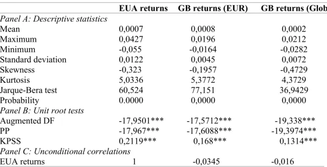
From January 10, 2014 to February 14, 2020, the sample contains 315 weekly observations. The logarithmic returns are used in this paper to depict the market volatility. Table 2 presents the summary statistics of EUA and GB returns.
Table 2. Summary statistics of EUA and GB returns.
EUA returns GB returns (EUR) GB returns (Global)
Panel A: Descriptive statistics Mean Maximum Minimum Standard deviation Skewness Kurtosis Jarque-Bera test Probability
Panel B: Unit root tests Augmented DF PP KPSS 0,0007 0,0427 -0,055 0,0122 -0,323 5,0336 60,524 0.0000 -17,9501*** -17,967*** 0,2119*** 0,0008 0,0196 -0,0164 0,0045 -0,1957 5,3772 77,151 0,0000 -17,5712*** -17,6088*** 0,168*** 0,0002 0,0212 -0,0282 0,0072 -0,4729 4,3729 36,9429 0,0000 -19,338*** -19,3974*** 0,1314*** Panel C: Unconditional correlations
EUA returns 1 -0,0345 -0,016
Note: Unit root tests (constant model) are performed on levels. The 1% critical values are −3.4507, −3.4507 and 0,739 for the Augmented DF, PP and KPSS tests, respectively.
*** denote statistical significance at the 1% level.
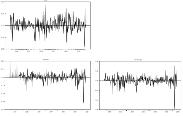
Broadly speaking, the returns of EUA and GB (EUR and Global) indexes vary over time (see Figure 2) and behaved in an opposite manner on the whole.
Moreover, Figure 2 depicts that the derived EUA and GB returns have significant volatility agglomeration characteristics. According to the mean or the standard deviation of each return series (Table 2), we can see that the volatility of EAU returns appears more significant than that of Green bonds. All the skewness coefficients are not equal to zero and all the kurtosis coefficients are above three, which indicate that EUA and GB returns series here all follow the fat-tailed non-normal distribution. All time series do not satisfy the normality assumption as supported by the Jarque-Bera test. Besides, the Augmented Dickey-Fuller (ADF), Kwiatkowski-Phillips-Schmidt-Shin (KPSS and Phillips-Perron (PP) tests are employed in this paper, and the results suggest that the three returns series are all stationary at the 1% significance level. The correlation values between EUA returns and the green bond returns low and negative illustrating the benefits of diversification in the short. The highest correlation is between EUA returns and GB (EUR) returns.
Figure 2. Evolution of weekly prices of Carbon and Green Bond indices (2014-2020)
Figure 3. Evolution of weekly returns of Carbon and Green Bond indices (2014-2020)
4.2. Methodology
The VAR model has been used to capture the linear interdependencies among multiple time series. In the current study, the VAR model is used to investigate the conditional mean, which provides the foundation for further volatility spillover research.
This bivariate VAR model for the EUA and green bond indexes is written as follows:
𝑟 = 𝑢 + ∑ 𝑎 𝑟 + ∑ 𝑏 𝑟 + 𝜀 (1)
𝑟 = 𝑢 + ∑ 𝑎 𝑟 + ∑ 𝑏 𝑟 + 𝜀 (2)
Where : 𝑟 and 𝑟 are the logarithmic returns of EUA and GB indexes at time t, respectively, while 𝑢 and 𝑢 are their respective conditional mean series. Lag orders are m and n with maximum lag values being M and N, respectively. Mean spillover coefficients 𝑎 and 𝑎 are for their own market and 𝑏 and 𝑏 are for across market. The residuals of Eq.(1) and Eq.(2) are respectively 𝜀 and 𝜀 .
Then, we apply the dynamic conditional correlation generalized autoregressive conditional heteroskedasticity (DCC-GARCH) model (Engle, 2002) to investigate the time-varying correlations between EUA and GB returns. The major advantage of the DCC-GARCH model is to examine time-varying market volatility spillover effects and possible changes in conditional correlation over time, implying dynamic portfolio behaviors in response to cross-market news. The DCC model is estimated in two steps: (1) we estimate a series of univariate GARCH parameters; (2) we assess their correlation estimations that vary over time.
Thus, the conditional covariance matrix can be decomposed as follows:
𝐻 = 𝐷 𝑅 𝐷 (3)
Where : 𝐷 = 𝑑𝑖𝑎𝑔 ℎ, is a 2 2 matrix containing the time-varying standard deviations
from the univariate GARCH model, and where 𝑅 = 𝜌 , (𝑖, 𝑗 = 1,2) is the 2 2 matrix
comprising the conditional correlations.
The generalized autoregressive conditional heteroskedasticity (GARCH) model captures two important market features: time-varying variance and leptokurtic distribution.
The standard deviations in Dt are presented by the following GARCH (1, 1) process:
ℎ = 𝛾 + ∑ 𝛼 𝜀, + ∑ 𝛽 ℎ, , 𝑖 = 1,2 (4)
Where : 𝜀 follows an independently and identically standard normal distribution with mean 0
and variance of 1, and i , i are the coefficients of the GARCH and ARCH terms. The
The conditional correlation matrix Rt is defined as follows :
𝑅 = 𝑄∗ 𝑄 𝑄∗ with : (6a)
𝑄 = (1 − ∑ 𝜃 − ∑ 𝜃 )𝑄 + ∑ 𝜃 (𝜀 − 𝑘𝜀 ) + ∑ 𝑄 (6b)
Where : 𝑄is the unconditional variance-covariance matrix from the model estimated in Eq.(4),
and 𝑄∗is a 2 2 matrix containing the square root of the diagonal elements of 𝑄 .
The dynamic conditional correlations are then given by:
𝜌 , =𝑞 ,
𝑞 , 𝑞 , (i,j = 1,2) (7)
Finally, we perform the BEKK model of Engle and Kroner (1995) which permits the interaction of the conditional variances and covariances of several time series. It therefore allows us to identify volatility transmission effects.
The conditional covariance matrix of the BEKK model, Ht , is expressed as follows:
𝐻 = 𝑊 𝑊 + 𝐴 𝜀 𝜀 𝐴 + 𝐵′𝐻 𝐵 with : 𝐶 = 𝑐 0 𝑐 𝑐 , 𝐴 = 𝑎 𝑎 𝑎 𝑎 , 𝐵 = 𝑏 𝑏 𝑏 𝑏 (8)
Where : C is a 2 2 lower triangular matrix of constants and C’ is its transposed matrix. 𝑎
and 𝑏 capture shocks and volatility spillover from EUA market to GB market. 𝑎 and 𝑏 capture shocks and volatility spillover from GB market to EUA market. 𝑎 and 𝑏 capture the impact of past shocks of EUA market and EUA on their own current volatility, respectively; and 𝑏 and 𝑏 capture the impact of past volatility of EUA and GB markets on their own current volatility, respectively.
4.3. Empirical results 4.3.1. Dynamic correlations
As stated above, the coefficients of the VAR-DCC-GARCH (1,1) model are estimated in two steps: the first step is to estimate the VAR model, while the second step is to evaluate the conditional correlation on the basis of residual errors estimations from the VAR model.
Table 2 shows the estimated coefficients of VAR-DDC-GARCH (1,1) with maximum likelihood (BFGS) and correlation targeting estimation between the return of EUA and GB indexes and the findings are shown as follows.
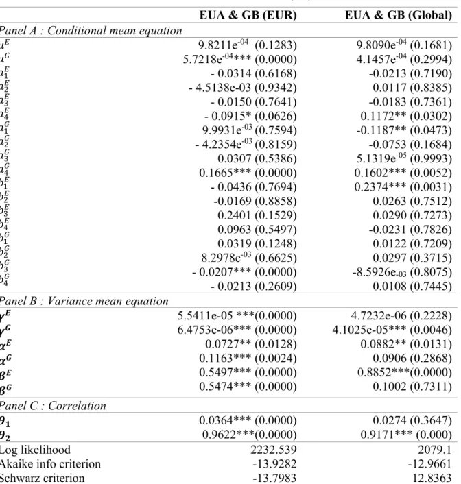
First, we observe significant short-run persistence of shocks to the dynamic conditional correlation between EUA and GB (EUR) markets as well, while it is not significant between EUA and GB (Global) markets. The finding provides some evidence of short-run predictability in the correlation changes between EUA and GB (EUR) market returns. Second, we document
significant long-run persistence of shocks to the dynamic conditional correlation between EUA market and GB (EUR) and GB (Global) markets.
Table 3shows that all the values of b are statistically significant and close to one, which
indicates that the long-run persistence of shocks is quite important for the long-run change prediction on the dynamic conditional correlation in the two cases.
Table 3. Estimated coefficients of the VAR-DDC-GARCH (1,1) model
EUA & GB (EUR) EUA & GB (Global)
Panel A : Conditional mean equation 𝑢 𝑢 𝑎 𝑎 𝑎 𝑎 𝑎 𝑎 𝑎 𝑎 𝑏 𝑏 𝑏 𝑏 𝑏 𝑏 𝑏 𝑏 9.8211e-04 (0.1283) 5.7218e-04*** (0.0000) - 0.0314 (0.6168) - 4.5138e-03 (0.9342) - 0.0150 (0.7641) - 0.0915* (0.0626) 9.9931e-03 (0.7594) - 4.2354e-03 (0.8159) 0.0307 (0.5386) 0.1665*** (0.0000) - 0.0436 (0.7694) -0.0169 (0.8858) 0.2401 (0.1529) 0.0963 (0.5497) 0.0319 (0.1248) 8.2978e-03 (0.6625) - 0.0207*** (0.0000) - 0.0213 (0.2609) 9.8090e-04 (0.1681) 4.1457e-04 (0.2994) -0.0213 (0.7190) 0.0117 (0.8385) -0.0183 (0.7361) 0.1172** (0.0302) -0.1187** (0.0473) -0.0753 (0.1684) 5.1319e-05 (0.9993) 0.1602*** (0.0052) 0.2374*** (0.0031) 0.0263 (0.7512) 0.0290 (0.7273) -0.0231 (0.7826) 0.0122 (0.7209) 0.0297 (0.3715) -8.5926e-03 (0.8075) 0.0108 (0.7445) Panel B : Variance mean equation
𝜸𝑬 𝜸𝑮 𝜶𝑬 𝜶𝑮 𝜷𝑬 𝜷𝑮 5.5411e-05 ***(0.0000) 6.4753e-06*** (0.0000) 0.0727** (0.0128) 0.1163*** (0.0024) 0.5497*** (0.0000) 0.5474*** (0.0000) 4.7232e-06 (0.2228) 4.1025e-05*** (0.0046) 0.0882** (0.0131) 0.0906 (0.2868) 0.8852***(0.0000) 0.1002 (0.7311) Panel C : Correlation 𝜽𝟏 𝜽𝟐 0.0364*** (0.0000) 0.9622***(0.0000) 0.9171*** (0.000) 0.0274 (0.3647) Log likelihood Akaike info criterion Schwarz criterion 2232.539 -13.9282 -13.7983 2079.1 -12.9661 12.8363
Note: , and are the estimated parameters of the univariate GARCH (1,1) model, and p-values are reported in the parentheses. 𝜽𝟏 measures the short-term average adjustment ratio of the correlation coefficient between two
indexes, and 𝜽𝟐 measures the long-term persistence of the correlation coefficient between two indexes. *, ** and
Meanwhile, according to the values of 𝜽𝟐in Table 3, we find that the long-run persistence of shocks on the dynamic conditional correlation between EUA and GB (EUR) returns is the
highest. Finally, we find that the sum of estimated parameters 𝜽𝟏and 𝜽𝟐, which indicates the
volatility persistence of index increase, is close to one. The result suggests that the shocks of index increase play an important role in all the predictions on the EUA and GB (EUR) indices. Table 4 summarizes the descriptive statistics of these dynamic correlation coefficients, while Figure 4 presents a plot of dynamic conditional correlations between EUA and GB indices. Two observations from the analysis of Table 4 and Figure 4 are given below.
Table 4. Descriptive statistics of correlation coefficients
Mean Max Min Median Std. Dev.
𝒓𝑬 & 𝒓𝑮𝑬 𝒓𝑬 & 𝒓𝑮𝑮 - 0.0345 - 0.0117 0.2734 0.1265 - 0.2325 - 0.1601 - 0.0375 - 0.0015 0.0846 0.0595
Note: 𝒓𝑬, 𝒓𝑮𝑬and 𝒓𝑮𝑮 refer to the returns of EUA, GB (EUR) and GB (Global).
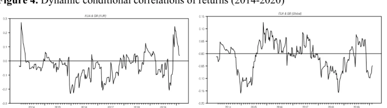
Figure 4. Dynamic conditional correlations of returns (2014-2020)
The correlation between EUA and GB returns are slightly less than zero according to the mean values in Table 4, and the standard deviation of their dynamic correlations are similar to zero, which implies that the volatility of EUA market has a lower effect on the volatility f green bond market. Specifically, the correlation degree between EUA and GB (EUR) appears the highest on average based on the mean values. Moreover, the correlation between EUA and GB is highly time-varying both within the timeframe of one year (e.g. 2014, 2016 and 2019) and across the full sample period. The correlation coefficient oscillates at a low level in the beginning of 2014, but the coefficient declines from February 2014 to reach a peak of -0.04 (EUA and GB (EUR)) and -0.17 (EUA and GB (Global)) in the end of 2014. The slowdown in economic activity which has exacerbated the surplus of emission allowances and the carbon market crisis is reflected in the decline of the correlation coefficient at the beginning of 2014, and it varies in the range of 0.01–0.12 from 2014 to 2018. Since the beginning of 2019, the dynamic conditional correlations between EUA and GB indices fluctuate around negative
correlations. This can be explained by the good performance of the carbon market in 2019 due to the fall in emissions in electricity production and the commissioning of the Market Stability Reserve mechanism (MSR), a sort of central allowance bank, intended to " to dry up " too
abundant supply of quotas and to support prices. When comparing Figures 1, 2 and 3, we
notice that the correlation between markets tends to increase as the market is more volatile. Besides, EUA and GB markets, confronted to uncertain information, have some risk complementarity effect. In particular, as shown in Figure 2, we can find that in addition to a few positive values, the dynamic conditional correlations between EUA and GB market returns are negative. This is an indication of consistency in the changes of time-varying variances between these two markets. Consequently, the risk separation may also change based on the rise or decline of the dynamic correlation coefficient.
4.3.2. Spillover effects
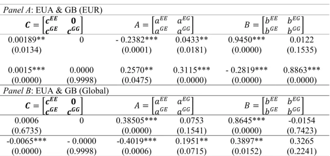
Table 5 provides the estimated results of the full BEKK-GARCH (1,1) model. The majority of conditional variances have been found to be statistically significant. This indicates that the current volatility of EUA market and GB depend on past shocks (𝑎 and 𝑎 ) and the past volatilities (𝑏 and 𝑏 , except for GB (global)). It implies that any unexpected events in the EUA market or green bond market can increase the implied volatility of their own markets. Investigating the off-diagonal elements of matrices A and B, 𝑎 and 𝑏 , i ≠ j, which capture cross-market effects, namely shock and volatility spillovers, respectively, between EUA and GB indexes, we find evidence of bi-directional shock transmission effects between EUA and GB (EUR), since the off-diagonal parameters, 𝑎 and 𝑎 , are both statistically significant. However, since 𝑏 is significantly negative, while 𝑏 is insignificant, past conditional volatility of GB (EUR) negatively affects the current level of EUA volatility.
Regarding the relationship between EUA and GB (Global), the significant 𝑎 coefficient estimate and insignificant 𝑎 parameter estimate suggest the existence of a uni-directional shock spillover from GB (Global) market to EUA market. Consequently, previous shocks of GB (Global) have a negative impact on the current volatility of EUA. Moreover, we find evidence of one-way positive volatility spillover effect from GB (Global) to EUA since 𝑏 is significantly positive and 𝑏 is insignificant.
Table 5. Estimation results of BEKK-GARCH model Panel A: EUA & GB (EUR)
𝑪 = 𝒄𝑬𝑬 𝟎 𝒄𝑮𝑬 𝒄𝑮𝑮 𝐴 = 𝑎 𝑎 𝑎 𝑎 𝐵 = 𝑏 𝑏 𝑏 𝑏 0.00189** (0.0134) 0 - 0.2382*** (0.0001) 0.0433** (0.0181) 0.9450*** (0.0000) (0.1535) 0.0122 0.0015*** (0.0000) (0.9998) 0.0000 0.2570** (0.0475) 0.3115*** (0.0000) - 0.2819*** (0.0000) 0.8863*** (0.0000)
Panel B: EUA & GB (Global)
𝑪 = 𝒄𝑬𝑬 𝟎 𝒄𝑮𝑬 𝒄𝑮𝑮 𝐴 = 𝑎 𝑎 𝑎 𝑎 𝐵 = 𝑏 𝑏 𝑏 𝑏 0.0006 (0.6735) 0 0.38505*** (0.0000) 0.0753 (0.1541) 0.8645*** (0.0000) -0.0154 (0.7423) -0.0065*** (0.0000) - 0.0000 (0.9998) -0.4019*** (0.0006) 0.1951** (0.0715) 0.3897** (0.0152) 0.3265 (0.2241)
Note: Log likelihood values are 2231.4752 and 2067.1764 for EUA & GB (EUR) and EUA & GB (Global) models, respectively. Values between parentheses are p-values.
V. Conclusion
This chapter examines the interaction between the carbon market and the green bond market in Europe by comparing their price and volatility dynamics over a six-year period corresponding to the Phase III of EU ETS (2014-2019).
To the best of our knowledge, it is the first attempt to compare the price volatility dynamics of the European Green Bond market and this of the European carbon market during this extensive period, where the EUA (auctioned) has an initial price.
Our methodological approach is based on two principles. First, we use the European prices of green bond and carbon indices rather than those of stock exchanges to track the evolution of prices and their returns. Second, we develop a VAR BEKK GARCH model that is revealed adequate to capture volatility shocks as well as volatility spillover effects from the European carbon market towards the European Green bond (GB) market and vice versa.
Our contribution to the literature is threefold. First, we report significant short-run and long-run persistence of shocks to the dynamic conditional correlation between European carbon and European green bond markets. By contrast, this persistence of shocks is insignificant on the short-term and on the long-term if we consider the case of European carbon and the Global green bond markets. Second, we find that the correlation coefficient between EUA and European Green bond markets is really low approaching zero. It tends to be slightly negative from the year 2019 because of the good carbon market performance due to the drop in emissions of electricity producers and the use of the Market Stability Reserve, intended to reduce too abundant supply of EUAs maintain EUA prices at a certain level. Third, we document bi-directional shock transmission effects between EUA and GB (EUR) in contrast to one-way positive volatility spillover effect from GB (Global) to EUA.
In sum, these results indicate that the green bonds issued in Europe may be used to hedge against the EUA carbon price (volatility) risk. This finding is important for investors and for fund managers that may purchase green bonds and EUA futures to create a portfolio of environmental assets. In this respect, these assets can be considered as complementary.
VI. Bibliography
Alberola, E. Chevallier, J. & Chèze, B. (2008). Price drivers and structural breaks in European carbon prices: 2005-2007. Energy Policy, Vol. 36, Issue 2, pp. 787-797.
Bachelet, M.J, Becchetti, L. & Manfredonia, S. (2018). The Green Bonds Premium Puzzle: The Role of Issuer Characteristics and Third-Party Verification. Sustainability, Vol. 11, Issue 4, pp.1-22.
Boutabba, M.A. (2009). Dynamic linkages among European carbon markets. Economic Bulletin, Vol. 29, Issue 2, pp. 499-511.
CBI (2019). Green Bond Pricing in the Primary Market January - June 2019, Harrison, C. CBI/HSBC (2016). Bonds and Climate Change: The State of the Market in 2016, July
Chevallier, J. & Ielpo. F. & Mercier. L. (2009). Risk aversion and institutional information disclosure on the European carbon market: a case study of the 2006 compliance event. Energy Policy, Vol. 37, Issue 1, pp. 15-28.
Engle, R.F., Kroner, K.F. (1995). Multivariate simultaneous generalized ARCH. Econometric Theory, Vol.11, pp.122-150.
Engle, R. (2002). Dynamic conditional correlation: a simple class of multivariate generalized autoregressive conditional heteroskedasticity models. Journal of Business and Economic Statistics, Vol. 20, Issue 3, pp. 339-350.
European Commission (2013). Commission Regulation No 389/2013 of 2 May 2013 establishing a Union Registry pursuant to Directive 2003/87/EC. Decisions No 280/2004/EC and No 406/2009/EC of the European Parliament and of the Council and repealing Commission Regulations (EU) No 920/2010 and No 1193/2011
Febi, W. Schäfer, D. Stephan, A. & Sun, C. (2018). The impact of liquidity risk on the yield
spread of green bonds. Finance Research Letters,Vol.27, pp.53-59.
Lucia. J. Mansanet-Bataller & M. Pardo. Á. (2015). Speculative and hedging activities in the European carbon market. Energy Policy, Vol. 82, July 2015, pp. 342-351
Medina V. & Pardo. A. (2013). Is the EUA a new asset class? Quantitative Finance. Vol.13 Issue 4. 637-653.
Mirova (2018). Liquidity of the Green Bond Market. Report published on February 20, 2018. Mizrach. B. (2012). Integration of the global carbon markets. Energy Economics, Vol.34, Issue
1. pp.335-349.
Monast. J. (2010). Climate change and financial markets: regulating the trade side of cap and trade. Environmental Law Reporter, Vol.40, Issue 1.
Neuhoff K. Schopp A. Boyd R. Stelmakh. K. & Vasa. A. (2012). Banking of surplus emissions EUAs: does the volume matter? Discussion Papers of DIW Berlin 1196.
Rannou, Y. & Barneto, P. (2016). Futures trading with information asymmetry and OTC predominance: Another look at the volume/ volatility relations in the European carbon markets. Energy Economics, Vol.53, pp.159–174.
Rannou, Y. (2019). Limit order books, uninformed traders and commodity derivatives: Insights from the European carbon futures. Economic Modelling, Vol.81, pp.387-410.
Rittler, D. (2012). Price discovery and volatility spillovers in the EU emissions trading scheme: a high frequency analysis. Journal of Banking and Finance, Vol.36, Issue 3, pp. 774-785. Stefan, M. & Wellenreuther, C. (2020). London vs. Leipzig: Price discovery of carbon futures
during Phase III of the ETS. Economics Letters, Vol. 188, 108990.
Tang, D.Y. & Zhang, Y. (2020). Do shareholders benefit from green bonds? Journal of Corporate Finance, Vol. 61, 101427.
Zerbib, O.D. (2019). The effect of pro-environmental preferences on bond prices: Evidence from green bonds. Journal of Banking and Finance, Vol. 98, pp.39-60.