A cautious approach to generalization in reinforcement learning
Texte intégral
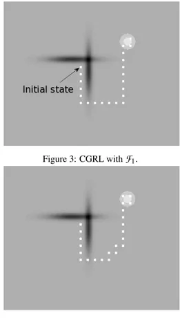
Figure


Documents relatifs
In this article, we propose a generalization of the classical finite difference method suitable with the approximation of solutions in subspaces of the Sobolev spaces H −s , s >
En 2015, 168 710 personnes se sont inscrites à Pôle emploi à la suite d’un licenciement économique ; parmi ces inscriptions, 107 400 se sont faites dans le cadre du CSP
Finale- ment, pour ce qui est du nombre de comprimés ou de suppositoires antinauséeux complémentaires pris dans chaque groupe, les patients du groupe halopéridol
We will show that the maximum of the volume product is attained at a metric space such that its canonical graph is a weighted complete graph.. In dimension two we can say
In non-archimedean geometry (in the sence of Berkovich), we a priori have a structure sheaf which is the analogy of the sheaf of holomorphic functions.. Apply- ing the
Berkovich’s strategy is based on the fact that in the case of a local non-Archimedean ground field with non-trivial absolute value, the Bruhat-Tits building of the group PGL(V)
Firstly, we develop a theory of designs in finite metric spaces that replaces the concept of designs in Q-polynomial association schemes, when the considered met- ric space does
We point out that eigenvalue problems involving quasilinear nonhomogeneous problems in Orlicz- Sobolev spaces were studied in [12] but in a different framework.. in [10, 11]
