Saliency Maps of High Dynamic Range Images

Roland Br´emond and Josselin Petit and Jean-Philippe Tarel

Universi´e Paris Est, LEPSiS, INRETS-LCPC {bremond,petit,tarel}@lcpc.fr

Abstract. A number of computational models of visual attention have been proposed based on the concept of saliency map. Some of them have been validated as predictors of the visual scan-path of observers looking at images and videos, using oculometric data. They are widely used for Computer Graphics applications, mainly for image rendering, in order to avoid spending too much computing time on non salient areas, and in video coding, in order to keep a better image quality in salient areas. However, these algorithms were not used so far with High Dynamic Range (HDR) inputs. In this paper, we show that in the case of HDR images, the predictions using algorithms based on Itti et al. (1998) are less accurate than with 8-bit images. To improve the saliency computation for HDR inputs, we propose a new algorithm derived from Itti & Koch (2000). From an eye tracking experiment with a HDR scene, we show that this algorithm leads to good results for the saliency map computation, with a better fit between the saliency map and the ocular fixation map than Itti et al.’s algorithm. These results may impact image retargeting issues, for the display of HDR images on both LDR and HDR display devices.

Key words: Saliency Map, High Dynamic Range, Eye Tracking

1

Introduction

The concept of visual saliency was introduced in the Image community by the influential paper of Itti, Koch & Niebur [1]. The purpose of these algorithms is to compute, from an image, a Saliency Map, which models the image-driven part of visual attention (gaze orientation), for observers looking at the image. In the same last ten years, High Dynamic Range imaging emerged as a new field of research in image science, including computer graphics, image acquisition and image display [2]. Eight-bit images are not the only way to deal with digital images, since techniques have been proposed to capture, process and display HDR images.

In this paper, we show that a direct computation of the saliency map using algorithms derived from [1] leads to poor results in the case of HDR images. We propose a new algorithm derived from Itti and Koch [3], with a new definition of the visual features (intensity, colour and orientation), which leads to better results in the case of HDR images. The saliency maps computed with our algo-rithm and with [3] are compared to human Region of Interest (RoI), using an eye tracker experiment.

Previous work on visual saliency computation are reviewed in section 2. Ev-idence for the drawback of Itti and Koch’s model for HDR images are given in section 3, as well as our alternative model. An eye tracker experiment is presented in section 4, allowing to compare the two computational models.The results are discussed in section 5.

2

Previous Work

Among several theories of visual attention, the Feature Integration Theory (FIT) [4] was made popular by [1] because it leads to an efficient computational model of the bottom-up visual saliency. Other biologically plausible implementations of the saliency map have been proposed, and some authors include computational models of top-down biases (see [5] for a review).

Itti et al.’s model [1], further refined in [3], tries to predict the bottom-up component of visual attention, which is the image-driven contribution to the gaze orientation selection. They implement the FIT using Koch & Ullman’s hypothesis of a unique saliency map in the spatial attention process [6]. This model was tested against oculometric data, and proved to be better than random at predicting ocular fixations [3].

Itti and Koch’s algorithm [3] is seen as the standard model for the compu-tation of the saliency map in still images. It extracts three early visual features from an image (intensities, opponent colours and orientations), at several spatial scales. This computation is followed by center-surround differences (implemented as Gaussian Dyadic Pyramid) and a normalization step for each feature. Next, an across-scales combination and a new normalization step lead to the so-called conspicuity map for each feature. The normalizations are computed as follows: a conspicuity map is iteratively convolved by a Difference of Gaussian (DoG) fil-ter, the original map is added to the result, and negative values are set to zero. Then, a constant (small) inhibitory term is added. Finally, the three conspicuity maps (Intensity, Colour and Orientation) are added into the saliency map (see [3] for implementation details). Other saliency algorithms, such as [7, 8] use the same principles derived from [1]: selection of the visual features, center-surround differences, competition across features, and fusion of the conspicuity maps into the saliency map.

Saliency maps have been widely used in the recent years for Computer Graph-ics applications, mostly in order to save computing time in rendering algorithms [9, 10]. Video coding applications have also emerged, keeping a better image quality in salient areas [11]. All these applications compute saliency maps using models derived from [1], with Low Dynamic Range (LDR) images. The present paper addresses the computation of saliency maps for HDR images, which has implications for both LDR and HDR display devices.

3

Saliency Maps of HDR Images

We have extended the Saliency Toolbox for Matlab [12] available online [13] to HDR input (float images). Alternative algorithms, such as [14] were not tested, so that our findings are restricted to Itti’s computational strategy, which is the most popular in computer science, and led to the more convincing oculometric validations.

3.1 Drawback of the Standard Model

Focusing on biologically inspired algorithms derived from [1], it appears that a direct computation of the saliency map may lead to poor results for HDR images in terms of information: the saliency map selects the most salient item, loosing information about other salient items.

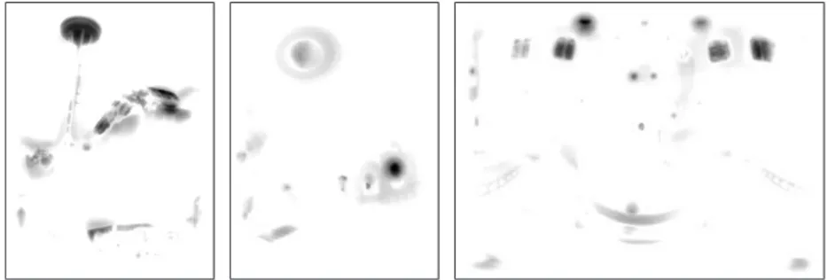
Fig. 1. Space Needle (left), Memorial Church (middle) and Grace New (right) HDR images. Top: LDR tone mapped images. Bottom: Saliency maps computed from the HDR images.

Fig. 1 (top) gives two examples of saliency maps computed with [3] from 32-bit HDR images from Debevec’s website [15]. As HDR images cannot be printed, they are displayed (Fig. 1, bottom) after being tone mapped into LDR images [16]. These examples suggest that a direct computation of the saliency map looses relevant information, as far as visual attention is concerned. In the Grace New image, only windows and light sources are selected. The saliency map aims at predicting the visual behavior: one may doubt that observers would

only look at light sources and windows in the HDR scene. This is even worst with the Memorial Church HDR image, where the saliency map only selects one window in the church. From these limited examples (more examples are available as supplementary material of the present paper), it seems that state-of-the art saliency map algorithms tend to select the most salient items in a HDR scene, the other salient items being either faded, or removed. These ”poor” saliency maps of HDR images do not correspond to the actual visual behavior.

3.2 Contrast vs. Difference

A naive approach would be to compute the saliency maps after a tone mapping preprocessing (see section 3.3), however we were looking for a unified approach, which proved to give better result than the two-steps approach (see section 4.2). Looking carefully at the conspicuity maps of HDR images, we found that the color map seems to include more information than the two others. This observation suggested an hypothesis. When the feature maps are computed in [3], the Colour feature is normalized, at every pixel, with respect to intensity I, whereas the Intensity and Orientation features process differences (between spatial scales). Knowing that biological sensors are sensitive to contrasts rather than to absolute differences, we felt that the saliency map of HDR images would benefit from a computational model in terms of contrast on all three conspicuity maps (Intensity, Colour and Orientation). This normalization may be seen as a gain modulation, which is the physiological mechanism of visual adaptation.

Thus, we replace the Intensity channel in [3]. Instead of computing the in-tensity difference between scales c and s: I(c, s) = |I(c) − I(s)|, we compute an intensity contrast:

I′_{(c, s) =} |I(c) − I(s)|

I(s) (1)

(a) (b) (c)

Fig. 2.Contour detection in (a) with (b) normalized Gabor filters (our proposal), and (c) differences of Gabor filters at successive scales, as in [3].

Then, we propose a modification of Itti et al.’s definition of the Orientation features, so that the new feature is homogeneous to a contrast. In the original paper, orientation detectors were computed, for each orientation angle θ, as differences between Gabor filters at scales c and s: O(c, s, θ) = |O(c, θ)−O(s, θ)|. This leads to orientation detectors where the borders themselves are not detected

(see Fig. 2). Instead, we see a propagation across scales of what is actually detected: borders of borders. This observation, added to the fact that a Gabor filter is a derivative filter, led us to a new definition of the Orientation features:

O′_{(c, s, θ) =}O(c, θ)

I(s) (2)

with a normalization over the intensity channel, as for the two other features. Fig. 3 shows examples of saliency maps computed for HDR images with this new operator, denoted CF (for Contrast Features) in the following, without the strong drawback of Fig. 1.

Fig. 3. Saliency maps of the Space Needle, Memorial Church and Grace New HDR images computed with the CF algorithm, with new definitions of the Intensity and Orientation features.

In order to check the consistency of the CF algorithm for LDR images, we also compared the saliency map of the LDR images, computed with [3] and with the proposed algorithm. An example is given Fig. 4 for the Lena picture, showing that the saliency maps are close to each other for LDR inputs.

(a) (b) (c)

Fig. 4.Saliency maps of Lena (a), computed with (b) [3] and with (c) the CF algo-rithm.

3.3 Tone Mapping preprocessing

Usual sensors, either physical or biological, cope with the high dynamic range of input luminance by means of a non-linear sensitivity function, allowing to

shrink the luminance dynamic into a LDR output dynamic: all sensors include a Tone Mapping Operator (TMO). Thus, one may argue that the apparent failure of [3] for HDR images comes from the HDR input data. One may expect that reproducing sensors properties and mapping HDR images to LDR images before computing a saliency map would lead to better results than without this preprocessing step.

A number of TMO have been proposed so far in the Computer Graphics literature. Please note that in the following, we use TMO for a task which is not the usual rendering task. Instead of comparing the visual appearance of tone mapped images, we use them in order to compute accurate saliency maps. In section 4.2, we have compared our algorithm to six such operators from the literature, combined with a saliency map computed with [3]:

– Tumblin and Rushmeier [17] (denoted O1), based on psychophysical data,

tries to keep the apparent brightness in the images.

– Ward et al. [18] (denoted O2) uses a histogram adjustment method (we did

not consider the colour processing, nor the glare simulation of the operator), trying to keep the contrast visibility in the images.

– Pattanaik et al. [19] (denoted O3) uses a colour appearance model (we used

the static version of the operator).

– Reinhard et al. [16] (denoted O4) uses a method inspired by photographic

art (we use the global version of the operator).

– Reinhard and Delvin [20] (denoted O5) is inspired by photobiology.

– Mantiuk et al. [21] (denoted O6) optimizes tone mapping parameters in terms

of visibility distortion, using Daly’s Visual Difference Predictor (VDP) [22]. Given that these operators may be sensitive to the parameter tuning, we have used the default parameters as described in the cited publications.

4

Experiment

In order to test the relevance of a given saliency map computation for HDR images, a ground truth is needed. This was done on a limited scale in a psycho-visual experiment, with a HDR physical scene, collecting oculometric data.

In the general case, one may consider the saliency map as an input for the top-down biases in the attention process. However, we followed [3, 23, 11] and did not considered such top-down biases. Instead, we used the saliency map as a predictor of the gaze orientation, in an experiment where the visual task was chosen in order to avoid strong top-down biases. Thus, the fixation map could be compared to predictions from these saliency maps.

We have designed an eye tracking experiment to test our hypothesis about the visual behavior looking at HDR scenes. The ocular fixations of 17 observers looking at a physical HDR scene were recorded. Then, the scene was scanned with a camera with various exposures, in order to build a HDR image. This allowed to compute various saliency maps from the HDR image.

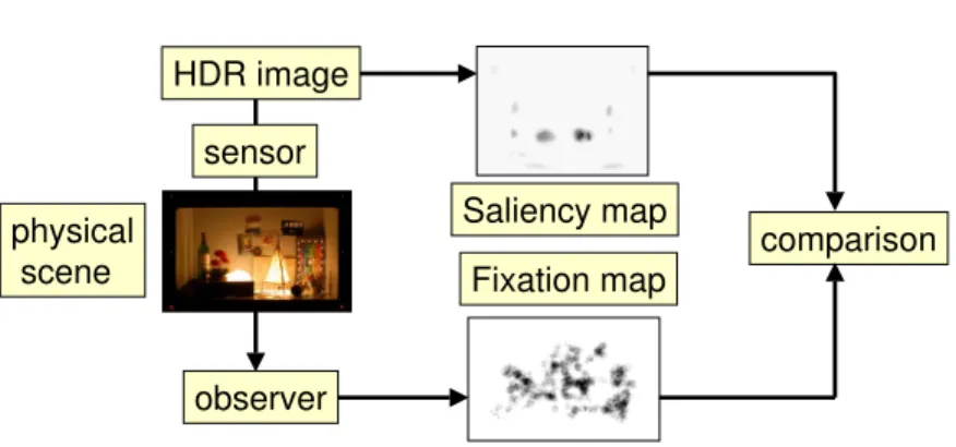
observer Saliency map Fixation map comparison sensor HDR image physical scene

Fig. 5.Framework of the Saliency Map evaluation for HDR images.

4.1 Material and Method

The experiment took place in a dark room (no windows, walls painted in black) under controlled photometry. The scene (Fig. 7, right) included dark (small box, yoghurt) and bright parts (lamps), leading to a luminance dynamic of 3,480,000:1 and very strong contrasts (the yoghurt and the open box are near the light sources). The scene was installed in a closed box (except for the front part, see Fig. 6).

observer

eye tracker

scene box video-projector

Fig. 6.Experimental setup.

Subjects were seated in an ergonomic automobile seat, allowing to adjust the eye height and to minimize head movements. The scene box angular size was 20◦_{. Ocular fixations were recorded using a SMI X-RED distant eye tracker.}

Eight LEDs around the box served for the eye-tracker calibration, together with a central LED in the middle of the box, with a physical protection around, avoiding that any light would make the scene visible during the calibration. A video-projector displayed light on the back wall, avoiding possible glare due to the lamps in the scene box, however without light reflexion inside the box.

Seventeen subjects participated to the experiment (11 men, 6 women, mean age 29). Although some of them worked in the field of digital image, they were naive to the purpose of the experiment. They were asked to look freely at the scene during 30 s. We followed [23], telling them that they would be asked a very

general question at the end of the experiment. Altogether, these instructions avoided strong task-dependent biases.

A black curtain hid the scene during the first part of the experiment (subjects entering the room, seating, seat adjustment in height, explanations about the experiment). Then, the light was turned off in the room, the curtain was opened, and the eye tracker was calibrated using the LEDs as reference fixation points. Finally, the LEDs were powered off, the scene box was lit, and the eye tracker record began. In the end, subjects were asked to mention the main objects they had noticed in the scene (these data are not analyzed here).

4.2 Results

We followed Le Meur et al. [11] and computed a Regions of Interest (RoI) map from the subject’s fixations in the first 30 s. Fixations were defined as discs of 1◦ _{radius, where the gaze stayed for at least 100 ms. All fixation patterns (for}

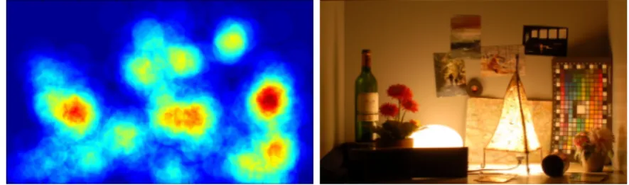
the 17 subjects) were added together, providing a spatial distribution of human fixations. The RoI map is a probability distribution of the gaze direction, so its integral is normalized to 1. Fig. 7 (left) shows the RoI map obtained from individual fixations. Compared to the saliency maps of Fig. 8, the RoI map is smoother, which sets some limits to further comparisons.

Fig. 7.Left: Fixation map (RoI) recorded over the individual fixations of 17 observers, in false colours. Right: : LDR (JPEG) photograph of the HDR scene.

The next step was to compute saliency maps out of the experimental scene. First, photographs were taken with various integration times (bracketing) from the observer’s position, in order to build a HDR image [24] close to what ob-servers actually looked at. Saliency maps were computed out of this image, using both [3] and the CF algorithm. We also computed, for comparison, saliency maps using [3] after preprocessing with O1 to O6 (see section 3.3). Fig. 8 shows the

resulting saliency maps in false colours.

Comparing the saliency maps suggests that some items which were missed by [3] were found by the CF algorithm, such as the yoghurt, the black box, the top right photograph, while the wine bottle is enphasized (see Tab. 1 for quantitative evidence). As expected, the direct saliency map computation with

CF [Itti 2000]

O1 + [Itti 2000] O2 + [Itti 2000] O3 + [Itti 2000]

O4 + [Itti 2000] O5 + [Itti 2000] O6 + [Itti 2000]

Fig. 8. Saliency maps of the experimental HDR scene computed with the proposed CFalgorithm, and with [3] without and with preprocessing O1−O6.

[3] only selects the two lamps and the colour chart (the colour feature is the only one to be normalized, see section 3.2).

An unexpected result is that some TMO fail in capturing more areas of interest than the direct saliency map computation with [3] (see O5for instance).

Another interesting point is the strong difference between the saliency maps, depending on the TMO preprocessing. For instance, most TMO allow to capture the yoghurt (bottom right of the image) which is not detected by the direct computation, however O2and O6emphasize the left lamp, while O2, O4and O6

emphasize the wine bottle, O5 captures the top right photograph, etc.

The RoI only contains low spatial frequencies, partly due to accuracy issues in the eye tracking methodology. Thus, a direct quantitative comparison be-tween the RoI and saliency maps is meaningless, as far as high frequencies are concerned. We took this limitation into account using the same 1◦_{dilatation for}

the saliency maps as was previously done for the RoI, before any quantitative comparison. Then, we assumed that both the saliency maps and RoI map are probability distributions, and thus normalized in consequence.

Two criteria were used for the comparison. The first one is the square root eof the Mean Square Error (MSE) between the saliency and RoI distributions (see Tab. 1). However, as the MSE is a global criterion averaging on many pixels, we also used a finer comparison criterion based on level sets. For any probability value t between 0 and 1, saliency and RoI binary images can be built by thresholding the saliency and RoI distributions, and then compared. To

compare two binary images, we used the Dice coefficient, which is relevant when the relative surface of the target is small:

s= 2 × T P

2 × T P + F P + F N (3)

where T P = True Positive, F P = False Positive and F N = False Negative pixels. The higher the Dice coefficient, the more similar the binary images. This leads to curves of the Dice coefficient s versus the threshold probability value t, as shown in Fig. 9. If the Dice curve obtained for one algorithm is always higher than the one obtained for another algorithm, the first one performs better.

Algo. 104 erank s rank [3] 6.15 [6] 0.127 [6] CF 4.63 [1] 0.161 [1] O1 + [3] 4.65 [2] 0.158 [3] O2 + [3] 5.47 [5] 0.131 [5] O3 + [3] 7.67 [8] 0.093 [8] O4 + [3] 4.89 [3] 0.160 [2] O5 + [3] 6.22 [7] 0.126 [7] O6 + [3] 5.36 [4] 0.145 [4]

Table 1.Error indexes e and s comparing the RoI and the saliency maps, depending on the algorithm (rank in brackets).

Fig. 9.Dice coefficient for the CF Saliency Map and [3] when compared to the RoI map, with threshold t as parameter.

When comparing MSE values and mean Dice coefficients (see Tab. 1), the CFalgorithms ranks first in both cases (the rank does not change much whether we use the MSE or the Dice). The square root of the MSE is improved by 33% compared to [3], while the mean Dice is improved by 27%. Besides, none of the

TMO, used as preprocessing before [3], managed to perform better than the proposed CF algorithm in the tested situation. Furthermore, the tested TMO not always lead to a more predictive saliency maps than a direct saliency map computation without TMO, which is a counter-intuitive result. For instance, using O3and O5before [3] is worst than [3] alone.

5

Conclusion

We have focused on a drawback of the most popular computational models of the visual saliency when applied to HDR images. This can be put in terms of missing information: a direct saliency maps computation is poorly predictive of the gaze orientation. We have proposed a new algorithm, improving the saliency map quality on HDR images, that is, leading to a better fit with oculometric data. This CF algorithm was rated best in terms of the Dice coefficient and in terms of MSE, compared to [3]. In addition, it gives better results than 6 TMO from the literature (in order to compress the image dynamic) followed by [3]. This last result suggests that the drawback of Itti and Koch’s standard model for HDR images is not due to the input image interpretation, but more probably to the feature’s definition. Note that the standard feature definitions perform well on LDR images, and the need for modified features is limited to HDR images.

These results may benefit to HDR video coding and HDR display, as a num-ber of compression and processing algorithms already use bottom-up saliency computations in order to optimize the computing time and compression rate. Thus, a more reliable computation of the bottom-up saliency of HDR input images should improve the quality of the displayed image.

Still, a predictive model of human fixations is beyond the possibility of such bottom-up saliency models [25]. This is emphasized by the fact that the Dice coefficients (Tab. 1 and Fig. 9) are quite low, whatever the method. This is partly due to the fact that visual attention is not only driven by the bottom-up visual saliency. In search for a more predictive model, alternative approaches may also compute the top-down component of visual attention, providing that a semantic description of the scene is available, which is often the case in Computer Graphic applications. For instance, Navalpakkam and Itti used the scene gist and a priori knowledge about the current task in order to bias the bottom-up saliency [26], while Gao and Vasconcelos computed a discriminant saliency linked to object recognition [27].

References

1. Itti, L., Koch, C., Niebur, E.: A model of saliency-based visual attention for rapid scene analysis. IEEE Transactions on Pattern Analysis and Machine Intelligence 20(1998) 1254–1259

2. Reinhard, E., Ward, G., Pattanaik, S.N., Debevec, P.: High dynamic range imaging: acquisition, display, and image-based lighting. Morgan Kaufmann (2005)

3. Itti, L., Koch, C.: A saliency-based search mechanism for overt and covert shifts of visual attention. Vision Research 40 (2000) 1489–1506

4. Treisman, A.M., Gelade, G.: A feature-integration theory of attention. Cognitive Psychology 12 (1980) 97–136

5. Itti, L., Rees, G., Tsotsos, J.K.: (Ed.) Neurobiology of attention. Elsevier (2005) 6. Koch, C., Ullman, S.: Shifts in selective visual attention: towards the underlying

neural circuitry. Human Neurobiology 4 (1985) 219–227

7. Choi, S.B., Jung, B.S., Ban, S.W., Niitsuma, H., Lee, M.: Biologically motivated vergence control system using human-like selective attention model. Neurocom-puting 69 (2006) 537–558

8. Parkhurst, D., Law, K., Niebur, E.: Modeling the role of saliency in the allocation of overt visual attention. Vision Research 42 (2007) 107–123

9. Reddy, M.: Perceptually optimized 3D graphics. IEEE Computer Graphics and Applications 22 (2001) 68–75

10. Lee, C.H., Varshney, A., Jacobs, D.W.: Mesh saliency. ACM Transactions on Graphics 24 (2005) 659–666

11. LeMeur, O., LeCallet, P., Barba, D., Thoreau, D.: A coherent computational approach to model bottom-up visual attention. IEEE Transactions on Pattern Analysis and Machine Intelligence 28 (2006) 802–817

12. Walther, D., Koch, C.: Modeling attention to salient proto-objects. Neural Net-works 19 (2006) 1395–1407

13. Walther, D.: http://www.saliencytoolbox.net/ (2006)

14. Bruce, N., Tsotsos, J.K.: Saliency based on information maximization. Advances in Neural Information Processing Systems 18 (2006) 155–162

15. Debevec, P.: http://gl.ict.usc.edu/data/ (00)

16. Reinhard, E., Stark, M., Shirley, P., Ferwerda, J.: Photographic tone reproduction for digital images. In: Proceedings of SIGGRAPH. (2002)

17. Tumblin, J., Rushmeier, H.: Tone reproduction for realistic images. IEEE computer Graphics and Applications 13 (1993) 42–48

18. Ward, G., Rushmeier, H., Piatko, C.: A visibility matching tone reproduction operator for high dynamic range scenes. IEEE Transactions on Visualization and Computer Graphics 3 (1997) 291–306

19. Pattanaik, S.N., Tumblin, J., Yee, H., Greenberg, D.P.: Time-dependent visual adaptation for fast realistic image display. In: Proceedings of SIGGRAPH, ACM Press (2000) 47–54

20. Reinhard, E., Devlin, K.: Dynamic range reduction inspired by photoreceptor physiology. IEEE Transactions on Visualization and Computer Graphics 11 (2005) 21. Mantiuk, R., Daly, S., Kerofsky, L.: Display adaptive tone mapping. ACM

Trans-actions on Graphics 27 (2008) article no. 68

22. Daly, S. In: The visible differences predictor: an algorithm for the assessment of image fidelity. A. B. Watson Ed., Digital Images and Human Vision, MIT Press, Cambridge, MA (1993) 179–206

23. Itti, L.: Automatic foveation for video compression using a neurobiological model of visual attention. IEEE Transactions on Image Processing 13 (2004) 1304–1318 24. Debevec, P., Malik, J.: Recovering high dynamic range radiance maps from

pho-tographs. In: Proceedings of ACM SIGGRAPH. (1997) 369–378

25. Knudsen, E.I.: Fundamental components of attention. Annual Review Neuro-science 30 (2007) 57–78

26. Navalpakkam, V., Itti, L.: Modeling the influence of task on attention. Vision Research 45 (2005) 205–231

27. Gao, D., Han, S., Vasconcelos, N.: Discriminant saliency, the detection of suspicious coincidences, and applications to visual recognition. IEEE Transactions on Pattern Analysis and Machine Intelligence 31 (2009) 989–1005