Applications of frequency combs in remote sensing
Thèse
Sylvain Boudreau
Doctorat en génie électrique
Philosophiæ doctor (Ph.D.)
Résumé
Cette thèse a pour objectif l’exploration des applications potentielles des peignes de fréquences en télédétection. Pour ce faire, trois configurations expérimentales sont étudiées. Pour chacune des configurations, une analyse de divers aspects de leur fonctionnement est faite et les avantages et les inconvénients qui y sont propres sont discutés. Des montages expérimentaux basés sur ces configurations ont été fabriqués en laboratoire. Des mesures expérimentales viennent démontrer les capacités de détection des différentes techniques.
La première configuration étudiée concerne l’échantillonnage passif d’une source optique externe. Cette technique permet d’évaluer le spectre de la source d’intérêt en la combinant interférométriquement avec les impulsions d’une paire de peignes de fréquences. Une étude probabiliste de la technique est effectuée afin d’en évaluer les limites de performance. Des mesures de sources cohérentes et incohérentes à haute résolution spectrale sont présentées.
La deuxième technique étudiée exploite la configuration dite incohérente permettant de faire la caractérisation active d’une cible. Cette technique rend possible la mesure hyperspectrale résolue en distance d’une scène observée. Un montage expérimental de lidar hyperspectral a été conçu et fabriqué en laboratoire dans le but de faire des mesures extérieures de cibles à une distance allant jusqu’à 175 m. Les capacités de détection de plusieurs caractéristiques de cibles sont démontrées pour des cibles dures et distribuées, sous forme de nuages d’aérosols. Des mesures de raies d’absorption moléculaire, ainsi que d’épaisseur d’échantillons transparents et translucides, sont présentées. La troisième configuration étudiée, dite cohérente, permet de faire de la mesure active d’une cible en utilisant un des trains d’impulsions comme oscillateur local. L’utilisation d’un oscillateur local ouvre la porte à des mesures de vibrométrie à haute sensibilité, ce qui est impossible en configuration incohérente. Un modèle analytique de collecte de puissance pour les systèmes à un seul mode transversal, permettant de prédire les puissances en jeu en configuration cohérente, est développé et validé expérimentalement. La technique de référencement habituelle, permettant de corriger les erreurs causées par les fluctuations des paramètres des peignes, est modifiée et adaptée aux mesures de vibrométrie cohérente. Des mesures de vibrométrie résolue en distance sont présentées, où la capacité du système à démoduler une voix humaine à partir des vibrations d’un mur est démontrée.
The goal of this thesis is to explore the potential applications of frequency combs for remote sensing. For this purpose, three comb-based configurations are studied. For each of these configurations, an analysis of their workings is performed and their advantages and disadvantages are discussed. Experimental setups based on those configurations were built in laboratory. The detection capabilities of the techniques are demonstrated through experimental measurements.
The first configuration that is studied enables passive sampling of an external optical source. Using this technique, it is possible to compute the spectrum of the considered source by interferometrically combining it with the pulses from a pair of frequency combs. A stochastic study of the technique is performed to assess its performance limits. Coherent and incoherent sources with high-resolution spectral content are measured.
The second technique uses a configuration called incoherent that enables active characterization of a target. Using this technique, it is possible to perform range-resolved hyperspectral measurements of an observed scene. A hyperspectral lidar setup was designed and assembled in laboratory with the goal of performing outdoors measurements of targets at distances up to 175 m. The sensing capabilities of the system are shown for hard and distributed targets, in the form of aerosol clouds. Molecular absorption measurements, as well as thickness measurements for both transparent and translucent targets, are shown.
Using the coherent configuration, which is the third one that was considered, it is possible to make active measurements of a target by using one of the pulse trains as a local oscillator. The use of a local oscillator opens the door to high sensitivity vibrometry, which is impossible with the incoherent configuration. An analytical model for the power collection capabilities of a single-transverse-mode system, which has to be used for coherent measurements, is developed and experimentally validated. The usual referencing technique, which is used to correct for fluctuations in comb parameters, is modified and adapted to the case of coherent vibrometry. Range-resolved vibrometry measurements are performed, demonstrating the capability of the system to extract a human voice signal from the vibrations of a wall.
Contents
Résumé ... iii
Abstract ... v
Contents ... vii
List of tables ... ix
List of figures ... xi
List of acronyms ... xvii
Remerciements ... xix
Introduction ... 1
1 Dual-comb interferometry ... 5
1.1 Single comb description ... 5
1.2 Two comb interferometry ... 9
1.2.1 Time domain representation ... 9
1.2.2 Frequency domain representation ... 12
1.2.3 Incoherent interferometry ... 18
1.2.4 Coherent interferometry ... 22
1.2.5 Sampling the peak of the photodetected pulses ... 25
1.3 Referencing algorithm... 26
1.3.1 Choosing grating length ... 30
1.3.2 Referencing with pulse picking... 33
1.4 Optical sampling by cavity tuning ... 36
1.4.1 Effect of dispersion in the delay line ... 38
1.4.2 Use of an acousto-optic modulator ... 41
2 Passive dual-comb spectroscopy ... 43
2.1 Description of a random optical source ... 44
2.2 Description of the sampling technique ... 45
2.3 Noise analysis ... 51
2.4 Estimation noise for a Fourier transform spectrometer ... 57
2.5 Experimental setup ... 60
2.6 Results ... 62
viii
3.1.1 Measurement configuration... 73
3.1.2 Range-resolved incoherent interferometry ... 74
3.1.3 Power collection ... 78
3.1.4 Performance metrics for hard and distributed targets ... 79
3.1.5 Pulse picking ... 81
3.2 Experimental setup ... 85
3.2.1 Fibre based section ... 85
3.2.2 Launching and light collection ... 94
3.3 Results ... 99
3.3.1 Short distance indoors measurements ... 99
3.3.2 Long distance outdoors measurements ... 113
4 Coherent vibrometry ... 141
4.1 Power collection ... 142
4.1.1 Model for power collection in a single mode system ... 142
4.1.2 Model validation ... 153
4.2 Voice detection with coherent vibrometry ... 161
4.2.1 Description of the technique ... 161
4.2.2 Modified referencing algorithm ... 165
4.2.3 Results ... 172
Conclusion ... 179
Bibliography ... 183
Appendix A. Interferometric photodetection of a complex Gaussian process ... 189
List of tables
Table 2-1. Signal-to-noise ratio for FTS and optical sampling spectroscopy ... 54
Table 2-2. Relevant values for optical sources power threshold calculation. ... 65
Table 2-3. Measured power for sampled and sampling sources. ... 66
Table 2-4 - Reference and measured frequencies of HCN absorption lines ... 70
Table 3-1. Component list for the referencing subsystem. ... 93
Table 3-2. Components list for the free space beam combiner. ... 95
Table 3-3. Specifications of the PLA-641 and PLA-841 APDs... 99
Table 3-4. Amplifier currents for samples at 10 m ... 100
Table 3-5. Measured thicknesses of the borosilicate glass stack components with a caliper and with the lidar system. ... 121
Table 3-6. Unambiguous ranging using the interferogram delay. ... 128
Table 3-7. Ranged distance compared to distance measured using the dual-comb interferogram. ... 128
Table 3-8. Position of peaks in the calibration interferogram for a stack of three glass slabs at 175 m. ... 133
Table 3-9. Measured vs rated thicknesses for the three-slab stack, assuming an index of 1.5 for each slab. ... 133
Table 4-1. Launched beam parameters extracted from the fit on collected power as a function of distance from the launcher for various beams. ... 157
List of figures
Fig. 1-1. Time domain representation of a frequency comb. ... 7 Fig. 1-2 Frequency domain representation of a frequency comb. ... 8 Fig. 1-3. Dual comb interferometry experiment in its simplest form. PD stands for
photodetector. ... 9 Fig. 1-4. Resulting beating signal at the output of a photodetector. Each electrical pulse is the
result of the interference between a pair of optical pulses, where its amplitude is the cross-correlation of the fields of both pulses at the relevent delay. ... 12 Fig. 1-5. Electrical beating between two combs in the frequency domain. Multiple copies of
both flipped and non-flipped version of the cross spectrum, are stacked in the electrical spectrum and amplitude modulated by the frequency response of the detector. In this case there is some overlap between flipped and non-flipped copies. ... 14 Fig. 1-6. Electrical beating with a frequency offset of 40 MHz. The positive and negative copies
are now well separated. ... 15 Fig. 1-7. First two copies of the cross-spectrum. The lowest frequency copy is not flipped,
while the highest frequency copy is. ... 18 Fig. 1-8. Schematic of the incoherent measurement experiment. ... 19 Fig. 1-9. Insensitivity to delay fluctuations in the incoherent configuration. Since both pulses
experience the vibration-induced delay, denoted Dv, their interferometric relation is not
modified. The position of the resulting electrical pulse is slightly changed, but this is most often negligible. ... 21 Fig. 1-10. Schematic of the coherent measurement experiment. ... 22 Fig. 1-11. Impulse response sampling interpretation of the coherent configuration. Every pulse
from the first comb is filtered by the sample, generating its impulse response. Every repetition period, the second comb samples that impulse response at uniformly spaced points... 23 Fig. 1-12. Schematic of the referencing setup. The combs are combined and filtered by two
fibre Bragg gratings, labeled FBG1 and FBG2, and photodetected. ... 28 Fig. 1-13. Original and correction sampling grids. The original sampling grid is uniform in k,
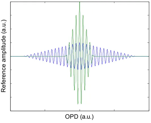
but non-uniform in effective sampling delay. By interpolating the k axis on a uniform grid from the second reference signal, the correction sampling grid is obtained. The signal interferogram can then be interpolated on that grid to remove OPD jitter. ... 30 Fig. 1-14. Ideal reference interferograms for two grating lengths, illustrating the compromise
between peak amplitude and OPD span. ... 32 Fig. 1-15. Measured interferograms of both reference gratings. The imperfections of the second
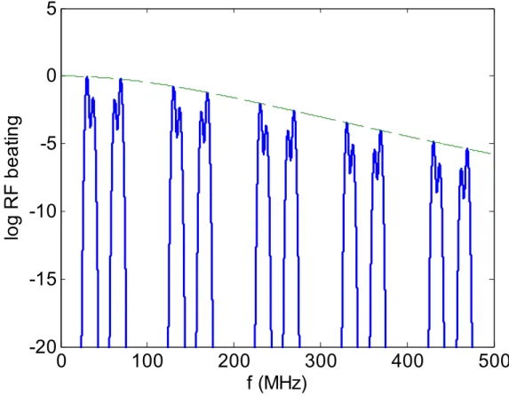
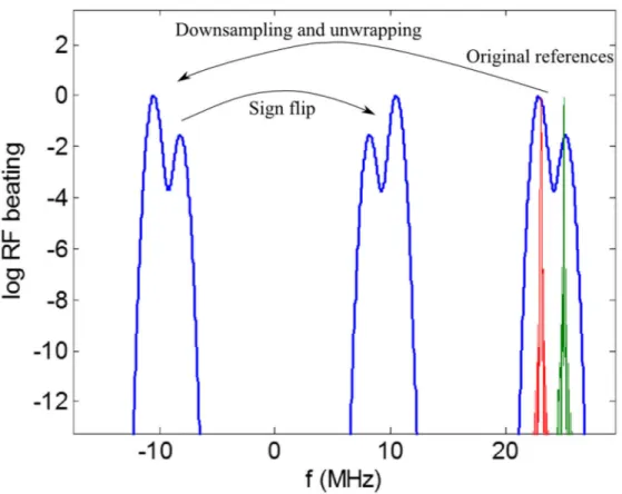
grating limit the effective referencing range to about ±7 cm. ... 33 Fig. 1-16. Synthetic spectra with a repetition rate of 100 MHz and a pulse picking factor of 3
xii
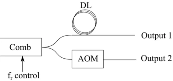
Fig. 1-18. Schematic of the OSCAT setup. One comb is split into two arms. One of those arm is fed to a delay line (DL). Both outputs can be used in the same configurations as the
outputs from the two combs in a dual-comb experiment. ... 36
Fig. 1-19. Illustration of the workings of the OSCAT configuration. The delay D causes each pulse to interact with a different pulse in the pulse train. Changing the pulse period, T, results in a different effective delay between interacting pulses. ... 37
Fig. 1-20. Pulse width as a function of propagation distance with a Gaussian input pulse and a linear group delay propagation medium. The green dotted line represents the linear asymptote. For short propagation distances, pulse width increases slowly, before reaching a point where pulse width becomes almost linear with propagation distance. ... 40
Fig. 1-21. Schematic of the OSCAT configuration with an acousto-optic modulator. ... 42
Fig. 2-1. In a Michelson interferometer, a source is split into two parts and recombined with variable lag using a movable mirror. A photodetector records the interferogram. ... 46
Fig. 2-2. Schematic of the measurement setup. The source is sampled by both combs and detected on balanced photodetectors (BPD). A wideband beating is also measured for alignment purposes. ... 46
Fig. 2-3. Ideal Dirac sampling picture of comb-based passive spectroscopy. Each pulse pair from the combs samples the source at lag τ[k]. ... 48
Fig. 2-4. Normalized SNR, by estimation noise SNR, for the three types of noise for a Fourier transform spectrometer measuring a 30 nm wide source centered at 1550 nm. ... 60
Fig. 2-5. Test setup for thermal stability. One comb is set to interfere with itself. Interference fringes in the self-beating indicate unsatisfactory thermal stability. ... 61
Fig. 2-6. Autocorrelation of the laser source ... 63
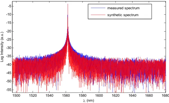
Fig. 2-7. Measured spectrum and synthetic spectrum with the expected amount of noise. ... 64
Fig. 2-8. Zoom on the laser line. ... 64
Fig. 2-9. Autocorrelation of the HCN filtered source. The clipped peak has a unitary amplitude. ... 67
Fig. 2-10. Squared signal-to-noise ratio of the autocorrelation estimate as a function of the number of averaged traces. ... 67
Fig. 2-11. Spectrum of the HCN filtered source. ... 69
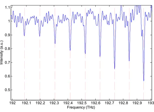
Fig. 2-12. Transmittance of the HCN cell. The red dotted lines mark the expected line positions. ... 69
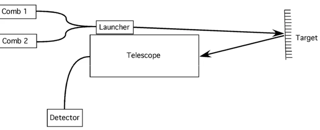
Fig. 3-1. Hyperspectral lidar in the incoherent configuration. Both combs are sent to the target. ... 72
Fig. 3-2. Synthetic target impulse response to a pulse pair for a delay τ. The red box represents the integration time of the photodetector. Here, the autocorrelation of the complete target response is measured. ... 75
Fig. 3-3. Synthetic target impulse response to a pulse pair for a delay τ. The photodetector integration time is small enough to resolve the two individual target components. ... 76 Fig. 3-4. a) Synthetic photodetected signal corresponding to a two event target. At every
repetition period, a new interferometrically modulated pulse pair is generated for a different OPD. b) Sliced version of the measured signal, with one dimension
corresponding to range and the other corresponding to OPD, highlighting the range
resolved interferometric information contained in the photodetected signal. ... 77
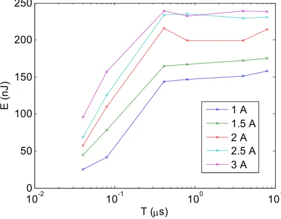
Fig. 3-5. Pulse energy at the output of one of the EDFAs as a function of pulse repetition interval. For all pumping currents, the pulse energy caps between 0.1 µs and 0.5 µs, resulting in an optimal repetition rate between 2 MHz and 10 MHz with respect to additive noise. ... 83
Fig. 3-6. Schematic of the experimental setup for hyperspectral lidar. ... 86
Fig. 3-7. Schematic of a pulse picker. ... 88
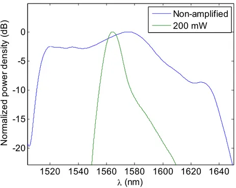
Fig. 3-8. Normalized power densities of a non-amplified comb and of a 200 mW amplified comb. ... 89
Fig. 3-9. Spectrum with output powers of 80 mW and 10 mW respectively for each comb. ... 91
Fig. 3-10. Spectrum with output powers of 540 mW and 690 mW respectively. Spectral fringes arising from non-linear effects break the calibration ... 91
Fig. 3-11. Complete fibre-based portion of the hyperspectral lidar setup. ... 94
Fig. 3-12. Schematic of the free space beam combiner. The two beams are combined on a beam splitter (BS) after their polarization has been linearized by a polarization beam splitter (PBS)... 95
Fig. 3-13. Signal attenuation due to geometric effects for a Lambertian target. ... 96
Fig. 3-14. Launching and collection system. The path of the launched beam is shown as a red line. ... 97
Fig. 3-15. Schematic of the camera co-registration setup. ... 98
Fig. 3-16. Pictures of a scene (left) and of the image captured by the infrared camera (right) side by side. The superposition of the image of the scene and the photodetector can be observed. ... 98
Fig. 3-17. Spectrum of a high-density polyethylene sample at 10 m. ... 102
Fig. 3-18. Calibrated IGM for the high-density polyethylene sample at 10 m. ... 102
Fig. 3-19. Interferential filter (5 degree angle) at 10 m. ... 104
Fig. 3-20. Channel spectrum delay for different angles of incidence on the interferential filter. .. 104
Fig. 3-21. Spectralon block used as a target for the 3-D measurement. ... 106
Fig. 3-22. Lidar image of a spectralon block in front of a wall. ... 107
Fig. 3-23. Zoom on the spectralon sample on the lidar image. ... 107
Fig. 3-24. Spectrum of a point on the wall. ... 108
Fig. 3-25. Spectrum of a point on the spectralon block. ... 108
Fig. 3-26. Reflectance of the spectralon, as measured with an optical spectrum analyser. Blue and red are for two different points on the smooth surface while greed is on an uneven surface. Each trace has a different offset to help distinguish them. ... 109
xiv
Fig. 3-29. 3D view of interferogram versus distance for the vapour-HCN-spectralon scene. ... 112
Fig. 3-30. 3D view of spectrum versus distance for the vapour-HCN-spectralon scene. ... 112
Fig. 3-31. Spectrum of the water cloud for the vapour-HCN-spectralon scene. The sine wave oscillations are due to the window in front of the APD. ... 113
Fig. 3-32. Spectrum of the spectralon block for the vapour-HCN-spectralon scene. ... 113
Fig. 3-33. Bird's eye view of the path between the remote sensing laboratory and the roof of the Abitibi-Price building, which are separated by a distance of approximately 175 m. ... 114
Fig. 3-34. Spectrum of a spectralon reference at 175 m. ... 115
Fig. 3-35. Interferogram of a spectralon reference at 175 m. ... 116
Fig. 3-36. Interferograms for a polyethylene bottle at 175 m. ... 117
Fig. 3-37. Spectrum of a polyethylene bottle at 175 m. ... 118
Fig. 3-38. Spectrum of an HCN gas cell collected from the reflection on a spectralon block at 175 m. ... 119
Fig. 3-39. Interferograms of an HCN gas cell collected from the reflection on a spectralon block at 175 m. ... 120
Fig. 3-40. a) Interferograms collected for the three slabs glass stack. b) Calibrated interferogram (inverse Fourier transform of the calibrated spectrum over a windowed range). ... 121
Fig. 3-41. A spectralon block partially obstructing the beam. The non-obstructed part is reflected on a sheet of paper. ... 122
Fig. 3-42. Lidar trace of two samples, one of which is partially obstructing the beam. First event: spectralon, second event: sheet of paper. ... 123
Fig. 3-43. Spectra of both samples measured from the intercepted beam. a) Spectralon. b) Sheet of paper. ... 124
Fig. 3-44. Unambiguous ranging using the modulated interferogram. ... 127
Fig. 3-45. Scene with four targets at different distance. Upper left quadrant: polyethylene bottle, at 28 centimeters from the back plane. Top right: polyethylene bottle at 6 cm from the back, lower left: stack of three glass plates very near a sheet of paper behind it (0 cm from the back) and bottom right: HCN gas cell in front of a spectralon sample at 15 cm from the back. ... 127
Fig. 3-46. Autocorrelations for the polyethylene bottle located in the top right corner, at 6 cm from the back plane. Peaks 0.32 cm away from ZPD corresponds to a 1.1 mm thickness at an index of 1.5. ... 130
Fig. 3-47. Autocorrelations for the polyethylene bottle located in the top left corner, at 28 cm from the back plane. Peaks 0.32 cm away from ZPD corresponds to a 0.96 mm thickness at an index of 1.5 ... 131
Fig. 3-48. Autocorrelations for the stack of three glass slabs at 170 m. The thicknesses of the three slabs are respectively 0.125” (3.175 mm), 0.196” (4.9784 mm) and 0.25” (0.635 mm). ... 132
Fig. 3-49. Spectrum of HCN collected from the diffuse reflection on a spectralon sample. ... 134
Fig. 3-51. HCN cell and spectralon sample seen through the tube where fog oil is delivered. ... 136
Fig. 3-52. Lidar trace with HCN between fog oil and hard spectralon target. ... 137
Fig. 3-53. Spectrum retrieved for the fog oil. ... 137
Fig. 3-54. Spectrum retrieved for the spectralon, showing HCN lines. ... 138
Fig. 3-55. The HCN cell inserted at the output of the launcher. ... 139
Fig. 3-56. Spectrum retrieved for the fog oil, showing HCN lines. ... 139
Fig. 4-1. Geometry of the diffraction problem. The (ξ,η) plane is the source plane and the (x,y) plane at distance z from the source plane, where the field is of interest. ... 143
Fig. 4-2. Representation of a Gaussian beam being launched towards a diffuse surface. Here, the beam is focused before reaching the surface. z is the total distance between the launcher and the surface, while z1 is the distance between the surface and the waist and z2 is the distance between the launcher and the waist. a, w0 and w are the beam radiuses at the diffuse surface, the waist and the launcher, respectively. ... 151
Fig. 4-3. Schematic of the validation setup for the power collection model. ... 154
Fig. 4-4. Measured collected power as a function of distance from the collimator and best linear scale fit on the model for a focus distance of 80 mm. ... 155
Fig. 4-5. Measured collected power as a function of distance from the collimator and best linear scale fit on the model for a focus distance of 145 mm. ... 155
Fig. 4-6. Measured collected power as a function of distance from the collimator and best linear scale fit on the model for a focus distance of 550 mm. ... 156
Fig. 4-7. Measured collected power as a function of distance from the collimator and best linear scale fit on the model for a collimated beam. ... 156
Fig. 4-8. Ratio of the measured collected power and the best logarithmic fit on the model for a focus distance of 80 mm. ... 158
Fig. 4-9. Ratio of the measured collected power and the best logarithmic fit on the model for a focus distance of 145 mm. ... 159
Fig. 4-10. Calculated beam radius as a function of distance corresponding to the measured power collection profile. ... 159
Fig. 4-11. Measured and expected beam radius as a function of distanced for a focus distance of 80 mm. ... 160
Fig. 4-12. Schematic of the experimental setup. The comb is split into two arms. One arm is sent to a 300 m delay line. This allows the generation of an inter-pulse delay with a change of repetition rate. The other part is sent to an optional acousto-optic modulator (AOM), which resolves phase ambiguity without the need to sweep the interferogram. After amplification and pulse picking, one arm is used as a local oscillator, while the other one is sent to the target using a collimator. The backscattered signal is combined with the local oscillator on a balanced photodiode (BPD). ... 163 Fig. 4-13. Standard deviation of corrected phase as a function of the gain applied to the second
xvi
power from the fibre, is thus included. b): Voltage power spectral density on a reference detector with and without its input fibre plugged in. c): Phase power spectral densities of the raw vibrometry signal, along with corrected signals using one and two references for correction. The sum of the noise contributions from the detectors, shown on a) and b), is converted to phase noise and shown on the light blue curve. It corresponds to the best case post-correction noise floor. ... 171 Fig. 4-15. Measured noise power spectral density from the signal channel, with both no extra
fibre and 50 m of extra fibre added before the launcher. Adding fibre increases the measured signal amplitude at the AOM frequency, which confirms that the peak is due to backscatter in the fibre before the launcher. ... 172 Fig. 4-16. a) Zoom on the extracted phase from several OSCAT sweeps. Some slowly varying
phase is left over from the correction on each sweep due to the drifts between the measurement acquisitions and the reference acquisition. (Sound clip 4.1) b) Twice differentiated phase, proportional to the voltage signal which would generate the measured displacement waveform. The slowly varying error from a) has been attenuated by the differentiation (Sound clip 4.2). ... 174 Fig. 4-17. Phase power spectral density for the same measurement before and after removing
the noisy devices (Sound clip 4.3, Sound clip 4.4). The PSD is significantly lower with the devices off the optical tables, which shows that the coupling from mechanical vibrations to optical phase is significant. The remaining peaks on the green curves are mostly multiples of 60 Hz, coming from the power supplies of the devices that were not removed from the table. ... 176 Fig. 4-18. Phase PSD before (Sound clip 4.4) and after (Sound clip 4.5) notching out multiples
of 60 Hz. ... 177 Fig. 4-19. Voice waveform before (Sound clip 4.5) and after (Sound clip 4.6) spectral noise
gating. A substantial amount of noise it removed, to the point where individual words can be seen on the waveform. The first half second was used to generate the noise footprint, which explains the almost complete absence of signal at the beginning of the noise gated trace. ... 177 Fig. 4-20. Signal amplitudes recovered from the piezoelectric actuated glass slab (Sound clip
4.7) and from the wall (Sound clip 4.8). Although the vibration amplitude of the glass slab is much higher than that of the wall, the human voice sample can be recovered in isolation from the chirp signal on the glass slab. On the glass slab signal, five complete frequency sweeps can clearly be identified. ... 178
List of acronyms
AOM Acousto-optic modulator APD Avalanche photodiode ASE Amplified stimulated emission
BRDF Bidirectional reflectance distribution function CEO Carrier envelope offset
CPA Chirped pulse amplification CW Continuous wave DIAL Differential absorption lidar FBG Fibre Bragg grating
FTS Fourier transform spectrometer FPGA Field-programmable gate array HSRL High spectral resolution lidar LTI Linear and time invariant NEP Noise-equivalent power OCT Optical coherence tomography OPD Optical path difference
OSCAT Optical sampling by cavity tuning PSD Power spectral density
RF Radio frequency WSS Wide sense stationary ZPD Zero path difference
Remerciements
Cette thèse constitue l’aboutissement d’un travail signé par un seul auteur, mais qui aurait été impossible à réaliser sans le support, qu’il soit technique, financier ou personnel, de plusieurs personnes qui m’ont entouré pendant ces dernières années. Je tiens ici à remercier ces personnes. Tout d’abord, je remercie Jérôme, mon directeur, pour m’avoir guidé durant mes travaux et permis de me développer en tant que chercheur.
Je souhaite aussi remercier mes collègues, Simon, Jean-Daniel, Julien et Jean-Philippe, qui m’ont accompagné durant mes études graduées. Les discussions que nous avons eues, autant techniques que ludiques, m’ont été grandement utiles et agréables.
Je me dois de souligner l’apport de Simon, technicien-magicien, qui a été indispensable lors de l’élaboration des montages et des campagnes de mesures.
Merci à mon père, de m’avoir transmis sa curiosité et son intérêt pour les sciences et les mathématiques, et à ma mère, de m’avoir donné sa rigueur et son souci du travail bien fait. Merci d’avoir supporté, malgré l’occasionnel désaccord, les décisions qui m’ont mené là où je suis maintenant.
Les personnes les plus proches étant celles qui subissent le plus, je dois remercier tout spécialement ma conjointe Ginette, de m’avoir supporté tout au long de mes études et enduré pendant les derniers mois. Les nombreux délicieux repas ont été très appréciés.
Finalement, je remercie Dave, le dernier mais non le moindre, qui, avec son apparente apathie et sa flamme latente, m’a silencieusement encouragé tout au long de mes travaux.
Introduction
In the past decade or so, frequency combs have garnered interest in various application domains, namely time keeping, absorption spectroscopy, optical coherence tomography and distance measurement. There has been limited interest in remote sensing applications, but literature shows that those applications are restricted to either short distance or cooperative targets. It would therefore be interesting to examine the various available options for using frequency combs in remote sensing applications.
The goal of this thesis is to explore those possible applications of frequency combs in the context of remote sensing. Frequency combs can be used to make either active or passive measurements. In the passive case, the sensing system does not probe the scene with comb light, and instead collects ambient light to interact with the combs internally. In active configurations, light is launched towards the scene and some of its properties are measured by collecting the backscattered light. Two active configurations can be distinguished, which in this work are referred to as coherent and incoherent. Both configurations have their own advantages and disadvantages, which must be weighed to make the appropriate choice, depending on the measurement type. In this thesis, all those configurations are explored, with remote sensing applications in mind. Passive spectroscopy is described and demonstrated, where frequency combs are used to sample both coherent and incoherent sources. A long distance hyperspectral lidar system in the incoherent configuration is also designed and demonstrated. A wide range of samples are measured, demonstrating the ranging and sample characterization capabilities of the system, both in the spatial and frequency domains. Finally, vibrometry using a single comb in the coherent configuration is shown.
It needs to be emphasized that the focus of this work is to explore a wide breadth of applications, using somewhat complex systems for measurements that entail logistical hurdles. This is especially true in the case of hyperspectral lidar measurements using the incoherent configuration. This focus on breadth of applications implies some compromises on depth, due to time and resources limitations. Therefore, complete system optimization is sometimes forgone, especially regarding the management of the massive throughput and volume of data generated in hyperspectral lidar measurements. This leads to lost data. The ultimate price of these compromises is less than ideal signal-to-noise ratio, which becomes quite apparent in long distance measurements, where very little power is collected from the scene. However, in all presented results, the measured features are discernible,
2
This thesis is separated into four chapters, where the first one introduces the background regarding frequency combs that is necessary to understand the concepts presented in the following chapters. The next three chapters each focus on a separate measurement type or configuration, with passive spectroscopy, hyperspectral lidar in the incoherent configuration and vibrometry in the coherent configuration being considered.
In Chapter 1, an overview of the workings of frequency comb systems is given. A mathematical description of frequency combs is presented, as well as the result of two-comb interactions. This is done in both time and frequency domains to give a more complete understanding of the concepts. The algorithm used to correct for the fluctuations of frequency comb parameters is also described. Finally, an alternate comb configuration, called optical sampling by cavity tuning (OSCAT), is shown. This configuration enables similar measurements to dual-comb systems while eliminating the need for a second comb.
Chapter 2 is dedicated to passive comb spectroscopy. The capacity of a passive system to measure the spectrum of an incoming light source is mathematically demonstrated. A comprehensive noise analysis, highlighting the advantages and disadvantages of such a configuration compared to traditional Fourier transform spectroscopy, is performed. The spectral measurements of both a coherent source and a high spectral detail incoherent source are then shown. The main original contribution in this chapter is the noise analysis. It also shows the first use of a post-correction algorithm to perform passive comb spectroscopy.
Chapter 3 focuses on hyperspectral lidar using a dual-comb system in the incoherent configuration. The particularities in using such a system for range-resolved scene characterization are discussed. Various points to consider when using such a system for long distance measurements, including power considerations, detector choice, and ambiguous ranging, are addressed. The measurement setup designed to perform long distance outdoors measurements is described. Finally, the results of two measurement campaigns, a short distance indoors one and a longer distance outdoors one, are presented. In both campaigns, various diffusely reflective target types are considered, spanning opaque and translucent hard targets, and distributed targets in the form of aerosol clouds. The capabilities of the system to measure spectral features, such as molecular absorption lines, as well as spatial features, such as target width, are demonstrated. The results presented in this chapter are, to our knowledge, the first reported long distance outdoors hyperspectral lidar measurements using frequency combs. More specifically, the use of frequency combs to remotely measure the thickness of a translucent or transparent target is particularly novel.
The subject of Chapter 1 is vibrometry using a single comb in the coherent OSCAT configuration. The first part of the chapter is dedicated to the development of a model for power collection using a single-transverse-mode collection system, which is of particular interest in coherent remote sensing. The analytical expression for the power collection capabilities of such a system is given for Gaussian launching and collection systems, assuming specific target reflection characteristics, for both separate and combined launching and collection systems. The obtained model is then experimentally validated. The second part of the chapter discusses coherent vibrometry using an OSCAT system. After describing the technique generally, a modified correction algorithm, which takes into account the specific configuration and measured quantities involved in vibrometric measurements, is developed. To conclude, vibrometric measurements, where human voice is recovered from a diffusely reflective laboratory wall, are presented. The range-resolved nature of the measurement is also demonstrated by introducing a strongly interfering reflection into the path that can be independently demodulated from the voice signal. Original contributions from this chapter include the power collection model, the demonstration of interferometric-level precision vibrometric measurements of diffuse reflectors, as well as the independent demodulation of multiple sub-targets.
The work presented in this thesis has led to various publications in journals and presentations in conferences, which are listed below:
Journals:
S. Boudreau and J. Genest, "Referenced passive spectroscopy using dual frequency combs," Opt Express 20, 7375–7387 (2012).
S. Boudreau, S. Levasseur, C. Perilla, S. Roy, and J. Genest, "Chemical detection with hyperspectral lidar using dual frequency combs," Opt. Express 21, 7411–7418 (2013).
S. Potvin, S. Boudreau, J.-D. Deschênes, and J. Genest, "Fully referenced single-comb interferometry using optical sampling by laser-cavity tuning," Appl. Opt. 52, 248–255 (2013).
S. Boudreau and J. Genest, "Range-resolved vibrometry using a frequency comb in the OSCAT configuration," Opt. Express 22, 8101–8113 (2014).
Conferences:
J. Genest, J.-D. Deschênes, C. A. Perilla, S. Potvin, and S. Boudreau, "Optically referenced double comb interferometry: applications and technological needs," in CLEO: Science and Innovations
4
S. Boudreau, S. Levasseur, S. Roy, and J. Genest, "Remote Range Resolved Chemical Detection Using Dual Comb Interferometry," in CLEO: Science and Innovations (2013).
S. Boudreau, S. Levasseur, S. Roy, and J. Genest, "Active range-resolved Fourier transform spectroscopy," in Imaging and Applied Optics, OSA Technical Digest (online) (Optical Society of America, 2013), p. FTu1D.4.
Non-refereed contributions (invited):
J. Genest, S. Boudreau, S. Levasseur, S. Potvin, J-D. Deschenes, S. Roy, "LIDAR spectral haute résolution avec peignes de fréquences optiques: comment retrouver des spectres résolus en distance", Colloque Télédétection et sécurité publique, 81e congrès de l’ACFAS, Québec, Mai 2013
J. Genest, S. Boudreau, JD Deschênes, S. Potvin, J. Roy, S. Levasseur, S. Roy, "Dual Comb Range-Resolved Spectroscopy: Towards Atmospheric Sensing", Pittcon 2013
1 Dual-comb interferometry
Frequency combs, a specific type of highly stabilized mode-locked lasers, have properties that enable them to find diverse applications. In pairs, they have been used for high resolution spectroscopy [1– 9], optical coherence tomography (OCT) and time domain reflectometry [10–12] and precise distance measurements [13–15]. When used with a technique called 1f-2f interferometry [16], they can provide a very precise uniform frequency grid which can be used as clockwork in optical clocks [17–19]. Indeed, they can be used to transfer phase information from a highly precise optical oscillator down to the radio frequency (RF) domain, where it can readily be measured.
Dual-comb interferometry is at the heart of the work done for this thesis. This chapter is thus dedicated to the description and workings of dual-comb systems.
First, the definition of a frequency comb in the context of this thesis is given. A mathematical description of the optical field of a comb will be given, in both time and frequency domains.
Next, two-comb interferometry is described. The way two frequency detuned combs interact to generate an interferogram (IGM) from which information can be extracted about a sample or target is explained. Interferometry in both the coherent and incoherent configuration, which differ by the position of the target inside the system, are discussed. Again, time and frequency domain viewpoints are considered. The noise related advantages of different sampling strategies are also discussed. The referencing algorithm used to correct for comb parameter fluctuations that corrupt comb based measurements are then described. From the different approaches that can be used for correction, one which uses a pair fibre Bragg gratings to isolate narrow spectral components from the combs is given more attention, as it is the chosen correction method for this work. The particularities of the referencing of combs that have been pulse picked to a lower repetition rate are also examined. The chapter ends with a section on optical sampling by cavity tuning (OSCAT), which is a single comb alternative to dual-comb measurements. Along with a description of OSCAT, the intrinsic advantages, mostly from a measurement duty cycle perspective, and the disadvantages, mostly from a signal stability perspective, will be discussed.
6
Erbium-doped fibre cavity, the intensity dependant polarisation state can be exploited: the axis of the polariser is chosen such that it is aligned with the polarisation of the peak of the incoming pulse, resulting in the intensity of the peak of the pulse being unaltered, while its wings are attenuated. The polariser thus acts in a manner similar to a saturable absorber and provides the required pulse-maintaining mechanism necessary to mode-locking.
Ideally, such a laser generates a quasi-periodic pulse train. The length of the cavity being constant, a pulse is output at every round-trip time, generating a periodic field envelope. However, because of intra-cavity dispersion, the phase of two successive pulses in not necessarily constant, but instead undergoes a shift. Let this phase shift be called CEO, where CEO stands for carrier envelope offset. In the time domain, the complex field of the pulse train generated by a frequency comb can thus be expressed as
exp
CEO
, k E t A t kT jk
(1.1)where A t is the complex pulse shape that includes the carrier frequency and T is the repetition
period of the laser.
Fig. 1-1 illustrates the time domain representation of the output field of a frequency comb. Three pulses can be seen, with the periodic envelope shown on the dashed green curve, while the phase slip between successive pulses can be seen on the blue curve. Of course, the shown curves are not to scale, to better show the different quantities. In real frequency combs, pulse width is much shorter relative to the repetition period.
Fig. 1-1. Time domain representation of a frequency comb.
In the absence of the carrier envelope offset phase slip, Eq. (1.1) describes a perfectly periodic waveform. Thus, by using simple Fourier analysis, it is easy to show that the frequency domain representation of a frequency comb is ideally a series of Dirac deltas at multiples of fr 1 .T
However, when the inter-pulse phase slip is considered, this representation loses its validity.
To obtain an easy frequency representation including the CEO, Eq. (1.1) can be rewritten as the convolution of the pulse envelope and a frequency modulated Dirac delta train:
E t
T
t exp 2j f t0
A t
, (1.2) Where T
k t t k
and f0 CEO
2T
. The spectrum of E t can thus be expressed as
8
where E f
is the Fourier transform of E t and
A kf
r f0
is the complex amplitude of thefrequency component at kfr f0. Fig. 1-2 shows the spectrum of an ideal frequency comb. Again, the scale of the graph doesn’t correspond to that of a real frequency comb, as the line density of such a comb is much greater compared to its bandwidth than what is depicted here.
Fig. 1-2 Frequency domain representation of a frequency comb.
Both the time domain and the frequency domain representations can be useful to understand the workings of a dual comb spectroscopy system. Some things, such as the optical to RF mapping of the comb spectrum and aliasing considerations, are more easily visualized in the frequency domain. On the other hand, the referencing algorithm, which is used to correct the fluctuations of the parameters of the combs in a dual comb experiment, is much easier to understand in the time domain.
1.2 Two comb interferometry
1.2.1 Time domain representation
In a typical two-comb interferometry experiment, two frequency combs having slightly detuned repetition rates are combined, using, for example, a fibre coupler. The combined combs are then photodetected. Fig. 1-3 illustrates this experiment without a sample.
Fig. 1-3. Dual comb interferometry experiment in its simplest form. PD stands for photodetector.
Calling the complex field contributions from the two combs E t and 1
E t the electric field at the 2
input of the photodetector is proportional to E t1
E t2
. As the photodetector generates a photocurrent that is proportional to the incident power, it can be modeled as a square law device acting on the incident field. This photocurrent is then filtered by the electrical impulse response of the device. As such, the measured photocurrent in response to the combined fields from both combs,
,I t can be given as
I t
E t1
E t2
2hPD
t , (1.4) where
denotes the convolution operation and hPD
t is the impulse response of the photodetector.The equal sign was used instead of the proportionality sign for notational simplicity, and is correct if the fields are expressed in the correct units, including field to power conversion and quantum efficiency of the detector. By expanding the squared term, we can express the photocurrent as a sum of the power from each individual comb and an interference term between both combs:
I t
E t1
2 E t2
22Re
E t E t1
*2
hPD
t . (1.5) The first two terms of Eq. (1.5) are the individual comb powers and do not contain any interferometric information. Thus, going forward, they will be ignored and only the cross term will be considered.10
m
Re 1
1
exp
1CEO
2* 2
exp
2CEO
PD
, k l I t A t kT jk A t lT jl h t
(1.6)where I t represents the modulated component of the photocurrent, while m
T and 1 T are the 2repetition periods of the two combs. Assuming that the pulses are much shorter than the repetition period of the combs, each pulse from every comb interacts only with the nearest pulse from the other comb, resulting in the simplified expression:
m
Re 1
1
2* 2
exp
CEO
PD
, k I t A t kT A t kT jk h t
(1.7)where CEO 1CEO2CEO. One last simplification can be made if the response time of the detector can be assumed to be much longer than the individual pulses, which is always the case when un-chirped femtosecond pulses are considered. In that case, the detector’s impulse response can be considered constant over the interaction length of the optical pulses and Eq. (1.7) can be reduced to
m
Re 12
exp
CEO
PD
, k I t R k jk h t kT
(1.8) where
*
12 1 2 R A t A t dt
is the complex cross-correlation of A and 1 A at delay 2
,
1 2
, k T T and T
T1T2
2 is the average repetition period of the combs. The measured photocurrent can thus be seen as a sum of photodetector impulse responses, which are amplitude modulated by the real part of the phase shifted complex cross-correlation of the comb pulses at regularly increasing delays. This representation, similar to the one used in [9], is one the most useful time domain representations of frequency comb interferometry and will be the most used to describe the behaviour of dual-comb systems from now on, especially when fluctuations of repetition rate and carrier envelope phase offset come into play.One of the fundamental assumptions in dual-comb interferometry is that R is only dependant on the 12
optical delay between the two interacting pulses. This is only true if every pulse from both combs is identical to the other pulses from the train, up to a phase offset. Therefore, any process that breaks this assumption, for example noise seeded nonlinearities, renders Eq. (1.8) invalid.
Note that the summation limits in Eq. (1.8) are not entirely accurate, as the simplification from Eq. (1.6) to Eq. (1.7) made the assumption that the interacting pulses from each comb always share the same index. However, as k and l grow larger, successive pulses will experience walk-off, and the pulses originating from the comb with the highest repetition rate will eventually catch up to the next lower index pulse form the other comb. This means that, instead of the photodetected signal being a
single copy of the cross-correlation function of the comb pulses, as Eq. (1.8) suggests, the actual signal is a periodic version of that cross-correlation, with period ,T the average comb repetition
period, in the optical path difference (OPD) domain, and period 1T11/T21 in real-time. The repetition rate of the interferograms is thus approximately fr fr2 fr1, where f and r1 f are r2
the repetition rates of each interfering comb.
Since the sampled cross-correlation OPD is incremented by
2 1 2 rT T f f every pulse pair, which happens at a rate of ,f the ratio between the progression of sampled OPD and real time is r
. r r
f f
This means that the measured cross-correlation is the true cross-correlation, but time dilated by that factor. As will be seen in the next section, this also means that the spectral features of the combs are compressed by that same factor. This is where the usefulness of frequency combs lies, as very rapidly varying field fluctuations are mapped to much slower fluctuations, where they can be measured electronically.
Fig. 1-4shows a synthesized beating signal as detected on a photodetector. It represents the cross-correlation of two combs whose individual pulses have a duration of the order of a picosecond and a repetition rate of 100 MHz. On the main figure, the total duration of the beating is close to 1 µs, which indicates that the difference of repetition rates between both combs is close to 100 Hz. On the inset, individual photodetected pulses can be seen. They are separated by 10 ns, which is the average repetition period of the combs. Their amplitude is modulated by the cross-correlation of the underlying pair of pulses that interfered at the input of the photodetector. At t both pulses are 0, completely superimposed, whereas for positive times, one pulse gets progressively ahead of the other, sweeping the delay between each pair and generating a time dilated and sampled version of the cross-correlation between the pulses from each comb.
12
Fig. 1-4. Resulting beating signal at the output of a photodetector. Each electrical pulse is the result of the interference between a pair of optical pulses, where its amplitude is the cross-correlation of the fields of both pulses at the relevent delay.
1.2.2 Frequency domain representation
One must be careful when considering the frequency representation of frequency comb interferometry. In its usual formulation, perfect Dirac deltas in the frequency domain are assumed. Once we stray from the perfectly stable and repetitive pulse trains, either by including repetition rate and phase fluctuations or by using a completely non-uniform sweeping profile, as is the case when using OSCAT, as described in a further section, this assumption breaks down and the perfectly localised frequency components picture becomes less useful. Nonetheless, when used correctly, the frequency domain representation can give very good insight on certain aspects of dual-comb interferometry, and as such, will be covered.
First, let us obtain the spectrum of the photodetected dual-comb signal by Fourier transforming the time domain expression given in the previous section. First, we rewrite Eq. (1.8) in a way such that its Fourier transform is more readily obtained. The series of amplitude modulated pulses can be expressed as the convolution between the detector impulse response and a continuous cross-correlations function sampled with a Dirac delta comb:
Re 12 r exp 2
0
*
, T PD r f I t R t j f t t h t f (1.9)where the compression factor discussed in the previous section, f fr r, was used, as well as the equivalent frequency shift resulting from the carrier envelope phase shift, f0 f2 f1. By taking
the Fourier transform of Eq. (1.9), we obtain the frequency spectrum of the measured photocurrent:
* 1 0 2 0 * 1 0 2 0 , * r r r PD r r r r f r r f f I f H f A f f A f f f f f f A f f A f f f f f (1.10)where HPD
f is the frequency response of the photodetector, and I f
, A f1
and A f1
are the Fourier transforms of the detected photocurrents and of the field envelopes of the first and second comb, respectively. Eq. (1.10), despite its length, describes a signal with a very simple structure. Inside the brackets, we find two copies of the product between the spectra of the comb field envelopes, one being a complex conjugated and frequency flipped version of the other. Each copy is shrunk by a factor fr fr and frequency shifted by This pair of flipped spectra are then copied at multiples f0.of the repetition frequency. This spectrally periodic signal is then filtered by the transfer function of the photodetector, attenuating copies outside of its band.
Fig. 1-5 shows the spectrum of the electrical beating between two combs with f0 0. The simulated combs have an average repetition rate of 100 MHz and a repetition rate difference of 100 Hz. The photodetector has a bandwidth of 500 MHz. The top subfigure shows the optical cross-spectrum of the interfering pulse envelopes. As Eq. (1.10) suggests, this optical spectrum is compressed by the factor f fr r, reducing its bandwidth by a factor of one million. With these parameters, the zeroth order copy is centered at approximately 190 MHz. Other copies can be found at offsets that are
14
of those copies can be found around DC, where the electrical response of the photodetector has the highest value. As frequency increases, the frequency response of the photodetector decreases and the amplitude of the copies of the cross-spectrum follows this response.
Fig. 1-5. Electrical beating between two combs in the frequency domain. Multiple copies of both flipped and non-flipped version of the cross spectrum, are stacked in the electrical spectrum and amplitude modulated by the frequency response of the detector. In this case there is some overlap between flipped and non-flipped copies.
The overlap between non-mirrored and mirrored copies of the cross-spectrum can be removed in two ways. First, the difference in repetition rates can be modified, thus changing the compression ratio and consequently the relative positions of mirrored and non-mirrored copies. This can be done by changing the effective cavity length and can be accomplished, for example, by using a mirror mounted on a piezoelectric element or a stepper motor. It is also possible to change the value of f0, therefore keeping the same compression ratio, but applying a positive frequency shift to the non-mirrored copies and a negative frequency shift to the mirrored ones. This can be accomplished by changing the dispersion in the cavity by using a rotating prism or modifying the pump current. Fig. 1-6 shows the same beating signal as the one shown on Fig. 1-5, with the exception that a frequency offset of 40 MHz is applied. In this case, the first order non-mirrored copy is thus moved up from 190 MHz to 230 MHz, while the interfering copy is moved down to 170 Mhz. Each copy is thus completely free from interference from other copies, resulting in a beating where the exact cross-spectrum can be extracted.
Fig. 1-6. Electrical beating with a frequency offset of 40 MHz. The positive and negative copies are
0
100
200
300
400
500
-20
-15
-10
-5
0
5
f (MHz)
lo
g R
F
beat
in
g
16
Fig. 1-5 and Fig. 1-6 show a form of aliasing, where the order zero copy is not the first one seen on the electrical beating spectrum. This happens when is chosen such that the delay between fr
successive pulse pairs increases by a value that is higher than the optical carrier period. This is not problematic for absolute frequency characterization as long as a frequency reference is available. This can be very useful in frequency comb interferometry as it allows the use of relatively high interferogram rates when optically narrowband combs are used, which is very often the case.
Under the assumptions made for this development, all copies contain the same information about the beating combs. It can thus be convenient to keep a single copy by using a lowpass filter to keep the first copy and filter out the extra ones, generating a smooth continuous time domain signal instead of a pulsed one. This comes at the cost of signal to noise ratio, as will be discussed further.
The frequency interpretation of frequency comb interferometry can also be obtained directly from their frequency representation as a sum of evenly spaced frequency components. In this light, a frequency comb interferometry experiment can be seen as the massively parallel heterodyning between every tooth combination from both combs. The frequencies found in the RF beating signal are thus given by the difference between the frequencies contained in the optical spectra of both combs.
As discussed earlier, the first comb has optical frequency components at kfr1 f01, while the second
comb has components at kfr2 f01, For k l frequencies from the optical domain will be mapped to ,
electrical frequencies given by k f r f0. A difference in repetition frequencies between both beating combs ensures that the mapped optical frequencies are spread in the electrical spectrum without overlap. By choosing a value of
l
different from ,k the different copies discussed earlier andshown in Fig. 1-5 and Fig. 1-6 are obtained. For example, for l k optical frequencies will be 1, mapped to k f r f0 fr2 ,which results in a new copy shifted by f Note that, depending on the r2. sign of both f and the sum of terms which determine the mapped frequency, it is possible that increasing
k
results in a decreased value of the mapped electrical frequency. In this case, the mapped spectrum is flipped, resulting in an alternation of flipped and non-flipped versions of the cross-spectrum.Fig. 1-7 depicts the mapping from optical frequencies to electrical frequencies for the first two copies. Each comb line is surrounded by two lines from the other comb. The beating notes between the first line and the surrounding lines are part of two different beating copies, where one is flipped and the
other one is not. By combining comb lines, which are further and further apart, more copies, alternating between flipped and not flipped, would be generated.
The observation could be made that the spectra shown in Fig. 1-5 and Fig. 1-6 are continuous, while the one shown in Fig. 1-7 is discrete. The reason for that is that Eq. (1.10) is the Fourier transform of a single, non-periodic version of the photodetected beating signal. On the other hand, the multiheterodyne interpretation used to generate Fig. 1-7 intrinsically takes into account the periodicity of both combs, and consequently the periodicity of the resulting beating signal. The spectrum shown in Fig. 1-7is therefore a spectrally sampled version of the spectra shown in Fig. 1-5 and Fig. 1-6, resulting from the periodic nature of the beating signal. In most laboratory experiments, a single interferogram is acquired at a time and multiple interferograms are only used for averaging purposes. Consequently, the smooth, continuous spectrum is more often seen. However, uninterrupted measurements of successive periods of the beating signal have been done [21,9], with the attractive notion of resolving the individual teeth of the optical combs generating the beatings.
Another observation that can be made is that Eq. (1.10) and the multiheterodyne interpretation give seemingly different results. In the first case, an infinite number of identical cross-spectrum copies, each with a one-to-one optical to electrical frequency correspondence, are stacked in the RF spectrum and filtered by the transfer function of the photodetector. In the second case, each beating line is the result of the heterodyning of two frequency components that are separate on the optical frequency axis. The result is therefore not the mapping a single optical frequency to a single electrical frequency, but the mapping of a pair of optical frequencies to a single electrical frequency. Moreover, as more copies are considered, the beating frequency components move further apart, resulting in copies that are warped by the changes in the optical spectrum of the beating pulses. This apparent paradox is resolved by considering an approximation that was made in the process of obtaining Eq. (1.10): it was assumed that the impulse response of the photodetector was much longer than the interacting pulses. As rapidly varying spectral features can only arise from long features in the time domain, this assumption is equivalent to stating that the optical spectrum is approximately constant over the bandwidth of the photodetector. In that case, each optical frequency pair can be associated to a single frequency and all spectral copy are approximately identical. Under that assumption, both frequency domain representations give the same result.
18
Fig. 1-7. First two copies of the cross-spectrum. The lowest frequency copy is not flipped, while the highest frequency copy is.
1.2.3 Incoherent interferometry
In the previous sections, the interference between two combs has been discussed. Without a sample or a target to identify, the resulting beating is not particularly interesting. The usefulness of frequency
comb interferometry comes into play when a sample is inserted between the combs and the photodetector. Depending on the location of the sample in the system, the configuration is dubbed coherent or incoherent, and the nature of the measured information changes. This section focuses on the incoherent case.
Fig. 1-8. Schematic of the incoherent measurement experiment.
Fig. 1-8 shows the schematic of the incoherent dual comb interferometry experiment. The sample is inserted after the combs have been combined. Assuming the sample is linear and time invariant (LTI), the resulting signal at the photodetector is the cross-correlation of the pulses resulting from both combs being filtered by the impulse response of the sample. Since the output spectrum of a filtered signal is simply the product of the spectrum of the input signal and the complex frequency response of the filtering system, the result of this measurement is much easier to obtain in the frequency domain. Substituting r
0
r
0
i r r f f A f f H f f f f for r
0
i r f A f f f in Eq. (1.10), we obtain
2 * 1 2 2 * 1 2 , * r incoherent PD opt opt optopt opt opt f
I f H f A f A f H f A f A f H f f (1.11) where r
0
opt r f f f f f and H f
opt is the complex optical frequency response of the sample. Every copy in the beating spectrum is thus the product of the unfiltered cross-spectrum of the comb pulses and the power spectrum of the filtering sample. To obtain the power transfer function of the sample, all that needs to be done is therefore to normalize the measured spectral copies by the unfiltered cross-spectrum, which can be obtained, for example, by placing a photodetector on the unused output port of the optical coupler in Fig. 1-8. Another option is to time multiplex both interferograms and use the same detector, as was done in [11] and [22]20
incoherent
Re 12
* hh
exp
CEO
PD
, kI t R R jk h t T
(1.12)where Rhh
is the autocorrelation of the impulse response of the sample. Each pulse at the output of the photodetector is thus proportional to the convolution of the cross-correlation of the comb pulses and the autocorrelation of the sample’s impulse response at the relevant delay.In this configuration, the full sample transfer function is impossible to obtain, since its phase is cancelled by the fact that the sample filters both pulses. However, it is often the case that the sample phase response is not necessary, because it is either irrelevant or redundant. For example, in optical spectroscopy, the sample is often assumed to have a minimal phase response, thus satisfying the Kramers-Kronig relation, although it is not always the case [23]. The Lorentzian absorption line model that is often used to model atomic resonances is minimal phase, which makes the Kramers-Kronig relation valid for atomic resonances [4].
As is the case with all Fourier transform based spectroscopic techniques, dual-comb spectroscopy relies on a time invariant sample. If the sample changes while the interferogram is being swept, it is much more challenging to recover its spectral information. A varying delay is considered time variance, since it technically modifies the impulse response of the system and adds phase in its frequency response. However, the incoherent configuration is insensitive to reasonably small delay fluctuations in the sample. In the time domain, this property can be easily understood by noticing that the sample delay is experienced by both probing pulses. The relative positions of both pulses thus remain unchanged and the amplitude of the resulting electrical pulse is also unchanged. Therefore, interferometrically relevant (much larger than an optical period) delay fluctuations don’t affect the system, as long as those fluctuations remain negligible compared to the repetition period of the probing combs. Fig. 1-9 illustrates this argument.
In the frequency domain, a perhaps less convincing argument can also be made. Since a delay only affects the phase of the frequency response of a sample, leaving its amplitude response intact, it makes intuitive sense that a technique that only measures amplitude response would not be sensitive to fluctuations in sample delay.
Fig. 1-9. Insensitivity to delay fluctuations in the incoherent configuration. Since both pulses experience the vibration-induced delay, denoted Dv, their interferometric relation is not modified.
The position of the resulting electrical pulse is slightly changed, but this is most often negligible.
This insensitivity to delay makes the incoherent configuration very interesting for hyperspectral lidar applications, since long distance outdoors measurements imply an unstable and uncontrolled measurement environment. A vibrating or moving target, either intentionally or because of wind, among other things, can still be measured in the incoherent configuration.
In the presence of electrical additive noise given in the frequency domain by N f
, the measured photodetected spectrum of a single beating copy, neglecting detector response, is given byIincoherent
f A f1
opt A f2* opt H fopt 2N f
, (1.13) which results in an estimated sample power spectrum, assuming the cross-spectrum is known exactly, of
2 2 * 1 2 . incoherent opt optopt opt N f H f H f A f A f (1.14)