HAL Id: hal-01881339
https://hal-mines-albi.archives-ouvertes.fr/hal-01881339
Submitted on 4 Dec 2018
HAL is a multi-disciplinary open access
archive for the deposit and dissemination of
sci-entific research documents, whether they are
pub-lished or not. The documents may come from
teaching and research institutions in France or
abroad, or from public or private research centers.
L’archive ouverte pluridisciplinaire HAL, est
destinée au dépôt et à la diffusion de documents
scientifiques de niveau recherche, publiés ou non,
émanant des établissements d’enseignement et de
recherche français ou étrangers, des laboratoires
publics ou privés.
Numerical simulation of metal forming processes with
3D adaptive Remeshing strategy based on a posteriori
error estimation
Bessam Zeramdini, Camille Robert, Guenaël Germain, Thomas Pottier
To cite this version:
Bessam Zeramdini, Camille Robert, Guenaël Germain, Thomas Pottier. Numerical simulation of
metal forming processes with 3D adaptive Remeshing strategy based on a posteriori error estimation.
International Journal of Material Forming, Springer Verlag, 2019, 12 (3), pp.411-428.
�10.1007/s12289-018-1425-4�. �hal-01881339�
Numerical simulation of metal forming processes with 3D adaptive
Remeshing strategy based on a posteriori error estimation
Bessam Zeramdini1&Camille Robert1&Guenael Germain1&Thomas Pottier2
Abstract
In this work, a fully automated adaptive remeshing strategy, based on a tetrahedral element for 3D metal forming processes, was proposed in order to solve problems associated with the severe mesh distortion that occurs during the computation. The main idea is to use the h-type adaptive mesh in combination with an a-posteriori error estimator measured (by the energy norm) on each finite elements to locally control the mesh modification-as-needed. Once a new mesh is generated, all history-dependent variables must be carefully transferred between subsequent meshes. Therefore, several transfer techniques are described and compared. A special attention is given to restore the local mechanical equilibrium of the system with a new methodology. After presenting the necessary adaptive remeshing steps, some 3D analytic and numerical results using the proposed adaptive strategy are given to demonstrate the capabilities of the proposed equilibrated approach and to illustrate some practical characteristics of our remeshing process. Keywords 3D metal forming processes . Automatic adaptive remeshing . A-posteriori error estimator . Transfer techniques . Equilibrated process
Introduction
For a large class of problems such as metal forming process like forging, rolling, cutting, etc., the use of the finite element method is still a challenging problem. It can typically involve high strain localization, large inelastic deformations and high
temperature problems. Often in these types of application, mesh becomes unacceptable due to severe distortion or com-plex workpiece-die contact occurring which induces errors in the key internal variables (plastic strains and stresses). As consequence, the ability to achieve a proper analysis with reasonable CPU cost is entirely dependent on the FE mesh spacing. Indeed, optimal mesh configuration changes contin-uously throughout the metal forming process. Consequently, the final results obtained with the use of a fixed mesh are unreliable and may give a rise to severe numerical difficulties and may even make it impossible to pursue the calculations any further because of severe element distortion. In order to overcome these difficulties and continue the simulation for large deformation cases, successive mesh adaptation is needed during the numerical simulation in order to obtain an optimal discretization according to the geometrical shape or/and phys-ical solution. The main ingredients in any adaptive procedure are a posteriori error estimation and a mesh generator [1]: (i) The a posteriori error estimation is required to decide if
the previous FEM calculation must be stopped, to locate the critical zones of the domain where the mesh need to be concentrated or to be coarsened and to determine the size of optimal mesh. An overview of different a posteriori error estimation technique is provided by [2,3].
• Adaptive mesh strategy is developed for 3D metal material processes. • Different methods recovery techniques are compared.
• Equilibrium method for dynamic explicit scheme is proposed. • Results are compared with experiments test.
* Bessam Zeramdini [email protected] Camille Robert [email protected] Guenael Germain [email protected] Thomas Pottier [email protected]
1 LAMPA, Arts et Métiers, 2 Boulevard du Ronceray,
49000 Angers, France
2 Institut Clement Ader, Ecole Nationale Supérieure des Mines d’Albi
(ii) The mesh generator produces the new spatial discretization with the desired element density at pre-scribed locations in the deformed configuration, as de-termined after the error assessment. While the spatial discretization changes between subsequent mesh, the global topology of the piece is conserved. In the ap-proach presented here, unstructured tetrahedral ele-ments with local h-adaptive strategy guided by error indicators and geometric approximation are used. The advantages of their use are discussed by Lo [4,5]. Once a new mesh is generated, two approaches are possible: either the simulation is totally recomputed, or all the state var-iables and history-dependent varvar-iables at the end of the previ-ous load step must be transferred from the degenerated old mesh to the reconstructed new one, in order to continue the simulation. Owing to the fact that the optimal mesh configura-tion and the boundary condiconfigura-tions changes continuously throughout the numerical simulation, the second approach will be implemented step by step in order to adapt to this change. This is a delicate issue because if the new field variables are not adequately determined, the simulation accuracy can be severely affected [6]. Different techniques exist to transfer the history variables; basically all these methods can be categorized into two types: direct transfer (closest point technique [7], weighted average method [8], Superconvergent recovery by element patches [9], etc..), and indirect transfer (such as least squares smoothing, average values [10], the superconvergent patch re-covery (SPR) technique [11–13],etc..).
In the present paper, after a concise review of error estima-tion and the alternative mesh refinement criteria in Secestima-tion
BError estimators^, different Patch Recovery Techniques such
as average values technique (Avg), superconvergent patch re-covery (SPR) and the modified of Zienkiewicz and Zhu tech-nique (SPR-P) will be described in Section BPatch recovery
techniques^. Then in Section BAnalytical results^ these
recov-ery methods will be compared with analytics function in order to select the best techniques to transfer the data state variables between two successive meshes. In Section BAdaptive
remeshing methodology^, the global flowchart of the
pro-posed 3D adaptive remeshing algorithm is detailed. In Section BNumerical results^, the efficiency of algorithm here proposed and the equilibrated approach are validated through various examples including the shear test as well as the forg-ing process. Finally some conclusions are drawn in Section
BConclusion^.
Error estimators
The error estimation is the first and one of the most important procedures in adaptive FE analysis. Because it is indicates the quality of elements, quality of the solution, and if necessary
new element density. Among the very numerous proposals that were, and still are available, three groups can be classified, depending on whether they are based on: the estimators based on residuals analysis, introduced by Babuska and Rheiboldt [14], the estimators based on the concept of error in constitu-tive relation, initiated by Ladvéze et al. [15], and the estima-tors based on smoothing techniques developed by Zienkiewicz et Zhu [16].Although the approach of the residual estimator proposed by Babuška and Rheinbold [14] is mathe-matically rigorous, its extension to 3D nonlinear problems is facing some major challenges. Indeed the efficiency of this estimator depends on the mesh quality and regularity of the solution, which makes it less suitable for large deformation problems. In the literature, the majority of applications are presented in the context of 1D and 2D academic problems. The key point of the proposed estimator by Ladevèze et al. [15] is the construction of admissible displacement-stress pair. For the sake of simplicity, in the context of FE method with compressible material, the displacement field can be consid-ered as admissible. Conversely, the stress field is not statically admissible. In the literature, Sever method can be used to calculate this admissible stress [17]. In spite of its remarkable efficiency, this technique has been rarely used in FE simula-tion software because of the cost of its implementasimula-tion. In this work, the estimator based on smoothing techniques is used due to its cost effectiveness and reliability to estimate errors and for its simplicity of implementation. The main idea of the smoothing techniques is based on the construction of a recov-ered stress tensor field ~σ more accurate than the finite element solutionσh. This recovered stress tensor field ~σ,can be
con-structed by a variety of projection techniques, such as: least squares smoothing, average values, the superconvergent patch recovery (SPR) technique etc..
In the following part, the average values technique, the SPR error estimator in its almost standard form and the modified Zienkiewicz and Zhu technique (SPR-P), will be studied.
A posteriori error estimation
We suppose that the FE solution (uh, σh) is an approximation
of the exact solution θimp in the considered finite element spaceΩ. The displacement error euis the difference between the exact displacement solution and the FE displacement solution:
eu
¼ u−uh ð1Þ
The stress error eσis the difference between the exact stress field and the FE stress field:
eσ
Dealing with problems of metal forming process and me-chanical structure, the element error is generally given, ac-cording to the norm of energy [18,19]. It expresses the differ-ence between the exact stressσ and the FE one σh:
eσ
k kel¼ σ−σk hkel ¼ ∫!Ωðσ−σhÞ : ε−εð hÞ dω"1=2 ð3Þ
To evaluate the quality of the approximate error norm it is more logical to use a relative value, given as:
θel¼ e σ
el
∫Ωσ : ε dω
! "1=2 ð4Þ
Practically, it is not possible to compute the exact error eσ. The
exact solutions (σ, ε) are further approximated by smoothed stress distribution Ones ~σ; ~εð Þ, which are computed from the FE solutions using Patch Recovery Techniques presented there-after. Therefore, the stress error modelling is given by:
e~σ¼ ~σ−σ
h ð5Þ
Dealing with problems of metal forming process and me-chanical structure, the element error norm will be defined by:
eσ~ # # # # # # # #el ¼ ~σ−σh # # # # # # el ¼ ∫Ω σ−σ~ h $ % : ~ε−εh $ % dω $ %1=2 ð6Þ Then, the global error ~θ over the whole structureΩ is cal-culated by summing the errors of all the elements.
eσ~ # # # # # # # # 2 Ω ¼ ∑ el∈Ω e ~ σ # # # # # # # # 2 el ð7Þ ~θ ¼ ∑ el∈Ω ~θel $ %2 & '1=2 ð8Þ ~θel¼ eσ~ # # # # # # # #el ∫Ωσ : ~ε dω~ $ %1=2 ð9Þ
The dependability of the estimate is measured by its effec-tivity indexξ defined, in each element of the mesh, as the ratio between the predicted error and the exact error as measured respectively in Eq. (6) and expression Eq. (3). Thus:
ξ ¼ e~σ # # # # # # # # el eσ k kel ð10Þ
An error estimator is considered as asymptotically exact when its efficiency index tends to 1, in other words when the size of items tends to zero [2,9,12,19].
Size map for adaptive strategies
After estimating the element error, an establishment of a relation between this error and the element size is needed afterwards. Usually, this relation can be established with the using either of the following two strategies: The first allows us to calculate an optimal mesh for a prescribed accuracy, while the second seeks to optimize a mesh under the constraint of a number of degrees of freedom attached. One may refer to [18,19] for more details, which used a combination of them. The first strategy is used to compute an optimized new mesh. Then, if the number of ele-ments exceeds the prescribed number of degrees of freedom the new mesh will be computed with the second strategy. Many others authors [20] propose other similar optimization strategies that aim to control the size of the problem studied. They seek maximum accuracy to reach for a fixed size memory or CPU time for a given calculation. In the present work, only the first strategy will be studied because the goal of this paper is to evenly distribute the error over all the elements.
Optimal mesh for prescribed accuracy θimp:
According to finite element convergence theorem, the local element error is directly related to its characteristic length hel and its rate of convergence p. In three-dimensional case, p is equal to 1 for the linear tetrahedron element [21].
~θel¼ O hpel
! "
ð11Þ Assuming that the rate of convergence of the FEM is uni-form throughout the entire domainΩ, the optimal size of each element must be computed by:
~θoptel ~θel ¼ h opt el hel & 'p ; ð12Þ
Where heland hoptel denote respectively the current characteristic
size of an element el and the optimal characteristic size of the new one. ~θeland ~θoptel represent the predicted and optimal element
error to the current mesh and the optimal one, respectively. ~θ ¼ ∑ el∈Ω ~θel $ %2 & '1=2 ð13Þ θimp¼ ∑ el∈Ω ~θ opt el & '2!1=2 ð14Þ In three-dimensional case, the optimal number of elements is given by [19]: neltopt ¼ ∑nelt el hoptel hel & '−d ; ð15Þ
where nelt is the total number of elements within the domain Ω and d is the number of degrees of freedom.
The optimality condition of the expected mesh leads to uniform the error θunion the new elements, which gives:
∀el; &~θoptel '2¼ θ! uni"2 hoptel
hel
& '−d
ð16Þ From Eqs. (14) and (16), the target error θinpaccepted by the user is given by:
θinp ! "2 ¼ θ! uni"2nelt∑ el hoptel hel & '−d ; ð17Þ
then, a new element size factor can be computed from Eqs. (12) and (16). hoptel hel ¼ θuni ~θel !2= 2pþdð Þ ð18Þ The final expression of the resize coefficient is written as a function of the estimated error, the target error and the con-vergence rate p: hoptel hel ¼ θinp ! "1=p ~θel $ %2= 2pþdð Þ ∑nelt el ~θel $ %2d= 2pþdð Þ & '1=2p ð19Þ
Patch recovery techniques
The transferring approach strongly depends on the kind of state variables which needs to be transferred [22]. At least, when transferring the nodal variables (such as displacements, velocity and temperature) a direct interpolation from old nodes to the new ones may be used via the finite element shape function. However, the transfer of the element variables (such as stress, strain and internal variables) is a very difficult problem. This problem has been addressed by many authors [10,22].
Here, the nodal displacement data is already present in the updated geometry of the problem because the remeshing strat-egy is done in the deformed configuration. In fact, only inte-gration point variables need to be transferred. It should also be noted that in the case of a thermo-dynamic test, also the tem-perature must be transferred from the old node to the new ones. In order to study the compatibility of the element state transfer with the initial field and the numerical diffusion solu-tion, numerical result using three recovery methods will be compared in the next part with analytic and numerical problems.
Average values (Avg)
In each element Patch Ωk,the Average values procedure for transferring element fields is splitted into three steps which are summarized in Fig.1.
First the average values are projected from the old Gauss point g to the old nodes k. Such that an element patchΩk represents a union of elements containing the vertex node k, see Fig.3. ∀k∈Ωk old; ~σk¼∑ 1 el∈Ωk oldω el ∑ el∈Ωk old ωel σelh such that : ωel ¼ ∑g∈elωg; ð20Þ
where wgand welare the volume contribution associated to Gauss point g and to element el, respectively.
Then, as mentioned in [7], the values at the new nodal points can be computed by simple interpolation of the old nodal values using the local interpolation functions such as the finite element shape function.
∀k∈Ωold; ~σx¼ ∑ nnt
k∈Ωold
~
σkNoldðξ xð ÞÞ; ð21Þ
where nnt is the total number of node in each element, ξ(x) are the local coordinates of the new node x in the old mesh and Noldare the old FE shape functions used to interpolate the
nodal variables.
Finally, the history dependent values at the integration points of the new mesh can be achieved by using local shape function of the new elements.
∀x∈Ωnew; ~σ ¼ ∑ nnt
x∈Ωnew
~
σxNnewðξ gð ÞÞ; ð22Þ
where ξ(g) are the local coordinates of the new Gauss point in the new mesh and Nneware the new FE shape functions.
This method has the advantage of being applicable easily to any type of complex three-dimensional case by not having to consider the discretization of the two meshes involved. But its first extrapolation step constitutes an important source of nu-merical diffusion. In order to limit this diffusion, many other advanced techniques have also been proposed such as the Super-convergent Patch Recovery proposed by Zienkiewicz et Zhu [9–12].
Super-convergent patch recovery (SPR) technique
The FE approximation of a one-dimensional linear function can be locally very different from the exact solution, as shown in Fig.2. However, at certain points in the elements, the results are nearly correct. These super-convergent points are located in the center of the elements witch correspond to the element
Gauss points. This prediction is proposed by Zienkiewicz and Zhu [9–12] and recommended by Babuska et al. [23] through numerical investigations.
To compute the recovered stress field ~σ of each element (represented in Eq. (22)), the following expression is generally used for each patch. Such that an element patchΩkrepresents an union of elements containing the vertex node k, see Fig.3: ∀k∈ Ωk old; ~σ ¼ ∑ NG k¼1σ~kNkðx; y; zÞ ¼ ∑ NG k¼1P:a kN kðx; y; zÞ ð23Þ
The Eq. (23) is valid only over the old element patchΩold
where NG is the total number of Gauss points in the patch, are Nkthe FE shape functions used to interpolate the nodal
vari-ables, ~σk is the recovered solution at node k computed by
considering a polynomial expansion P and a is a vector of unknown parameters. For a three-dimensional problem and for linear tetrahedral elements, we have:
P ¼ 1; x; y; zð Þ ð24Þ
ak¼ ak
1; ak2; ak3; ak4
! "t
ð25Þ The determination of the coefficients ak
i for each
compo-nent of the stress tensor consists of minimizing the following functional: π a! "k ¼ ∑NG i¼1 σhð Þ−~σ ii ð Þ $ %2 ¼ ∑NG i¼1 σhð Þ−P xi ð i; yi; ziÞ:a kN kðx; y; zÞ ! "2 ; ð26Þ
where σh(i) is the FE stress field calculated at coordinates (xi,
yi, zi) of Gauss point i.
The minimization problem is: ∀i ¼ 1::4; ∂π ak
! " ∂ak
i ¼ 0 ð27Þ
Eq. (27) can be solved in matrix form as: ak ¼ A−1b; ð28Þ where: A ¼ ∑NG i¼1P t x i; yi; zi ð Þ P xð i; yi; ziÞ ¼ ∑NG i¼1 1 xi yi zi xi ð ÞxiÇ xiyi xizi yi yixi ð Þyi Ç yizi zi zixi ziyi ð ÞziÇ 2 6 6 6 4 3 7 7 7 5 ð29Þ b ¼ ∑NG i¼1σhð Þ Pi t x i; yi; zi ð Þ ¼ ∑NG i¼1σhð Þi 1 xi yi zi 2 6 6 4 3 7 7 5 ð30Þ
Finally, the elements smoothed stress distribution ~σ is then computed at the node k (center of the patch) by inserting its coordinates in Eq. (23), where:
~
σk ¼ P xð k; yk; zkÞ ak ð31Þ
The history dependent values at the integration points of the new mesh can be achieved by interpolating the obtained nodal recovered solution σk from old node to the new one
using Eq. (21), then from old Gauss point to the new one using Eq. (22).
Particularly, the superconvergent patch recovery (SPR) technique is often preferred by several authors because it is robust and simple to use [18,19]. However, for borders nodes Fig.3, in the majority of cases the number of integration points is insufficient to determinate the coefficients of the polynomial expansion [9,24]. In fact, the matrix A in Eq.
Exact solution
FE solution
Super-convergent point Gauss point
Fig. 2 Approximated values and exact solution
Interpolation with new mesh shape function Interpolation with old
mesh shape function Extrapolation
Old mesh New mesh
Fig. 1 A tree-step procedure illustrating the indirect element field transfer
(29) is non-reversible. For a border node, Zienkiewicz and Zhu [9,12] propose to calculate the value of ~σkfrom a
topo-logical patch centered on an internal node closest to extern node. Thus ~σext
k gets the neighbor value ~σintk .
The Liszka-Orkisz variant of SPR (SPR-P)
In order to solve the boundary nodes problems the concept of the extended patch (see Fig.4) introduced by Liszka-Orkisz’ et al. [25,26] can be used, where the nodal variables can be regarded as first (or second) order Taylor series expansion
over the extended topology P in the element patchΩk. For
linear constraints, a Taylor series expansion to the first order of the FE stress at the Gauss points can be given as:
∀k∈ Ωk; ~σ
k¼ P xð k; yk; zkÞ ak ð32Þ
1st order
ð Þ ¼ ak1þ ak2ðx−xkÞ þ a3kðy−ykÞ þ ak4ðz−zkÞ ð33Þ
Then, the minimization problem is:
πFDk ! "ak ¼ ∑ g∈Ωk σg− ak1þ ak2 xg−xk ! " þ ak3 yg−yk $ % þ ak4 zg−zk ! " $ % Δr2 g 0 @ 1 A 2 ¼ ∑ g∈Ωk O Δr! g"2 $ % Δr4 g ð34Þ with: Δr2 g¼ xg−xk ! "2 þ y! g−yk"2þ z!g−zk"2 ð35Þ And similar to the standard form SPR the Eq. (34) can be solved in matrix form as:
ak ¼ A−1b; ð36Þ where: A ¼ ∑NG g¼1 1 Δr4 g Pt x g; yg; zg $ % P xg; yg; zg $ % ¼ ∑NG g¼1 1 Δr4 g 1 Δxg Δyg Δzg Δxg !Δxg" Ç ΔxgΔyg ΔxgΔzg
Δyg ΔygΔxg Δyg
$ %Ç ΔygΔzg Δzg ΔzgΔxg ΔzgΔyg !Δzg" Ç 2 6 6 6 6 6 4 3 7 7 7 7 7 5 ð37Þ b ¼ ∑NG g¼1σhð Þ Pg t x g; yg; zg $ % ¼ ∑NG g¼1σhð Þg 1 Δxg Δyg Δzg 2 6 6 4 3 7 7 5; ð38Þ with: Δxg¼ xg−xk; Δyg ¼ yg−yk; Δzg¼ zg−zk ð39Þ
The weighting term 1
Δr4
g allows to varying the weight
of the contributions of neighbors in the patch. This weight is even important if the corresponding Gauss Point g is closer to the central node k of the patch. However in the SPR technique all the neighbors have the same weight.
Analytical results
Efficiency of the adaptive remeshing strategies
In this section, an analytical function f1(x,y,z) is used to
check the sensitivity of the described a posteriori error estimation (section: Size map for adaptive strategies) for detecting the presence of significant error localization and to test the capabilities of the presented adaptive remeshing strategies (section: Patch Recovery
Fig. 3 Two-dimensional superconvergent patch recovery (SPR)
Techniques) in the presence of various levels of pollu-tion error (Fig. 5).
f1ðx; y; zÞ ¼ 100* ffiffiffiffiffiffiffiffiffiffiffiffiffiffiffiffiffiffiffiffiffiffiffiffiffiffiffiffiffiffiffiffiffiffiffiffiffiffiffiffiffiffiffiffiffiffiffiffiffiffiffiffiffiffiffiffiffiffiffiffiffiffiffiffiffiffiffiffiffiffiffiffiffiffiffiffiffiffiffiffiffi tanh 3 x−0; 3$ ð Þ7*ðy−0; 3Þ7*ðz−1; 3Þ5þ 1% r x :½−1::1& y :½−1::1& z :½−1::1& 8 < : ð40Þ
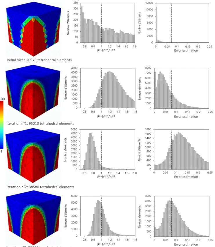
The adaptive procedure starts approximately with 21,000 uniformly distributed elements. A target error ~θoptel in the adap-tive process of 0.8% was adopted. The results are shown in Fig.6, where each line corresponds to a remeshing step taking the mesh in the previous line as the initial mesh. In practice, the elements size can’t respect perfectly the target error; hence, the sizes of elements can be very small or very large, especial-ly in the high gradient zones. The main cause of this non respect is the obligation to insert a midcap mesh in these zones in order to create a better evolution of the mesh size map. To evaluate the efficiency of the different used processes, global and local checks can be used: a first check is undertaken to simply calculate the average error of the new discretization. If this error is not close to the desired precision, it is certain that the built mesh is not optimal. However, even if the overall error is close to the desired one, this does not prove the opti-mality of new mesh. The main idea of the local check is to verify the error of the entire domainΩ for each element. In fact, if the element size is optimal, the procedure of successive adaptation must give change coefficients close to 1. According to [17], the size of the elements is considered sat-isfying in all areas with his modification size coefficient Re, where we have:
2=3≤Re≤3=2; Re¼ hnew=hold; ð41Þ
As shown in Fig.6, after each remeshing steps the density of element will increase or decrease in some zones in order to respect the target error. The evolution of the number of ele-ment in the histograms plot showed a concentration rise of elements numbers around the target error after each meshing step. For this analytic function five iterations can be consid-ered as satisfactory because the modification coefficients of element size Reis 90%, close to 1 in overall domain. In there-after examples this coefficients of element size criteria will be used in order to define the ideal number of iteration for each FEM problem.
Selection of the best recovery techniques
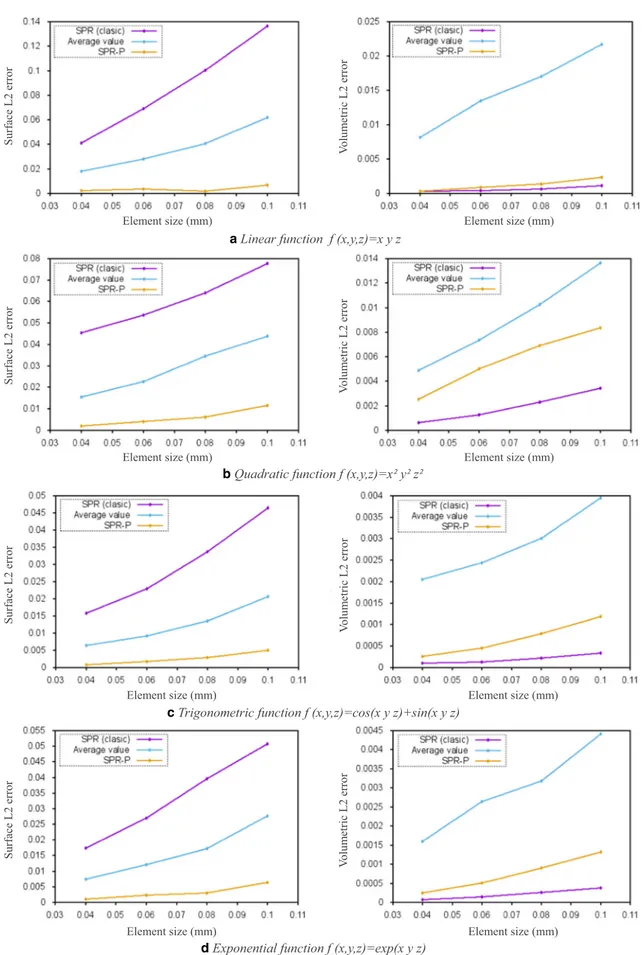
In order to select the best Patch Recovery Techniques to transfer the data state variables between two meshes, several analytical functions (linear and nonlinear) are considered in Fig.7. Here, we measure the exact error value, since the true solution is known. The approximated solution is made by using the smooth-ing techniques. The accuracy and convergence of each technique is examined with two different L2 error norms which are volu-metric norm Eq. (42) and surface norm Eq. (43). These L2 error norms measure the error between the recovered field values and the exact analytic solution.
ξ k kvol¼ ffiffiffiffiffiffiffiffiffiffiffiffiffiffiffiffiffiffiffiffiffiffiffiffiffiffiffiffiffiffiffiffiffiffiffiffiffiffiffiffiffiffiffiffiffiffiffiffiffiffiffiffiffiffiffiffiffiffi ∑k fk analyð Þ−fk SPR=SPR P=Avgð Þ ) ) ) ) ) ) 2 ∑k fk analyð Þ ) ) ) ) ) ) 2 v u u u u t ;∀k∈Ω ð42Þ ξ k ksurf ¼ ffiffiffiffiffiffiffiffiffiffiffiffiffiffiffiffiffiffiffiffiffiffiffiffiffiffiffiffiffiffiffiffiffiffiffiffiffiffiffiffiffiffiffiffiffiffiffiffiffiffiffiffiffiffiffiffiffiffiffi ∑k fk analyð Þ−fk SPR=SPR P=Avgð Þ ) ) ) ) ) )2 ∑k fk analyð Þ ) ) ) ) ) )2 v u u u u t ;∀k∈∂Ω ð43Þ
Figure 7 presents the volume and surface error values for SPR, SPR-P and Average recovery operator obtained for linear, quadratic, trigonometric and exponential func-tions for several meshes with uniformly decreasing element sizes. The corresponding comparison shows how the SPR technique values represent an improvement with respect to
Fig. 4 Two-dimensional superconvergent extended patch recovery (SPR-P)
100
1
the analytic values inside the domain, in comparison with the other techniques; but this improvement is not enough to ensure a good surface error prediction. This verdict is well known when the standard SPR technique is applied to boundary points, especially for coarse meshes. In order to
reduce the surface error booth, SPR-P and Average recov-ery technique can be used. Also, we can note that the error estimation both on surface and inside the domain illustrates better results with SPR-P recovery compared to the Average recovery technique.
1 100
Ini!al mesh 20973 tetrahedral elements
Itera!on n°2: 38580 tetrahedral elements
Itera!on n°5: 59000 tetrahedral elements Itera!on n°1: 95010 tetrahedral elements
Re=hnew/hold Error es!ma!on
Re=hnew/hold Error es!ma!on
Re=hnew/hold Error es!ma!on
Re=hnew/hold Error es!ma!on
a Linear function f (x,y,z)=x y z
b Quadratic function f (x,y,z)=x² y² z²
c Trigonometric function f (x,y,z)=cos(x y z)+sin(x y z)
d Exponential function f (x,y,z)=exp(x y z)
Element size (mm) Element size (mm)
Element size (mm) Element size (mm)
Element size (mm) Element size (mm)
Element size (mm) Element size (mm)
Surface L2 error Surface L2 error Surface L2 error Surface L2 error Vo lu m et ric L 2 er ro r Vo lu m et ric L 2 er ro r Vo lu m et ric L 2 er ro r Vo lu m et ric L 2 er ro r
For this work and in order to combine the advantage of these methods the SPR technique will be used to transfer the variables inside the domain and the SPR-P technique will be used to transfer the surface ones.
Adaptive REMESHING methodology
The proposed automatic adaptive remeshing strategy is pre-sented in Fig.8and tested by solving two numerical examples under large inelastic deformations and high strain localization. The purpose of these examples is to illustrate the efficiency of the adaptive remeshing scheme adopted to optimize the mesh according to the aimed prediction and to improve a good qual-ity of elements in each step-time. In this work and similar to [7], an element is classified as being distorted if one of his dihedral angles (angles between two faces) is larger than 160° or smaller than 10°, or if the radius-element ratio (the ratio between the volume of initial tetrahedron and the volume of
the regular tetrahedron registered in the same circumscribed ball, Fig.9) is smaller than 0.2.
Only for the first step, the initial finite elements discretization using a tetrahedral element is provided. Then, for each time step an ABAQUS 6.13/ Explicit FE calculation is performed with a small test displacement, and the resulting simulation is analyzed through a posteriori error estimators and element quality. If the estimated elementary error and / or the number of distorted elements does not exceed a given threshold, the previous FE simulation will be continued. Else, the mesh is then modified automatically (refined and / or coarsened) with MeshGems software according to the con-stantly changing physical fields and geometrical shape and a new solution for this loading sequence is computed. For each time step, this process is repeated many times until the mesh no longer changes and/or the error level has been reached. Finally, all field variables are transferred from the old mesh to the new one and the simulation is restarted from the previ-ous time step. It should also be noted that after each time step,
• Initialization of mechanical fields, t 0= 0s, iteration n = 0
• Definition of the geometry
• Definition of boundary conditions and material behavior
Small test displacement (Explicit)
Generation of the new mesh Mesh distortion
Or Error estimation
tn≤Ttotal
End
Transfer the thermomechanical fields between the old mesh and
the new mesh
Continue the previous FEM calculation Yes Yes No No Error estimation Small test displacement (Explicit) tn=tn+ ∆t tn=tn Yes No
Fig. 8 Flow chart of the FE-simulation for 3D remeshing module
the boundary and loading conditions are generated according to the old step modification.
Numerical results
Shear test
First, a shear test is used in order to validate the proposed methodology and study some numerical aspects. Then, a met-al forming process of a complex geometry will be tested. In each case, both the tool and the workpiece are discretized with tetrahedral elements C3D4T with thermomechanical coupling taken from ABAQUS element library. The mesh of the tools is selected before the first step and remains unchanged. However, the initial mesh of the work piece is a regular coarse mesh and will be automatically adapted during the FE process. In the adaptive process the smallest hminand largest hmax ele-ment sizes are respectively 0.1 mm and 1 mm. The contact interface between the tools and the parts is modelled by the classical Coulomb model with a constant friction coefficient
η = 0.2. Finally, material subroutine Vumat is implemented to predict the Johnson-Cook model [27] at each Gauss point for titanium alloy Ti17. The mechanical properties are similar to those reported in Reference [28].
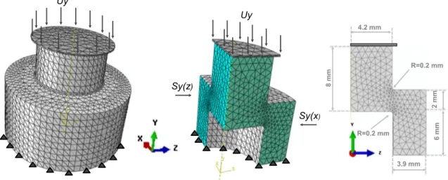
For the shear test, the geometry dimensions and boundary conditions are given in Fig.10. According to the symmetry conditions in a 3D configuration, only one quarter of the workpiece is modeled. To illustrate the efficiency of the adap-tive strategy under large inelastic deformations and high strain localization, two uniform displacements of the rigid tool has been analyzed. All the adaptive procedure starts with 2493 uniformly distributed elements (Fig.11a). Also, in order to attend the convergence of the FE solution and to study the influence of the element size on the stability of load, three target errors of 1%, 0.1%, and 0.03% have been used in the adaptive process. In this adaptive process, the smallest hmin
and largest hmax element sizes are 0.1 mm and 1 mm
respectively.
Fig.11b shows the final mesh obtained after four adaptive remeshing loops that can be compared with the initial one Fig.
11a. This adaptive remeshing loop is adopted at every time
Sy(z) Sy(x) Uy 8 mm 4.2 mm 3.9 mm R=0.2 mm 6 mm 2 m m Uy R=0.2 mm
Fig. 10 Geometry and boundary conditions of the specimens used in shear test
ini!al tetrahedron
circumscribed ball regular tetrahedron
Fig. 9 The radius-volume ratio of tetrahedron
step taking the adaptive deformed mesh in the previous step as the initial mesh. It can be observed how the adapted mesh concentrates additional elements in the critical zones whereas the number of elements in the rest of the domain remains practically unaltered or decreased.
We can note that the element size increases and the number of elements decreases with increasing the imposed target error. The comparison between the numerical load–displacement curves and published experimental data [28] with different deformation rate 1 mm/s and 100 mm/s are shown in Fig.
12. At Fig.12a, it can be shown that the smallest target error 0.03% is much more efficient in terms of convergence and accuracy of the FE solution in comparison with the large values 0.1 and 1%. However, even with this small target error 0.03% the system is not in mechanical equilibrium anymore. In fact, the numerical curves show a small fluctuation in the load-displacement response after each remeshing step which can be caused by a small degree of numerical diffusion during the transfer of variables between subsequent meshes. Also, we
can note that the level of fluctuation decreases with the de-cease of the target error used in the adaptive process. This non-smooth pattern fluctuation is also observed using various others approaches such as average values, closest point tech-nique [7], Superconvergent Patch Recovery (SPR) [22] or the unique element method (UEM) [29].
In Fig.12b, we consider the same shear test as previously presented in Fig.12a, but the shear test is performed under a high deformation rate of 100 mm/s. More fluctuation of load– displacement curves results under high deformation rate in comparison to the low one are observed.
Equilibrium process
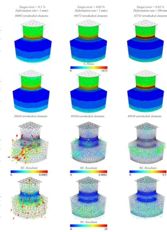
In order to solve the problem of this numerical instability, the results obtained before and after data transfer process between two successive meshes are compared. In Fig.13, the first line and the second one show the distribution of the von Mises stress components at integration points in each element; the
Fig. 12 Comparison of load–displacement curves of mechanical tests using different deformation rate: 1 mm/s and 100 mm/s Fig. 11 Meshes at different
instants with different targets errors
third line and the fourth one show the value of internal forces at tetrahedral element nodes Eq. (44).
fint ¼ fint x1 fint y1 fint z1 ⋮ fint xnnt fint ynnt fint znnt 2 6 6 6 6 6 6 6 6 6 4 3 7 7 7 7 7 7 7 7 7 5 ¼ ∫ VB T~σ dV; ð44Þ
where B is the spatial derivatives of the FE shape function.
The second line in Fig.13show a good continuous evolu-tion of the von Mises stress after the transfer, due to the stress smoothening. However, only with small target error test, very small smooth diffusion can be seen. Before meshing, the nod-al forces in the old mesh are very smnod-all since the explicit solver is used as shown in the third line and Eq. (45). However, it is not the case after remeshing specially in highly stain regions as shown in the fourth line. At this stage the main cause of the unbalanced system is due to the non-equilibrated forces at element nodes caused by stress smoothening in ele-ment. These nodal forces were self-equilibrated before trans-fer of state variables because the previous converged state was Target error = 0.1 % Target error = 0.03 % Target error = 0.03 % Deformation rate= 1 mm/s Deformation rate= 1 mm/s Deformation rate= 100 mm/s 30092 tetrahedral elements 94572 tetrahedral elements 82741 tetrahedral elements
30634 tetrahedral elements 88394 tetrahedral elements 80548 tetrahedral elements
0.0005 0. RF, Resultant 0.0001 0. RF, Resultant 0.5 0. RF, Resultant Aft er t ra nsf er (s te p5) Be fo re tra ns fer (s te p4 ) Af te r t ra ns fe r ( ste p5 ) B ef or e tr an sfe r ( st ep 4) 20 0. RF, Resultant 1473 0. S, Mises
Fig. 13 The evolution of the von Mises stress and the nodal force caused by stress smoothening before and after transfer at the same displacement u = 0.08 mm
valid only for the old mesh Eq. (45), but became external forces after transfer and are no longer in self-equilibrium with the new dynamic equilibrium equations Eq. (46).
div σel old ! "−mn old:γnold¼ 0 ð45Þ div σel new ! "−mn new:γnnew≠0; ð46Þ where σel
oldand σelneware respectively the initial and transferred
stress. mn old:γnold ! " and mn new:Ynnew ! "
are respectively the mass and acceleration of each node of the initial and finally mesh. From Figs.12 and13, it can be construed that if the rate deformation or the elements size used during the numeric simulation is sufficiently small, mechanical equilibrium can be established again at small time increment, because the transfer error is too small. In the case of high rate deformation, the remeshing process cannot be used because the numerical instability will be amplified (third row in Fig.13) even if the transfer error is too small.
So, to restore equilibrium with the new boundary condi-tions the unbalanced internal forces must be removed. However, if they are eliminated at once, often the following iterations are found in mechanical imbalance, especially for coarse meshes. Analogy example of Spring-mass system can be helpful to solve the equilibrium problem. In fact, when a
spring is stretched or compressed by a mass, the spring de-velops a restoring force. Only if this restoring force is small or relaxed the Spring-mass system can easily reach back to equi-librium. From this idea, a relaxation procedure has been im-plemented during the next step where these unbalanced nodal forces are removed successively by series of analytic function
Fig. 14 Comparison of load–displacement curves of mechanical tests before and after equilibrium
Fig. 15 Geometry, boundary conditions, and initial finite elements discretization
with decreasing coefficients. Note that only the values of dy-namic nodal force mnnew:γnneware kept. Where mnnewis the nodal
mass of the new mesh discretization and the new acceleration values at the nodal points γn
new are computed by an
interpolation of the old nodal acceleration via the FE shape function. The obtained results are presented in Fig.14.
It is obvious in Fig.14that the equilibrium recovery pro-posed in this work allows to restore equilibrium after each meshing step. In terms of convergence under high and low rate deformation, the computed load/displacement responses obtained with equilibrium process give a good approximation of the experimental solution compared to the one obtained by only direct transfer.
From these results, it can be concluded that the use of adaptive mesh process coupled with the proposed equilibrium recovery has the better results compared to the use of standard one, for which the equilibrium recovery process is not imposed.
Metal forming processes
The metal forging is simulated with Abaqus 6.13 software. The half of geometry and boundary conditions are shown in Fig.15. According to the symmetry conditions, only an eighth workpiece is modeled.
In order to demonstrate the interest and efficiency of adap-tive remeshing at a more complex geometries level, the same metal forging simulation is carried out with the presented mesh adaptation strategy (adaptive case) and without mesh adaptation (standard case). One of the critical ingredients in any FEM process is the mesh discretization. In fact, a severe mesh distortion can occur during the standard simulation es-pecially with constant coarse mesh. However, it is not the case with the adaptive test because the mesh is automatically adapted according to the constant change (physical fields and geometrical shapes). That’s why the initial mesh of the standard test must be optimized in some critical zones as shown in Fig.16. This comparison can improve a first advan-tage of using the adaptive process to avoid excessive mesh refinement, and present a good filling of the die matrices.
The numerical results presented in Fig.16show the effi-ciency of the adaptive remeshing process. In fact, from the beginning of the simulation to the end, a good quality of elements is proved with the adaptive strategy. However, a severe mesh distortion is observed without mesh adaptation. With the adaptive process, the simulation ends with zero ele-ment distortion compared to 6325 distorted eleele-ments without remeshing.
As it was noted above, each element size can be considered as optimal only if the procedures of successive mesh adapta-tion give modificaadapta-tion coefficient are close to 1. So, the remeshing iteration is repeated many times until the total num-ber of optimal elements does not exceed a given threshold. For this metal forging simulation, the target threshold of optimal elements number is selected as 75% and more strict area of modification coefficient is chosen 3/4≤ Re≤ 5/4 compared to
the reference coefficient proposed by Ladevèze [17] which is
2/3≤ Re≤ 3/2 Fig.17 shows that the both simulations start
with the same number of optimal elements. With the standard process, the percentage of optimal element decrease after each load displacement step until the end of simulation. In this stage, only 23% of elements are conformed to the target error. However, with the adaptive process if the percentage of opti-mal element is above the given threshold 75%, the previous FE simulation will be continued. Else, the mesh is then mod-ified automatically according to the constant change of phys-ical fields and geometrphys-ical shape. Another strong point of the presented process is that for each time step, the number of remeshing-iterations is not fixed, but it is automatically adapted, as shown in Fig.17. This characteristic can avoid the useless iteration and reduce time cost. For example for the first meshing step four iterations are performed; for the second and third meshing step two iterations; for the fourth meshing step only one iteration is used.
The evolution of numerical load–displacement curves with and without adaptive remeshing is compared in Fig.18. At the beginning of simulation both EF simulations give similar re-sults. However, it is not the case at the end of test. This
Fig. 18 Comparison of load–displacement curves of forming tests with and without mesh adaptation
Fig. 17 The evolution of the percentage of optimal element with and without mesh adaptation
difference may be caused by the presence of excessive mesh distortion in the standard test (without adaptive remeshing). As can be seen in Figs. 16and 19, these mesh distortions favors the displacement of elements in the second direction compared to the first one. In other words, the contact area between the rigid tool and the workpiece will not be the same especially in the second zone (II), which have a strongly effect on the normal load.
Conclusion
In this paper, an automatic adaptive remeshing method based on local mesh modification has been presented to simulate various 3D metal forming processes in large elastoplastic de-formations. This process has been implemented with a small test displacement step by step in order to adapt automatically to the constantly changing physical fields and geometrical shapes. At each time-step, the remeshing iteration is repeated many times until the total number of optimal elements does not exceed a given threshold. This characteristic can avoid the useless iteration and reduce time cost. To avoid numerical diffusion during the mapping of variables, data transfer error is examined using analytical functions such as linear, quadrat-ic, trigonometric and exponential with volumetric L2 error norms and surface one. The results show that these techniques illustrate different efficiency. So, in order to combine the ad-vantage of these methods the SPR technique will be used to transfer the variables inside the domain and the SPR-P tech-nique will be used to transfer the surface ones. Without equil-ibrate process, the numerical load-displacement curves under large displacement and/or high deformation rate show that after each remeshing step the system is not in mechanical equilibrium anymore. In fact, the numerical curves show a small fluctuation in the load-displacement response after each remeshing step. But with the proposed equilibrated process a good agreement with experimental data has been observed and the imbalance fluctuations are reduced significantly.
Also, a good quality of elements is proven with the adaptive strategy, where a severe mesh distortion is observed without mesh adaptation which can significantly reduce the efficiency of numerical result. Finally, the overall results are very encour-aging and show the efficiency and robustness of the proposed strategy to avoid mesh distortion and to simulate more com-plex geometry levels with a better filling of the die matrices compared to the standard approach. However, several points can be improved such as damage evolution.
References
1. Diez P, Calderon G (2007) Remeshing criteria and proper error representations for goal oriented h-adaptivity. Comput Methods Appl Mech Engrg 196(4-6):719–733
2. Ainsworth M, Oden JT (1997) A posteriori error estimation in finite element analysis. Comput Methods Appl Mech Engrg 142(1-2):1– 88
3. Verfurth R (1999) A review of a posteriori error estimation tech-niques for elasticity problems. Comput Methods Appl Mech Engrg 176(1-4):419–440
4. Lo SH (1991) Volume discretization into tetrahedra-1. Verification and orientation of boundary surfaces. Comput Struct 39(5):493– 500
5. Lo SH (1991) Volume discretization into tetrahedra-II. 3D triangu-lation by advancing front approach. Comput Struct 39(5):501–511 6. Dureisseix D, Bavestrello H (2006) Information transfer between incompatible finite element meshes: application to coupled thermo-viscoelasticity. Comput Methods Appl Mech Engrg 85:6523–6541 7. Zeramdini B, Robert C, Germain G, Pottier T (2016) Simulation of metal forming processes with a 3D adaptive remeshing procedure. AIP Conf Proceed.https://doi.org/10.1063/1.4963636
8. Srikanth A, Zabaras N (2000) Shape optimization and preform design in metal forming processes. Comput Methods Appl Mech Engrg 190(13–14):1859–1901
9. Kumar S, Fourment L, Guerdoux S (2015) Parallel, second-order and consistent remeshing transfer operators for evolving meshes Fig. 19 The effect of mesh-distortion on the geometry of the workpiece
with superconvergence property on surface and volume. Finite Elem Anal Des 93:70–84
10. Peric D, Hochard C, Dutko M, Owen DRJ (1996) Transfer opera-tors for evolving meshes in small strain elasto-placticity. Comput Methods Appl Mech Engrg 137(3-4):331–344
11. Zienkiewicz OC, Zhu JZ (1992) The superconvergent patch recov-ery (SPR) and adaptive finite element. Comput Methods Appl Mech Engrg 101(1-3):207–224
12. Zienkiewicz OC, Zhu JZ (1992) The superconvergent patch recov-ery and a posteriori error estimation. Part I: the recovrecov-ery technique. Internat J Numer Methods Engrg 33(7):1331–1364
13. Zienkiewicz OC, Zhu JZ (1992) The superconvergent patch recov-ery and a posteriori error estimation. Part II: error estimates and adaptivity. Internat J Numer Methods Engrg 33(7):1365–1382 14. Babuška I, Rheinbildt WC (1978) A posteriori error estimates for
the finite element method. Internat J Numer Methods Engrg 12(10): 1597–1615
15. Ladevèze P, Coffignal G, Pelle J.P (1986) Accuracy of elastoplastic and dynamic analysis. In Babuška I, Zienkiewicz O.C, Gago J and Oliveira E.R de A, ch.11 Accuracy Estimates and Adaptive Refinements in Finite Element Computations, John Wiley & Sons Ltd pp 181–203
16. Zienkiewicz OC, Zhu JZ (1987) A simple error estimator and adap-tive procedure for practical engineering analysis. Int J Numer Methods Eng 24(2):337–357
17. Ladevèze P, Pelle J.P (2004) Mastering calculation in linear and nonlinear mechanics, Berlin
18. Boussetta R, Fourment L (2004) A posteriori error estimation and three-dimensional adaptive remeshing: application to error control of non-steady metal forming simulations. AIP Conf Proc 712: 2246–2251
19. Boussetta R, Coupez T, Fourment L (2006) Adaptive remeshing based on a posteriori error estimation for forging simulation. Comput Methods Appl Mech Engrg 195(48-49):6626–6645
20. Coorevits P, Bellenger E (2004) Alternative mesh optimality criteria for h-adaptive finite element method. Finite Elem Anal Des 40: 2195–1215
21. Ciarlet P.G (1978) The finite element method for elliptic problems. North-Holland publishing company, Amsterdam, New York, 45, 4 22. Khoei AR, Gharehbaghi SA, Tabarraie AR, Riahi A (2007) Error estimation, adaptivity and data transfer in enriched plasticity con-tinua to analysis of shear band localization. Appl Math Model 31(6):983–1000
23. Babuška I, Strouboulis T, Upadhyay CS, Gangaraj SK, Copps K (1994) Validation of a posteriori error estimators by numerical ap-proach. Int J Numer Methods Engrg 37(7):1073–1123
24. Wiberg NE, Abdulwahab F, Ziukas S (1994) Enhanced superconvergent patch recovery incorporating equilibrium and boundary conditions. Inter J for Numer Methods Engrg 37(20): 3417–3440
25. Liszka T, Orkisz J (1980) The finite differences method at arbitrary irregular grids and its application in applied machanics. Comput Struct 11(1-2):83–95
26. Liszka T (1984) An interpolation method for an irregular net of nodes. Int J Numer Methods Engrg 20(9):1599–1612
27. Johnson G.R, Cook W.K (1983) A constitutive model and data for metals subjected to large strains high strain rates and high temper-atures. 7th international symposium on Balistics pp 541–547 28. Ayed Y, Germain G, Ammar A, Furet B (2016) Thermo-mechanical
characterization of the Ti17 titanium alloy under extreme loading conditions. Int J Adv Manuf Technol 90:5–8.https://doi.org/10. 1007/s00170-016-9476-5
29. Hu Y, Randolph MF (1998) H-adaptive FE analysis of elasto-plastic non-homogeneous soil with large deformation. Comput Geotech 23(1-2):61–83