Is it time to revisit Erasure Coding in Data-intensive clusters?

HAL Id: hal-02263116

https://hal.inria.fr/hal-02263116

Submitted on 2 Aug 2019

HAL is a multi-disciplinary open access

archive for the deposit and dissemination of

sci-entific research documents, whether they are

pub-lished or not. The documents may come from

teaching and research institutions in France or

abroad, or from public or private research centers.

L’archive ouverte pluridisciplinaire HAL, est

destinée au dépôt et à la diffusion de documents

scientifiques de niveau recherche, publiés ou non,

émanant des établissements d’enseignement et de

recherche français ou étrangers, des laboratoires

publics ou privés.

Is it time to revisit Erasure Coding in Data-intensive

clusters?

Jad Darrous, Shadi Ibrahim, Christian Pérez

To cite this version:

Jad Darrous, Shadi Ibrahim, Christian Pérez. Is it time to revisit Erasure Coding in Data-intensive

clusters?. MASCOTS 2019 - 27th IEEE International Symposium on the Modeling, Analysis, and

Simulation of Computer and Telecommunication Systems, Oct 2019, Rennes, France. pp.165-178,

�10.1109/MASCOTS.2019.00026�. �hal-02263116�

Is it time to revisit Erasure Coding in

Data-intensive clusters?

Jad Darrous

Lyon, France jad.darrous@inria.fr

Shadi Ibrahim

Nantes, France shadi.ibrahim@inria.fr

Christian Perez

Lyon, France christian.perez@inria.fr

Abstract—Data-intensive clusters are heavily relying on dis-tributed storage systems to accommodate the unprecedented growth of data. Hadoop distributed file system (HDFS) is the primary storage for data analytic frameworks such as Spark and Hadoop. Traditionally, HDFS operates under replication to ensure data availability and to allow locality-aware task execution of data-intensive applications. Recently, erasure coding (EC) is emerging as an alternative method to replication in storage systems due to the continuous reduction in its computation over-head. In this work, we conduct an extensive experimental study to understand the performance of data-intensive applications under replication and EC. We use representative benchmarks on the Grid’5000 testbed to evaluate how analytic workloads, data persistency, failures, the back-end storage devices, and the network configuration impact their performances. Our study sheds the light not only on the potential benefits of erasure coding in data-intensive clusters but also on the aspects that may help to realize it effectively.

Index Terms—Erasure codes, Hadoop, MapReduce, Experi-mental evaluation, Data-intensive clusters.

I. INTRODUCTION

With the increasing amount of generated data and the necessity for efficiently managing it, many Distributed File Systems (DFSs) have been developed [22], [50]. These sys-tems rely on thousands of commodity machines to store the data. At such scale, machine failure is the norm rather than the exception [22], and thus, file systems should handle failures gracefully. To ensure data availability and durability, files are usually replicated on multiple machines. Current data analytic frameworks (e.g., Hadoop [6], Spark [7], etc) – that rely on the principle of moving computation to data – have extensively explored the benefits of data replication to improve the performance of data-intensive applications by increasing the data locality of running (map) tasks [18], [29], [56]. That is, if a machine holding the input data of a task is not available (i.e., computation resources are occupied running other tasks), the task can be run on another machine which has a replica of the same data. However, with the relentless growth of Big Data, and the wide adoption of high-speed yet expensive storage devices (i.e., SSDs and DRAMs) in storage systems, replication (REP) has become expensive [43], [47], [60] in terms of storage cost and hardware cost. Therefore, new techniques have been introduced such as relying on one

active replica [42] or using erasure coding (EC) techniques [2], [8], [26].

Erasure coding is a method which can provide the same fault tolerance guarantee as replication [46] while reducing storage cost. However, EC reduces storage cost in exchange for more computation, disk, and network overhead; encoding and de-coding are considered CPU intensive operations, furthermore, reconstructing missing blocks may require a considerable amount of data to be read and transferred over the network (usually many times the size of the block). Thus, EC has been mainly employed to store archived data in peer-to-peer systems [32], [46] and cold data [23], [40]; such data that are not frequently accessed.

Recently, important progress has been made in reducing the CPU overhead of EC operations. Intel Intelligent Storage Acceleration Library (ISA-L) [10] has been released with EC operations, among others, implemented and run at CPU speed (e.g., encoding throughput using only one single core is 5.3 GB/s for Intel Xeon Processor E5-2650 v4 [4]). This allows the integration of EC operations on the critical path of data accesses [44]. As a result, EC has been employed in in-memory storage systems on cached (hot) data [44], [58] and is integrated in the last major release of Hadoop Distributed File System (i.e., HDFS 3.0.0) which is the primary storage back-end for data analytics frameworks (e.g., Hadoop [6], Spark [7], Flink [5], etc).

Given that data processing applications have become first-class citizens in many industrial and scientific clusters, in this work, we aim to answer a broad question: How erasure coding performs compared to replication for data processing appli-cations in data-intensive clusters?The explosion of Big Data, the recent advances in storage devices, and the emergence of high-speed network appliances [11], [13] elevate EC as an ideal candidate to replace replication in data-intensive clusters. Previous efforts to explore EC for data-intensive applica-tions have applied EC with contiguous data layout (i.e., "n" HDFS blocks are used to generate "k" parity blocks) to in-crease the probability of local map task executions (i.e., realize disk locality) [34]–[36], [59]. However, EC with contiguous data layout may not be practical in production clusters due to its high memory overhead when encoding data and for its inefficiency for handling small files [59], [60]. The current

efforts on adopting EC in HDFS acknowledge this limitation and therefore applied EC with striped data layout (i.e., HDFS block is represented by "n" original chunks and "k" parity chunks) in current release of Hadoop (i.e., Hadoop 3.0.0) [6], [60].

In this work, we focus on EC with striped data layout and provide – to the best of our knowledge – the first study on the impact of EC with striped data layout on the task runtimes and application performances. Accordingly, we con-duct experiments to thoroughly understand the performance of data-intensive applications under replication and EC. We use representative benchmarks on the Grid’5000 [9] testbed to evaluate how analytic workloads, data persistency, failures, the back-end storage devices, and the network configuration impact their performances. While some of our results follow our intuition, others were unexpected. For example, disk and network contentions caused by chunks distribution and the unawareness of their functionalities are the main factor affecting the performance of data-intensive applications under EC, not data locality.

An important outcome of our study is that it illustrates in practice the potential benefits of using EC in data-intensive clusters, not only in reducing the storage cost – which is becoming more critical with the wide adoption of high-speed storage devices and the explosion of generated and to be processed data – but also in improving the performance of data-intensive applications. For example, in the case of Sort application, although EC requires most of the input data to be transferred during the map phase, the performance of map tasks degraded by 30% on average under EC. But, given that the output data is relatively large which is common in many scientific data-intensive applications1_{, reduce tasks finish much}

faster – and thus earlier – under EC compared to replication. As a result, although EC introduces higher network overhead (almost 8%) compared to replication, EC achieves an overall performance improvement of up to 25%. We hope that the insights drawn from this paper will enable a better understand-ing of the performance of data-intensive applications under EC and motivate further research in adopting and optimizing EC in data-intensive clusters.

Applicability. It is important to note that the work (and the findings) we present here neither is limited to HDFS implementation nor specific to Hadoop MapReduce and can be applied to other distributed file systems that implement a striped layout erasure coding policy. Moreover, our find-ings can be valid with other data analytic frameworks (e.g., Spark [7], Flink [5], etc) if they run on top of HDFS as the impact of EC will be for reading the input data and writing the output data; not on how the actual computation and task scheduling are performed.

The remainder of this paper is organized as follows. Sec-tion II introduces Hadoop framework and Erasure Codes, followed by the related work in Section III. The

experi-1_{Analysis of traces from production "Web Mining" Hadoop cluster [3]) reveals that}

the size of output data is at least 53% of the size of input data for 96% of web mining applications.

mental methodology is explained in Section IV. Section V and Section VI present the different sets of experiments highlighting the impact of erasure coding on the performance of MapReduce applications and summarize our observations. Section VII discusses guidelines and new ways to improve data analytics under erasure coding. Finally, Section VIII concludes this study.

II. BACKGROUND

A. Apache Hadoop

Apache Hadoop [6] is the de-facto system for large-scale data processing in enterprises and cloud environment. Hadoop MapReduce framework is an implementation of the MapRe-duce programming model that has been originally introMapRe-duced by Google [18], [30].

Hadoop MapReduce jobs run on top of Hadoop Distributed File System (HDFS) [50]. HDFS is inspired by Google File System (GFS) [22] which is designed to store multi-gigabytes files on large-scale clusters of commodity machines. There-fore, HDFS is optimized for accessing “large” files. This is achieved by relaxing the POSIX interface (e.g., random write inside a file is not supported). To ease the management of its data, files stored in HDFS are divided into blocks, typically with a size of 64 MB, 128 MB, 256 MB, etc. To ensure data availability in case of failures, each block is replicated on three different machines, with one replica in another rack. HDFS consists of a NameNode and a set of DataNodes. The NameNode (NN) process is responsible for mapping each file to a list of blocks and maintains the distribution of blocks over the DataNodes. The DataNode (DN), on the other hand, manages the actual data on its corresponding machine.

YARN [51] is the resource manager of Hadoop system. It is responsible for allocating containers that run the map and reduce tasks. It has a master process (i.e., ResourceManager (RM)) and a process for each running application (i.e., Ap-plicationManager). Each worker node runs a NodeManager (NM) process.

B. Erasure Codes

Erasure coding is an encoding technique which can provide the same fault tolerance guarantee as replication [46] while reducing storage cost.

Reed-Solomon codes (RS) [45] are the most deployed codes in current storage systems [2], [21], [50]. RS(n, k) splits the block of the data to be encoded into (n) smaller blocks called data chunks, and then computes (k) parity chunks from these data chunks. In this paper, a block refers to the original data block (i.e., HDFS block of 256 MB). This block is represented as n original chunks and k parity chunks. The collection of (n + k) chunks is called a stripe, where n + k is the stripe width. In a system deploying an RS code, the (n + k) chunks belonging to a stripe are stored on distinct failure domains (e.g., disks, machines, racks, etc) in order to maximize diversity and tolerate maximum resource unavailability.

RS codes have the property of Maximum Separable

Dis-tance [38], which means that any (n) out of (n + k) is

sufficient to rebuild the original data block, thus, RS codes can tolerate (k) simultaneous failures. RS codes present a trade-off between higher fault tolerance and lower storage overhead depending on the parameters (n) and (k). RS(6, 3) and RS(10, 4) are among the most widely used configurations. Compared to replication, RS(6, 3) has a storage overhead of 50% and delivers the same fault-tolerance (i.e., tolerating 3 simultaneous failures) as 4-way replication that incurs a storage overhead of 300%.

On the other hand, in addition to CPU overhead, EC bring considerable network and disk overhead in case of failure (i.e., data loss). In particular, to reconstruct a missing chunk, n chunks (original and/or parity) should be read (from disk) and transferred over the network. Therefore, the reconstruction cost of a chunk is n times its size in terms of (network) data transfer and (disk) read. While for replication, to recover a missing piece of data, the amount of data which is read and transferred is equal to the size of the missing data, and has a negligible CPU overhead.

C. Block layout in HDFS

The mapping between logical blocks and the physical ones can be either contiguous or striped. For contiguous block layout, each physical block represents a logical block, while for striped layout, one logical block is represented physically by multiple chunks – usually distributed on multiple disks.

It is important to note that the block layout is orthogonal to the redundancy strategy (i.e., EC or REP). For example, in HDFS, the contiguous block layout is used for replication, while the striped one is employed in case of erasure coding. The reason behind using contiguous block layout in case of replication is simply to eliminate the need for any network transfer in case of local task executions as the complete data of the block can be read sequentially from one machine. However, EC is implemented using striped block layout – in HDFS version 3.0.0 and later releases – for two main reasons; first, it is more efficient for small files i.e., files with less than (n) blocks. For example, in case of RS(6, 3), a file with a size of one HDFS block will incur a 300% storage overhead [60], under contiguous block layout, as three parity blocks will still be needed. Second, encoding and decoding require less memory overhead; for contiguous layout, the complete n blocks should be available in the machine’s main memory for encoding and decoding (e.g., 9 ∗ 256 MB should be available in memory at the same time for encoding and decoding), while these operations are done on the cell level with a striped layout, thus only 9 ∗ 1 MB is required in the memory for encoding and decoding. Nevertheless, currently, there is a work in progress to design EC with contiguous layout2 _{in HDFS.}

Storing a block in HDFS under EC (with striped block layout) imposes higher metadata overhead at the NameNode.

2_{WIP https://issues.apache.org/jira/browse/HDFS-8030}

Under EC, a block is distributed to n + k nodes (under RS(n, k)), while under replication, a block is stored on 3 nodes. Therefore, in order to reduce the metadata overhead, under RS(n, k), every n blocks – belonging to the same file – are grouped into an EC group. Accordingly, all the blocks of the same EC group are placed on the same set of nodes. To encode this group of blocks, the blocks are encoded sequentially. Each block is split into cells (e.g., 1 MB), then the client encodes each n cells to generate k parity cells. The client sends these n + k cells to the n + k DNs, and then continues to do the same with the remaining cells, and repeats the same process for the remaining blocks in the group. On the other hand, data blocks (i.e., original chunks) can be read in parallel from multiple DNs. This parallelization can achieve better performance especially when the network bandwidth is higher than the disk bandwidth [12].

III. RELATEDWORK

Many research efforts have been dedicated to adopt erasure coding in data-intensive clusters [2], [20]. HDFS-RAID [2] and DiskReduce [20] extend HDFS to encode replicated data offline. The blocks are initially replicated and periodic MapReduce jobs are launched later to identify cold blocks and encode them asynchronously. Some recent works focus on online encoding (i.e., the data is encoded once it is written to HDFS) and study the performance of MapReduce applications. Zhang et al. [59] implement EC with a contiguous layout on the top of HDFS on the critical path. They show that the execution times of MapReduce applications can be reduced when intermediate data and output data are encoded compared to 3-ways replication. This is due to the reduction in the amount of data which is written to disk and transferred through the network. Our work is different as we focus on EC with a striped layout. In addition, they assume that map tasks are all executed locally under EC and no data transfer occurs during the map phase which is not realistic in practice. Non-systematic codes like Carousel [34] and Galloper [35] codes have been introduced to improve data locality under EC. In-stead of distributing the original data chunks and parity chunks on distinct nodes and thus nodes which host parity chunks cannot execute map tasks locally, parity data are appended to original blocks and thus all the DataNodes host both original data and parity data. Runhui et al. [36] propose degraded-first scheduling to improve the performance of MapReduce applications under failure. They focus on task scheduling in case of failures for map tasks that may require degraded reads for their input data (i.e., read is degraded when the required block is not available and thus should be reconstructed on the fly by retrieving other data and parity blocks). This will block the execution of map tasks and prolong the execution time of MapReduce applications. To address this issue, degraded tasks are scheduled earlier when network resources are not fully used.

Although important, the aforementioned studies do not provide a comprehensive picture of how data-intensive appli-cations perform under erasure coding. In contrast, we consider

different data-intensive applications (with different character-istics and job sizes) and different system configuration (HDD, SSD, DRAM, 1 Gbps and 10 Gbps network, etc) and provide the first in-depth study of the impact of EC with striped data layouton the task runtimes and application performances. This can help researchers to identify the challenges and therefore provide adequate solutions accordingly.

IV. METHODOLOGYOVERVIEW

We conducted a set of experiments to assess the impact of analytic workloads, data persistency, failures, the back-end storage devices, and the network configuration on the per-formance of data-intensive applications when HDFS operates under replication (REP) and erasure coding (EC).

Platform. We have performed our experiments on top of Hadoop MapReduce 3.0.0. We evaluate MapReduce appli-cations in two scenarios: when overlapping map phase and shuffle stage in reduce phase – as in Hadoop MapReduce and Flink – and when there is no overlapping between the two phases – as in Spark [48], [57].

Testbed. Our experiments were conducted on the French scientific testbed Grid’5000 [9] at the site of Nantes. We used for our experiments the Econome cluster, which comprises 21 machines. Each machine is equipped with two Intel Xeon E5-2660 8-cores processors, 64 GB of main memory, and one disk drive (HDD) at 7.2k RPM with 1 TB. The machines are connected by 10 Gbps Ethernet network, and run 64-bit Debian stretch Linux with Java 8 and Hadoop 3.0.0 installed. All the experiments have been done in isolation on the testbed, with no interference originated from other users.

In all the experiments, one node is dedicated to run the NameNode and the ResourceManager, while the remaining 20 nodes serve as workers (i.e., DataNodes and NodeManagers). Network bandwidth of 1 Gbps links is emulated with the Linux Traffic-Control tool [1].

Hadoop configuration. HDFS block size is set to 256 MB and the replication factor is set to 3. For EC, if not otherwise stated, we use the default EC policy in HDFS, i.e., RS(6, 3) scheme with a cell size of 1 MB. We disable speculative execution to have more control over the number of launched tasks. We configure YARN to run 8 containers per node (i.e., one per CPU core). Therefore, 160 slots are available in our cluster, which is sufficient to process 40 GB of data in a single map wave.

Benchmarks. We evaluate the performance of MapReduce with two micro-benchmarks (i.e., Wordcount and Sort) and one iterative application (i.e., Kmeans). Wordcount application is considered map intensive with small output size, which accounts for the majority of jobs in production data-intensive clusters (e.g., about 70% of the jobs in Facebook clusters [16]). Sort application is considered shuffle intensive and generates an output equal in size to the input, which represents a big portion of scientific and production applications (e.g., traces collected at Cloudera show that, on average, 34% of jobs across five customers had output at least as large as

their inputs [16]). Both Wordcount and Sort applications are available with Hadoop distribution.

In addition to the micro-benchmarks, we evaluated Kmeans application from the HiBench suite [27]. Kmeans is a basic Machine Learning application that is used to cluster multi-dimensional datasets. We used the provided synthetic dataset generator of HiBench to generate a dataset with 1200M samples of 20 dimensions each, which results in a total size of 222 GB. We set the number of clusters to 5 and set the maximum number of iterations to 10.

Each job is running alone, thus, it has all the resources of the cluster during the execution. We run each experiment 5 times and we report the average alongside the standard deviation. Moreover, when analyzing a single run we present the results of the job with the median execution time. We cleared the caches between data generation and data processing, as well as between the runs.

Metrics. We used the execution time and the amount of

exchanged data for MapReduce applications; Job execution

time is the total time of the job from its start time to finish time (not including time waiting in the queue). Exchanged data is the amount of data that goes over the network between the DNs. It consists of non-local read for input data, the shuffled data, and the non-local write of output data. It is measured as the difference between the bytes that go through each machine network interface, for all the DNs, before and after each run. Also, we used the coefficient of variation metric to measure the variation in tasks’ (map and reduce) runtimes.

During all the experiments, we collect the metrics related to CPU utilization, memory utilization, disk, and network I/O of the DataNodes using the python library psutil3_.

V. DATA PROCESSINGUNDEREC

A MapReduce job consists of two phases: (1) map phase: map tasks read the input data from HDFS and then write the intermediate data (i.e., the output of the map phase/input for the reduce phase) in the local disks after applying the map function. (2) reduce phase which in turn includes three stages: shuffle stage which can be performed in parallel with map phase, sort stage and finally reduce stage. Sort and reduce stages can only be performed after the map phase is completed. In the reduce stage, data are written to HDFS after applying the reduce function. However, we note here that writing data to HDFS is considered successful when the data is completely buffered in the memory. Consequently, a job can be considered as finished before all the output data are persisted to disks. When running MapReduce applications, HDFS is accessed during the map phase and the reduce stage, whereas, intermediate data is written to the local file system of the DNs.

A. Hadoop when NO overlapping between the map and reduce phases

To facilitate the analysis of MapReduce jobs and focus on the differences regarding REP and EC (i.e., reading input

10 20 40 80 Input data size (GB) 0 50 100 150 200 250 Time (sec)

(a) Sort execution time

10 20 40 80 Input data size (GB) 0 20 40 60 80 100 120 140 160 Time (sec)

(b) Wordcount execution time Fig. 1. Job execution time of Sort and Wordcount MapReduce applications under EC and REP (non-overlapping shuffle).

TABLE I

DETAILED EXECUTION TIMES OFSORT ANDWORDCOUNTMAPREDUCE APPLICATIONS FOR40 GBINPUT SIZE IN SECOND WITH THE PERCENTAGE

OF EACH PHASE.

Job execution time Map Phase Reduce Phase

Sort EC 113.6 70.6 (64.2%) 38.3 (35.8%)

REP 103.9 43.4 (43.9%) 54.3 (56.1%)

Wordcount EC 113.7 101 (90.8%) 8.2 (9.2%)

REP 73.8 60.4 (85%) 8.4 (15%)

data and writing output data) we start with the case when there is no overlapping between the map phase and the reduce phase (during the shuffle). The same approach is employed in Spark. While, in MapReduce, the shuffle starts when a specific number of map tasks finish (5% by default). This allows the overlapping between the computation of map tasks and the transfer of intermediate data.

First, the job execution time of Sort application while increasing input sizes is depicted in Fig. 1a. We can notice that REP slightly outperforms EC. For 40 GB input size (as stated before, we focus on the run with the median job execution time), job execution time under EC is 113.6s, thus 9% higher than that under REP (103.9s). This difference can be explained by the time taken by the map and reduce phases (as shown in Table I), knowing that these two phases are not overlapping. Map phase finishes faster under REP by 38% (70.6s under EC and 43.4s under REP). On the other hand, reduce phase finishes faster under EC compared to REP by 29% (38.3s under EC and 54.3s under REP).

Runtimes distribution of map and reduce tasks. Fig. 2 shows the timeline of task runtimes under both EC and REP. We can clearly see that the main contributor to the increase in the runtimes of reduce tasks under REP compared to EC is reduce stage, in particular, writing data to HDFS. While the times of shuffle and sort stages are almost the same under both EC and REP, REP needs more time to transfer the output data to the DNs: 53.3 GB under EC, among which 10.2 GB are written to disks, while 80 GB are transferred through network to DNs under REP, among which 32.8 GB are persisted to disks. The remaining are buffered in OS caches. On the other hand, we can see high variation in the runtimes of map tasks under EC compared to REP. Map runtime varies by 33.3% under EC (from 7.9s to 69.2s) while it varies by 15.8% under REP (from 13.7s to 43.2s) and the average runtimes are 38.6s

0 10 20 30 40 50 60 70 80 90 100 110 120 Timestep 0 25 50 75 100 125 150 175 200

Map tasks Shuffle stage Sort stage Reduce stage

(a) REP 0 10 20 30 40 50 60 70 80 90 100 110 120 Timestep 0 25 50 75 100 125 150 175 200

Map tasks Shuffle stage Sort stage Reduce stage

(b) EC

Fig. 2. Tasks of Sort MapReduce application under EC and REP

(non-overlapping shuffle) for 40 GB input size. The first 160 tasks are map tasks, while the remaining 36 tasks are reduce tasks.

EC REP 0 1 2 3 4 5 6 7 8 Data size (GB)

(a) Initial data distri-bution (NO) EC REP 0.0 0.5 1.0 1.5 2.0 2.5 3.0 3.5 Data size (GB)

(b) Data read per ma-chine (NO) EC REP 3 4 5 6 7 8 Data size (GB)

(c) Write load distri-bution (O)

Fig. 3. Initial data load on DNs, data read per node, and data written per node for non-overlapping (NO) and overlapping (O) cases.

and 29.6s under EC and REP, respectively. Interestingly, we find that the minimum runtime of map tasks under EC is 7.9s while it is 13.7s under REP. Moreover, the runtimes of 25% of map tasks under EC are below the average of map runtimes under REP. Hence, the degradation in the runtimes of map tasks under EC is not due to data locality or network overhead, especially as the network is under-utilized during the whole map phase under EC (100 MB/s on average).

Zoom-in on map phase. Fig. 3a shows the distribution of input data. We notice that the variation in data distribution is almost the same under both EC and REP (a standard deviation of 1.36 GB under EC and 1.13 GB under REP). Accordingly, and given that each node executes the same number of map tasks, we expect that the amount of data read by each node is the same: as we run 8 containers per node, and each map task handles 1 block of data (256 MB), therefore, ideally 2 GB of data should be read by each DN. However, as shown in Fig. 3b, the amount of data read varies across nodes under both REP and EC. Under REP, we can see this with a couple

0 10 20 30 40 50 60 70 80 90 100 110 120 Timestep 0 25 50 75 100 125 150 175 200

Map tasks Shuffle stage Sort stage Reduce stage

(a) REP 0 10 20 30 40 50 60 70 80 90 100 110 120 Timestep 0 25 50 75 100 125 150 175 200

Map tasks Shuffle stage Sort stage Reduce stage

(b) EC

Fig. 4. Tasks of Wordcount MapReduce application under EC and REP (non-overlapping shuffle) for 40 GB input size. The first 160 tasks are map tasks, while the remaining 36 tasks are reduce tasks.

of outliers that represent non-local reads (in our experiments, the achieved data locality is 94%); hence this contributes to the variation in the map runtimes under REP. On the other hand, we observe high variation (44.3%) in the data read across DNs under EC. This imbalance of data read under EC is related to the fact that HDFS block distribution algorithm does not distinguish between an original chunk and a parity chunk under EC, thus, some DNs might end up with more parity chunks than others even though they have the same total number of chunks. As map tasks do not read parity chunks when there is no failure or data corruption, the imbalance in data read occurs and results in longer runtimes of map tasks. Nodes which are continuously serving map tasks running in other nodes will exhibit high CPU iowait time and therefore the runtimes of map tasks running within them will increase. The median iowait time of the node with the largest data read (3.53 GB) is 82% while the median iowait time of the node with the lowest data read (0.35 GB) is 0.7%. Consequently, the average of map runtimes (map tasks running within the two aforementioned nodes) is 59s and 25s, respectively. As a result, the runtimes of map tasks which are severed by those nodes will also increase. In conclusion, Hadoop exhibits high read imbalance under EC which causes stragglers. This, in turn, prolongs the runtimes of map tasks compared to REP and causes high variation in map runtimes.

The same trend can be observed with Wordcount application (where the shuffle data and final output are relatively small compared to the input size); Load imbalance in data read across nodes under EC which results in longer (and high variation in) map runtimes (CPU iowait during the map phase is around 15% under EC and almost zero under REP). However, as the job execution time (shown in Fig. 1b) is

10 20 40 80 Input data size (GB) 0 50 100 150 200 250

Exchanged data siz

e (GB)

(a) Sort application

10 20 40 80 Input data size (GB) 0

20 40 60 80

Exchanged data siz

e (GB)

(b) Wordcount application

Fig. 5. Amount of exchanged data between DataNodes during the job

execution (non-overlapping shuffle).

10 20 40 80

ECREP ECREP ECREP ECREP

Data size (GB) 0 50 100 150 200 250 300 Time (sec)

(a) Sort execution time

10 20 40 80

ECREP ECREP ECREP ECREP

Data size (GB) 0 20 40 60 80 100 120 140 160 Time (sec)

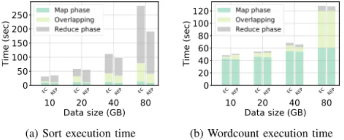
(b) Wordcount execution time Fig. 6. Job execution time of Sort and Wordcount MapReduce applications under EC and REP.

dominated by the map phase (as shown in Table I and Fig. 4, the map phase accounts for around 90% of the execution time for Wordcount application), and given that map phase is quicker by 40% under REP (101s under EC and 60.4s under REP); Wordcount application finishes 35% slower under EC compared to REP (the job execution time is 113.7s and 73.8s under EC and REP, respectively). Note that reduce phase takes almost the same time under both EC and REP (8.2s and 8.4s, respectively) as the final output data is relatively small.

Finally, Fig. 5a and Fig. 5b show the amount of transferred data between the DNs when running Sort and Wordcount applications with different input sizes, respectively. When sorting 40 GB input size, 137 GB is transferred under EC, 8.7% more than that under REP (125 GB). However, for Wordcount application, 10x more data are transferred under EC. As shuffled and output data sizes are small compared to the input data, all the extra data under EC is attributed to the non-local read. However, for Sort application, the amount of non-local data read under EC is compensated when writing (i.e., replicating) the output data under REP.

Observation 1. Though they have different

functional-ities, chunks (i.e., original and parity) are treated the same when distributed across DNs. This results in a high variation in the data reads amongst the different nodes in Hadoop cluster when running MapReduce applications. Data read imbalance can degrade the performance of MapReduce applications. The performance degradation related to the stragglers caused by hot-spots (nodes with large data reads).

0 10 20 30 40 50 60 70 80 90 100 110 120 Timestep 0 25 50 75 100 125 150 175 200

Map tasks Shuffle stage Sort stage Reduce stage

(a) REP 0 10 20 30 40 50 60 70 80 90 100 110 120 Timestep 0 25 50 75 100 125 150 175 200

Map tasks Shuffle stage Sort stage Reduce stage

(b) EC

Fig. 7. Tasks of Sort MapReduce application under EC and REP for 40 GB input size. The first 160 tasks are map tasks, while the remaining 36 tasks are reduce tasks.

B. The case of overlapping shuffle

Parallel to the previous section, we start by analyzing the execution of Sort application under both storage policies. It is expected that overlapping the shuffle and the map phase will result in better performance in both cases, especially under REP. However, this is only true for small data inputs (non-overlapped run is slower by up to 30%). With large data inputs, overlapping results in a degradation in the performance of MapReduce applications under replication due to several stragglers (map and reduce) as explained below.

Job execution times: EC vs. REP. For Sort application with 40 GB input size, job execution time under EC is 103s while it is 129s under REP, thus 20% higher than that under EC as shown in Figure 6a. Moreover, for 80 GB input size, the improvement in the execution time under EC is increased to 31% (201s under EC and 291s under REP). The difference in job execution time can be explained by the time taken by the map and reduce phases. Map phase finishes faster under EC by 3.5% (66.6s under EC and 68.2s under REP). Moreover, reduce phase is completed faster under EC by 24.5% (78.5s under EC and 97.8s under REP on average). Importantly, the reduce stage is 59% faster under EC (7.7s) compared to REP (19s).

Runtime distribution of map and reduce tasks. Fig. 7 shows the timeline of task runtimes under both EC and REP. We can still see that the main contributor to the increase in the runtimes of reduce tasks under REP compared to EC is the reduce stage. However, different from the non-overlapping scenario, the runtimes of map tasks and reduce tasks exhibit high variation under both EC and REP. Map runtime varies by 33.3% under EC (from 9.1s to 62.8s) while it varies by 23.9% under REP (from 13.1s to 62.9s) and the average map runtimes

0 10 20 30 40 50 60 70 80 90 100 110 120 Timestep 0 25 50 75 100 125 150 175 200

Map tasks Shuffle stage Sort stage Reduce stage

(a) REP 0 10 20 30 40 50 60 70 80 90 100 110 120 Timestep 0 25 50 75 100 125 150 175 200

Map tasks Shuffle stage Sort stage Reduce stage

(b) EC

Fig. 8. Tasks of Wordcount MapReduce application under EC and REP for 40 GB input size. The first 160 tasks are map tasks, while the remaining 36 tasks are reduce tasks.

are 37.5s and 31.8s under EC and REP, respectively. Reduce runtime varies by 12.2% under EC (from 47.9s to 76.4s) while it varies by 29.7% under REP (from 41.9s to 96.1s) and the average is 55.4s and 60.8s under EC and REP, respectively. Interestingly, we observe high ratio of stragglers (heavy-tails) under REP: the runtimes of 5% of map tasks are at least 1.4x, and 1.3x longer than the average map runtimes under REP and EC, respectively; and the runtimes of 20% of reduce tasks are 1.3x longer than the average reduce runtimes under REP. Zoom-in on map phase. Similar to the non-overlapping case, we still observe high variation in the data read across nodes which causes long iowait times and therefore increases the runtimes of the map tasks which are executed or served by nodes with large data read (as in the non-overlapping case). While the median iowait time of the node with the highest data read (2.88 GB) is 63.6% and the average map runtimes is 49.5s, the median iowait time of the node with lowest data read (0.36 GB) is 3.1% and the average map runtimes is 21.1s. Surprisingly, this waiting time is not much longer than the one observed in the non-overlapping scenario for the node with the largest data read, knowing that nodes will be also writing data which are shuffled from other nodes. In conclusion, map tasks finish faster in nodes with low read data and therefore more reduce tasks will be scheduled to them. This increases the waiting times and also increases the variation in the reduce stages. While this imbalance in reduce tasks distribution helps to reduce the variation in the map runtimes under EC, it prolongs the runtimes of some maps tasks under REP and more importantly, it prolongs and causes high variation in the runtimes of reduce tasks under REP. Fig. 3c shows the write data across nodes, we can observe high variation in the write data under REP compared to EC.

10 20 40 80

ECREP ECREP ECREP ECREP

Data size (GB) 0 50 100 150 200 250 300 350 400 Time (sec)

(a) Overlapping shuffle

10 20 40 80

ECREP ECREP ECREP ECREP

Data size (GB) 0 50 100 150 200 250 300 Time (sec)

(b) NO overlapping between Map and Reduce phases

Fig. 9. Job execution time of Sort MapReduce application under EC and REP with disk persistence enabled.

Also here, the same trend can be observed with Wordcount application; high variation in map tasks under EC that causes longer job execution time as shown in Fig. 8 and Fig. 6b.

Observation 2. Erasure coding can speed up the

ex-ecution time of applications with large outputs (e.g., Sort application).

Observation 3.It is a bit counter-intuitive that jobs finish

faster when disabling overlapped shuffle for big input size especially for Sort application which is shuffle intensive. The main reason behind that is resource allocation in YARN: Reduce tasks are launched when resources are available and after 5% of map tasks finished; this, on the one hand, may delay the launching of some map tasks as resources will be occupied by early launched reduce tasks, and on the other hand, will increase skew across nodes and cause stragglers under replication but not EC.

C. The impact of disk persistency

Usually, data-intensive clusters are shared by multiple ap-plications and job outputs are synchronized to disks directly (not buffered in caches). Thus, job outputs are completely written to disk. To study the impact of disk persistency on the performance of MapReduce applications under EC and REP, we make sure that the data outputs are completely flushed to disk in the reduce stage (i.e., MapReduce jobs are considered successful when outputs are persisted to disk completely). We focus on Sort application since the size of output data is equal to the size of input data, thus, the impact of persisting the data to disk is more clear, in contrast to Wordcount application. Results. Fig. 9a shows the job execution times of Sort appli-cation in case of overlapping shuffle. For 40 GB input size, the job execution time under EC is 149.4s, thus, 25% faster than under REP (201.3s). As expected, the job execution time with disk persistency has increased compared to the previous scenario (Section V-B). Obviously persisting output data does not impact reading input data, thus, the map phase has the same duration. The main increase in the execution time is attributed to the reduce stage. Reduce phase under REP takes 108.4s (97.8s previously), in which 89s is spent in the reduce stage (writing output data), while under EC, reduce phase takes 70.4s, of which 46.6s for the reduce stage, 1.9x faster than reduce stage under REP.

10 20 40 Input data size (GB) 0 20 40 60 80 100 Time (sec)

Fig. 10. The impact of different RS schemes on Sort execution time.

Fig. 9b shows the job execution times of Sort application when there is no overlapping between map and reduce phase. Compared to previous results (see Fig. 1a), we can notice that with disk persistency, job execution times under EC are now lower than those under REP. For example, for 40 GB input size, job execution time under EC is 130.4s, while it is 155.3s under REP, thus, 16% faster under EC. Here, the amount of data written to disk – to complete the job – is 120 GB (32.8 GB previously) under REP while it is 60 GB (10.2 GB previously) under EC. Consequently, reduce phase under REP takes 104.5s (54.3s previously), in which 70.6s is spent in the reduce stage, while under EC, reduce phase takes 68s, of which 24.8s for the reduce stage, 2.8x faster than reduce stage under REP.

Observation 4. When output data are completely

per-sisted to disk, jobs under EC are clearly faster than those under REP, at least during the reduce stage. This situation (synchronizing output data to disks directly) is common in shared clusters as the available memory to buffer output data is usually limited [41].

D. The impact of RS schemes

In this section, we present the impact of different RS schemes on job execution time of MapReduce applications. We note here that different schemes have different fault tolerance guarantee, therefore, they could not be considered as alterna-tives, however, we compare them from their performance point of view.

Results. Fig. 10 shows job execution time of Sort application under different RS schemes. For all the input sizes, we can notice an increase in the job execution time while increasing the number of data chunks of the EC scheme. For example, for 40 GB input size, job execution time is 99.8s, 102.7s, and 105.3s under RS(3, 2), RS(6, 3), and RS(10, 4), respectively. The small difference in job execution time between these schemes is mainly contributed by the map phase (In reduce phase, the same amount of data is transferred across nodes under the three EC schemes). First, more data is read locally when the number of data chunks is small. Second, as each map task involves n reads in parallel, increasing n will speed up reading the inputs of map tasks. But increasing the number of chunks increases the number of I/O accesses and causes higher CPU iowait time and therefore increases the execution of map tasks (performing the map operations). The average CPU iowait time per node is 19.8s, 27.8s and 28.6s under RS(3, 2), RS(6, 3), and RS(10, 4), respectively.

1 Failure 100% map progress 1 Failure 50% map progress 2 Failures 100% map progress 2 Failures 50% map progress 0 50 100 150 200 250 300 Time (sec)

(a) With default timeouts

1 Failure 100% map progress 1 Failure 50% map progress 2 Failures 100% map progress 2 Failures 50% map progress 0 20 40 60 80 100 120 140 Time (sec)

(b) With immediate failure detection Fig. 11. Sort execution time with 40 GB input size under failure.

Consequently, the average runtimes of map tasks are 35.4s, 37.3s, and 37.7s under RS(3, 2), RS(6, 3), and RS(10, 4), respectively. Finally, we observe that the three EC schemes exhibit almost the same data read skew, with slightly higher skew under RS(10, 4); this leads to maximum runtimes of map tasks of 60s, 60.9s, and 65.6s under RS(3, 2), RS(6, 3), and RS(10, 4), respectively.

Observation 5.While increasing the size (n + k) of RS

schemes can improve failure resiliency, it reduces local data accesses (map inputs) and results in higher disk accesses. Moreover, this increases the probability of data read imbalance (i.e., it introduces stragglers).

E. Performance under failure

A well-known motivation for replication and erasure coding is tolerating failures. That is, data are still available under failure and therefore data-intensive applications can complete their execution correctly (though with some overhead). In this section, we study the impact of node failure on MapReduce applications under both EC and REP. We simulate node failure by killing the NodeManager and DataNode processes on that node. The node that hosts the processes to be killed is chosen randomly in each run – we make sure that affected node does not run the ApplicationMaster process. We fix the input size to 40 GB, and focus on Sort application with non-overlapping shuffle, for simplicity. We inject one and two node failures at 50% and 100% progress of the map phase.

Failure detection and handling. When the RM does not receive any heartbeat from the NM for a certain amount of time (10 minutes by default), it declares that node as LOST. Currently running tasks on that node will be marked as killed, In addition, completed map tasks will be also marked as killed since their outputs are stored locally on the failed machine, not in HDFS as reduce tasks. Recovery tasks, for killed ones, are then scheduled and executed on the earliest available resources. If a task – running in a healthy node – is reading data from the failed node (i.e., non-local map task under REP, map tasks under EC, and reduce tasks), it will switch to other healthy nodes. In particular, non-local map tasks under REP will continue reading the input block from another replica; map tasks under EC will trigger degraded read (i.e., reconstruct the lost data chunk using the remaining original chunks and a parity chunk); and reduce tasks will read the data from the recovery map tasks.

Results. Fig. 11 shows the job execution time of Sort applica-tion when changing the number of failed nodes and the failure injection time with the default timeout. As expected, the job execution time increases under failure, under both EC and REP, compared to failure-free runs. This increase is mainly attributed to the time needed to detect the killed NM(s) and the time needed to execute recovery tasks. Moreover, the job execution time of Sort application is longer when increasing the number of failed nodes or the time to inject failures. This is clearly due the increase in the number of recovery tasks. For example, when injecting the failure at 100% of map progress, the execution time is around 19s and 24s longer compared to injecting failure at 50% map progress under both EC and REP, respectively. This is due to the extra cost of executing recovery reduce tasks. This is consistent with a previous study [19]. Failure handling under EC and REP. To better understand the overhead of failures under EC and REP, we provide an in-depth analysis of failure handling. We make sure that failed nodes are detected directly and therefore eliminate the impact of failure detection on job execution time. Surprisingly, we find that the overhead of failures is lower under EC than under REP when failure is injected at 50% map progress. For example, when injecting two node failures, the job execution time increases by 3.2% and 4.7% under EC and REP, respectively. This is unexpected as more tasks are affected by failures under EC compared to REP (in addition to recover tasks, tasks with degraded reads). On the one hand, the total number of degraded reads is 78 degraded reads, among which 4 degraded reads are associated with the recovery tasks. However, as the main difference between normal map tasks and map tasks with degraded reads is the additional decoding operation to construct the lost chunk and given that this operation does not add any overhead, degraded reads incur almost zero overhead. To further explain: in case of a normal execution of map task, 6 original chunks will be read, cached and processed; while in case of a task with a degraded reads 5(4) original chunks and 1(2) parity chunk(s) will be read, cached, decoded and processed; hence no extra data is retrieved and no extra memory overhead as chunks will eventually be copied to be processed. Hence, the average runtimes of map tasks with and without degraded read are almost the same (38s). On the other hand, recovery map tasks are faster under EC compared to REP: the average runtimes of recovery tasks under 2 failures are 6.3s and 7.5s under EC and REP, respectively. This is due to the contention-free parallel reads (recovery tasks are launched after most of original tasks are complete) and the non-local execution of recovery tasks under REP (75% of recovery tasks are non-local, this is consistent with a previous study [54]).

Observation 6.Unlike EC with contiguous block layout

which imposes high network and memory overhead and extra performance penalty under failures [36], degraded reads under EC with striped block layout introduces negligible overhead and therefore the performance of MapReduce applications under EC is comparable to that under REP (Even better than REP when recovery map tasks are non-locally executed).

TABLE II

PERFORMANCEMEASURES FORKMEANS APPLICATION.

EC REP

Total execution time (s) 2077 2143

Data Read from disk (GB) 225 536

Data written to disk (GB) 396 743

F. Machine learning applications: Kmeans

A growing class of data-intensive applications are Machine Learning (ML) applications. ML applications are iterative by nature: input data is re-read in successive iterations, or read after being populated in later iterations.

In this section, we present the performance of Kmeans application under EC and REP. Kmeans application proceeds in iterations, each one is done by a job, and followed by a classification step. In each iteration, the complete data set is read (i.e., 222 GB) and the cluster centers are updated accordingly. The new centers (i.e., few kilobytes) are written back to HDFS during the reduce phase. The classification job is a map-only job that rewrites the input samples accompanied by the cluster ID it belongs to and a weight represents the membership probability to that cluster. Therefore, it has an output of 264 GB.

Results. Fig. 12 shows the execution time of each job under both EC and REP. The execution time of the first iteration is 204s and 282s under REP and EC, respectively. This 27% difference in the execution time is due to the longer iowait time under EC (iowait time is 19% under EC while it is 11% under REP) and due to the stragglers caused by hot-spots under EC (i.e., the average and the maximum map runtimes are 46.7s and 131.5s under EC while they are 32.2s and 40.3s under REP). For later iterations, the data is served mostly from memory. The whole data will be requested from the same nodes but from caches under EC and thus the execution time is reduced by almost 40%. But, as data can be requested from 3 DNs under REP, there is higher probability that some DNs will be serving data from disk (even in the last iteration): at least 9 GB of data is read from disks in later iterations under REP. Hence, this explains the slight advantage of EC against REP, given that both are expected to perform the same as data is mostly served from memory (more details in Section VI). Finally, the execution time of the classification phase is 27% faster under EC compared to REP. This is expected as the output data under REP is double the one under EC: 792 GB under REP among which 743 GB is persisted to disk, and 396 GB under EC which is completely persisted to disk. As a result Kmeans application runs slightly faster under EC (It takes 2143s under REP, while it is 2077s under EC). Table II summaries the differences under EC and REP.

Observation 7.Under EC, iterative applications can

ex-ploit caches efficiently. This reduces the disk accesses and improve the performance of later iterations. While subsequent jobs always read data from memory under EC, this is not true under replication as multiple replica of the same block could be eventually read.

I-01 I-02 I-03 I-04 I-05 I-06 I-07 I-08 I-09 I-10 c

Job stages 0 50 100 150 200 250 300 350 Time (sec)

Fig. 12. Job execution time of Kmeans application under both EC and REP. (I) jobs represent the iterations while (c) job is the classification step.

Observation 8. Iterative applications have similar

per-formance under both EC and REP. Caching input data after the first iteration will move the bottleneck to the CPU for subsequent iterations, therefore, EC and REP show the same performance.

G. Implications

Despite the large amount of exchanged data over the net-work when reading the input data, EC is still a feasible solution for data-intensive applications, especially the newly emerging high-performance ones, like Machine Learning and Deep Learning applications, which exhibit high complexity and require high-speed networks to exchange intermediate data. Furthermore, the extra network traffic induced when reading input data under EC is compensated with a reduction by half of the intra-cluster traffic and disk accesses when writing the output data. Analysis of the well-know CMU traces [3] shows that the size of output data is at least 53% of the size of input data for 96% of web mining applications. In addition, the total size of output data in three production clusters is 40% (120% if replicated) of the total size of input data. More importantly, EC can further speed up the performance of MapReduce applications when mitigating the map stragglers. This can not be achieved by employing speculative execution but that would require to rethink data layout in EC and map task scheduling in Hadoop.

VI. THE ROLE OF HARDWARE CONFIGURATIONS

The diversity of storage devices and the heterogeneity of networks are increasing in modern data-intensive clus-ters. Recently, different storage devices (i.e., HDDs, SSDs, DRAMs and NVRAM [31], [39], [44], [58]) and network configurations (i.e., high-speed networks with RDMA and InfiniBand [37], [52] and slow networks in geo-distributed environments [28]) have been explored to run data-intensive applications. Hereafter, we evaluate MapReduce applications with different storage and network configurations.

A. Main memory with 10 Gbps network

We start by evaluating the performance of MapReduce applications when the main memory is used as a backend storage for HDFS. The job execution times of Sort application

10 20 40 80

EC REP EC REP ECREP ECREP

Data size (GB) 0 5 10 15 20 25 30 35 40 Time (sec)

(a) Sort execution time

10 20 40 80

ECREP ECREP ECREP ECREP

Data size (GB) 0 20 40 60 80 100 120 Time (sec)

(b) Wordcount execution time Fig. 13. Job execution time of Sort and Wordcount MapReduce applications when main memory is used as a backend storage for HDFS.

is shown in Fig. 13a. As expected, compared to running on HDDs, the job execution time reduced significantly (e.g., under EC and with 40 GB input size, Sort application is 4x faster when HDFS is deployed on the main memory). This reduction stems for faster data read and write. For 40 GB input size, the job execution time is 24.4s under EC and 23.7s under REP. Both map and reduce phases finish faster under REP compared to EC: map phase is completed in 15.4s under EC and 13s under REP while reduce phase is completed in 14.8s under EC and 14.3s under REP. Moreover, similar to HDDs, we observe imbalance in the data read under EC. But since there is no waiting time imposed by the main memory, map tasks which are running or served by the nodes with large data reads experience small degradation due to the network contention on those nodes: some map tasks take 1.4x longer time compared to the average map runtimes. This results in longer map phase, and also leads to longer reduce phase, despite that the reduce stage is a bit faster under EC.

Wordcount application performs the same under both EC and REP as shown in Fig. 13b. The job execution time is dominated by the map phase which is limited by the CPU utilization (CPU utilization is between 80% and 95%). Therefore, read data has lower impact on the map runtimes.

Notably, we also evaluate MapReduce applications when using SSDs as a backend storage for HDFS. However, we did not present the results because they show similar trends to those of main memory.

Observation 9. Using high-speed storage devices

elim-inate the stragglers caused by disk contention, therefore, EC brings the same performance as replication. However, EC can be the favorable choice due to its lower storage overhead.

Observation 10. Hot-spots still cause stragglers under

EC on memory-based HDFS, but those stragglers are caused by network contention.

B. Main memory with 1 Gbps network

Fig. 14a shows the job execution times of Sort application when using 1 Gbps network. Sort application has a shorter execution time under EC for 10 GB input size, while REP outperforms EC for bigger input sizes. For example, for 80 GB input size, job execution time is 48.2% faster under REP compared to EC, while it is 14% faster for 40 GB input size. For 40 GB input size, map tasks have an average runtime

10 20 40 80

ECREP ECREP ECREP ECREP

Data size (GB) 0 50 100 150 200 250 Time (sec)

(a) Sort execution time

10 20 40 80

ECREP ECREP ECREP ECREP

Data size (GB) 0 20 40 60 80 100 120 Time (sec)

(b) Wordcount execution time Fig. 14. Job execution time of Sort and Wordcount MapReduce applications when the main memory is used as a backend storage for HDFS and the network bandwidth is limited to 1 Gbps.

10 20 40 80

ECREP ECREP ECREP ECREP

Data size (GB) 0 50 100 150 200 250 300 350 Time (sec)

(a) Sort execution time

10 20 40 80

ECREP ECREP ECREP ECREP

Data size (GB) 0 20 40 60 80 100 120 140 160 Time (sec)

(b) Wordcount execution time Fig. 15. Job execution time of Sort and Wordcount MapReduce applications when the network bandwidth is limited to 1 Gbps.

of 4.8s under REP, while it is 19.6s under EC. On the other hand, reduce tasks under EC finish faster (65.6s) on average compared to reduce tasks (74.8s) under REP. Specifically, the reduce stage takes on average 27.3s under EC, while it takes 48.2s under REP. The main reason of the long reduce phase under EC, though the reduce stage is relatively short, is the long shuffle time caused by the imbalance in reduce tasks execution across nodes: some reducers finish 1.5x slower than the average.

Similar to the scenario when using 10 Gbps network, we observe that Wordcount application performs the same under both EC and REP as shown in Fig. 14b.

Observation 11.As the network becomes the bottleneck,

the impact of data locality with REP is obvious for applications with light map computation (e.g., Sort application), but not for applications where map tasks are CPU intensive (e.g., Wordcount application). Therefore, caching the input data in memory is not always beneficial, this depends on the application.

C. HDD with 1 Gbps network

We study in this section the impact of 1 Gbps network on job execution time under both storage policies. Fig. 15a depicts the job execution times of Sort application under both EC and REP while increasing input sizes. For 40 GB input size, the job finishes in 177s under EC while it takes 191s to finish under REP, and thus EC outperforms REP by 6.9%. Even though map tasks take more time on average under EC (40.5s) compared to REP (31.5s), reduce tasks finish faster under EC (93s) compared to under REP (105s). Surprisingly, compared

to the case with 10 Gbps network, map tasks have not been impacted by the slower network (less than 0.5% under REP and up to 7% under EC), but reduce tasks become 45.5% slower under EC and 50.7% slower under REP.

Finally, as shown in Fig. 15b, we observe similar trends when running Wordcount application in case of 1 Gbps and 10 Gbps network.

D. Implications

The need for lower response time for many data analytic workloads (e.g., ad-hoc queries) in addition to the continuous decrease of cost-per-bit of SSDs and memory, motivate the shift of analytic jobs to RAM, NVRAM and SSD clusters that host the complete dataset [33], [53] and not just intermediate or temporary data. Deploying EC in those data-intensive clusters will not only result in a good performance but also in lower storage cost. Importantly, EC is also a good candidate for Edge and Fog infrastructures which are featured with limited network bandwidth and storage capacity [25].

VII. DISCUSSION AND GENERAL GUIDELINES

Our study sheds the light on some aspects that could be a potential research aspect for data analytics under EC.

Data and parity chunks distribution under EC. We have shown that chunk reads under EC is skewed. This skew impacts the performance of map tasks. Incorporating a chunk distribution strategy that considers original and parity chunks when reading data could result in a direct “noticeable” improvement in jobs execution times; by reducing the impact of stragglers caused by read imbalance. Note that as shown in Section V, those stragglers prolong the job execution times by 30% and 40% for Sort and Wordcount applications, respectively.

EC-aware scheduler. Historically, all the schedulers in Hadoop take data locality into account. However, under EC the notion of locality is different from under replication. Developing scheduling algorithms that carefully consider EC could result in more optimized task placement. The current scheduler in Hadoop treats the task as local if it is running on a node that hosts any chunk of the block, even if it is a parity chunk. Moreover, tasks read always the original chunks even if a parity chunk is available locally. Hence, non-local tasks and local tasks that run on nodes with parity chunks behave exactly the same way with respect to network overhead. Importantly, interference-awareness should be a key design for task and job scheduling under EC.

Degraded reads, beyond failure. In addition to the low network and memory overhead, degraded reads under EC with striped data layout comes with “negligible” cost. This is not only beneficial to reduce the recovery time under failure but can be exploited to add more flexibility when scheduling map tasks by considering the n + k chunks.

Deployment in cloud environment. Networks in the cloud – between Virtual Machines – are characterized by low bandwidth. Previous studies measured the throughput as

1 Gbps [55] and usually it varies as it is shared on best-effort way [14]. This results in higher impact of stragglers under EC. Therefore, a network-aware retrieval of encoded chunks (straggler mitigation strategies) could bridge the gap and render EC more efficient.

Geo-distributed deployment. Geo-distributed

environ-ments, as Fog and Edge [15], [49], are featured by het-erogeneous network bandwidth [17], [24]. Performing data processing on geo-distributed data have been well studied. However, employing EC as a data storage policy is not yet explored. It has been shown that the data locality may not be always an efficient solution, as sites could have limited computations. Thus moving data to other sites for processing could be more efficient [28]. Hence, storing the data encoded could provide more flexibility and more scheduling options to improve analytic jobs.

High-speed storage devices. Our experiments show that even though replication benefits more from data locality with high-speed storage device like SSD and main memory (espe-cially with low network bandwidth), this benefit depends on the type of workload.

In conclusion, could erasure codes be used as an alternative to replication? EC will gradually take big deployment space from replication as a cost-effective alternative method that provides the same, sometimes better, performance and fault-tolerance guarantees in data-intensive clusters. However, this will require a joint efforts at EC level and data processing level to realize EC effectively in data-intensive clusters.

VIII. CONCLUSION

The demand for more efficient storage systems is growing as data to be processed is always increasing. To reduce the storage cost while preserving data reliability, erasure codes have been deployed in many storage systems. In this pa-per, we study to which extent EC can be employed as an alternative to replication for data-intensive applications. Our findings demonstrate that EC is not only feasible but could be preferable as it outperforms replication in many scenarios. As future work, we plan to decouple the distribution of original chunks from parity chunks and study the impact of using EC-aware chunk placement on the performance of MapReduce applications in shared Hadoop cluster.

ACKNOWLEDGMENT

This work is supported by the Stack/Apollo connect talent project, the ANR KerStream project (ANR-16-CE25-0014-01), and the Inria Project Lab program Discovery (see https:// beyondtheclouds.github.io). The experiments presented in this paper were carried out using the Grid’5000/ALADDIN-G5K experimental testbed, an initiative from the French Ministry of Research through the ACI GRID incentive action, INRIA, CNRS and RENATER and other contributing partners (see https://www.grid5000.fr).

REFERENCES

[1] Linux Traffic Control. https://tldp.org/HOWTO/

Traffic-Control-HOWTO/intro.html, 2006. [Online; accessed

26-Jul-2019].

[2] HDFS-RAID wiki. https://wiki.apache.org/hadoop/HDFS-RAID, 2011. [Online; accessed 26-Jul-2019].

[3] CMU Hadoop traces. https://www.pdl.cmu.edu/HLA/, 2013. [Online; accessed 26-Jul-2019].

[4] ISA-L performance report. https://01.org/sites/default/files/

documentation/intel_isa-l_2.19_performance_report_0.pdf, 2017.

[Online; accessed 26-Jul-2019].

[5] Apache Flink. https://flink.apache.org, 2019. [Online; accessed 26-Jul-2019].

[6] Apache Hadoop. http://hadoop.apache.org, 2019. [Online; accessed 26-Jul-2019].

[7] Apache Spark. https://spark.apache.org, 2019. [Online; accessed 26-Jul-2019].

[8] Erasure Code Support in OpenStack Swift. https://docs.openstack.org/ swift/pike/overview_erasure_code.html, 2019. [Online; accessed 26-Jul-2019].

[9] Grid’5000. https://www.grid5000.fr, 2019. [Online; accessed 26-Jul-2019].

[10] Intel Intelligent Storage Acceleration Library Homepage. https://

software.intel.com/en-us/storage/ISA-L, 2019.

[11] D. Alistarh, H. Ballani, P. Costa, A. Funnell, J. Benjamin, P. Watts, and B. Thomsen. A high-radix, low-latency optical switch for data centers. In ACM SIGCOMM Computer Communication Review, volume 45, pages 367–368, 2015.

[12] G. Ananthanarayanan, A. Ghodsi, S. Shenker, and I. Stoica.

Disk-locality in Datacenter Computing Considered Irrelevant. In Proceedings of the 13th USENIX Conference on Hot Topics in Operating Systems, HotOS’13, pages 12–12, 2011.

[13] K. Asanovic and D. Patterson. Firebox: A hardware building block for

2020 warehouse-scale computers. https://www.usenix.org/conference/

fast14/technical-sessions/presentation/keynote, 2014. [Online; accessed 26-Jul-2019].

[14] H. Ballani, P. Costa, T. Karagiannis, and A. Rowstron. Towards Pre-dictable Datacenter Networks. In Proceedings of the ACM SIGCOMM 2011 Conference, SIGCOMM’11, pages 242–253, 2011.

[15] F. Bonomi, R. Milito, J. Zhu, and S. Addepalli. Fog Computing and Its Role in the Internet of Things. In Proceedings of the First Edition of the MCC Workshop on Mobile Cloud Computing, MCC’12, pages 13–16, 2012.

[16] Y. Chen, S. Alspaugh, and R. Katz. Interactive Analytical Processing in Big Data Systems: A Cross-industry Study of MapReduce Workloads. Proc. VLDB Endow., 5(12):1802–1813, 2012.

[17] J. Darrous, T. Lambert, and S. Ibrahim. On the Importance of container images placement for service provisioning in the Edge. In Proceedings of the 28th International Conference on Computer Communications and Networks, ICCCN’19, 2019.

[18] J. Dean and S. Ghemawat. MapReduce: Simplified Data Processing on Large Clusters. In Proceedings of the 6th Conference on Symposium on Operating Systems Design & Implementation - Volume 6, OSDI’04, pages 10–10, 2004.

[19] F. Dinu and T. E. Ng. Understanding the Effects and Implications of Compute Node Related Failures in Hadoop. In Proceedings of the 21st International Symposium on High-Performance Parallel and Distributed Computing, HPDC’12, pages 187–198, 2012.

[20] B. Fan, W. Tantisiriroj, L. Xiao, and G. Gibson. DiskReduce: RAID for Data-intensive Scalable Computing. In Proceedings of the 4th Annual Workshop on Petascale Data Storage, pages 6–10, 2009.

[21] A. Fikes. Colossus, successor to Google File System. http://web.archive. org/web/20160324185413/http://static.googleusercontent.com/media/ research.google.com/en/us/university/relations/facultysummit2010/

storage_architecture_and_challenges.pdf, 2010. [Online; accessed

26-Jul-2019].

[22] S. Ghemawat, H. Gobioff, and S.-T. Leung. The Google File System. In Proceedings of the Nineteenth ACM Symposium on Operating Systems Principles, SOSP’03, pages 29–43, 2003.

[23] A. Haeberlen, A. Mislove, and P. Druschel. Glacier: Highly Durable, Decentralized Storage Despite Massive Correlated Failures. In Proceed-ings of the 2nd Conference on Symposium on Networked Systems Design & Implementation - Volume 2, NSDI’05, pages 143–158, 2005.

[24] K. Hsieh, A. Harlap, N. Vijaykumar, D. Konomis, G. R. Ganger, P. B. Gibbons, and O. Mutlu. Gaia: Geo-Distributed Machine Learning Ap-proaching LAN Speeds. In Proceedings of the 14th USENIX Symposium on Networked Systems Design and Implementation, NSDI’17, pages 629–647, 2017.

[25] P. Hu, S. Dhelim, H. Ning, and T. Qiu. Survey on fog computing: architecture, key technologies, applications and open issues. Journal of network and computer applications, 98:27–42, 2017.

[26] C. Huang, H. Simitci, Y. Xu, A. Ogus, B. Calder, P. Gopalan, J. Li,

and S. Yekhanin. Erasure Coding in Windows Azure Storage. In

Proceedings of the 2012 USENIX Conference on Annual Technical Conference, ATC’12, pages 2–2, 2012.

[27] S. Huang, J. Huang, J. Dai, T. Xie, and B. Huang. The HiBench

benchmark suite: Characterization of the MapReduce-based data analy-sis. In Proceedings of the IEEE 26th International Conference on Data Engineering Workshops, ICDEW’10, pages 41–51, 2010.

[28] C.-C. Hung, G. Ananthanarayanan, L. Golubchik, M. Yu, and M. Zhang. Wide-area Analytics with Multiple Resources. In Proceedings of the Thirteenth EuroSys Conference, EuroSys’18, pages 12:1–12:16, 2018. [29] S. Ibrahim, H. Jin, L. Lu, B. He, G. Antoniu, and S. Wu. Maestro:

Replica-Aware Map Scheduling for MapReduce. In Proceedings of the 12th IEEE/ACM International Symposium on Cluster, Cloud and Grid Computing, CCGrid’12, pages 435–442, 2012.

[30] H. Jin, S. Ibrahim, L. Qi, H. Cao, S. Wu, and X. Shi. The MapReduce Programming Model and Implementations. Cloud computing: Principles and Paradigms, pages 373–390, 2011.

[31] K. R. Krish, A. Anwar, and A. R. Butt. hatS: A Heterogeneity-Aware

Tiered Storage for Hadoop. In Proceedings of the 14th IEEE/ACM

International Symposium on Cluster, Cloud and Grid Computing, pages 502–511, 2014.

[32] J. Kubiatowicz, D. Bindel, Y. Chen, S. Czerwinski, P. Eaton, D. Geels, R. Gummadi, S. Rhea, H. Weatherspoon, W. Weimer, C. Wells, and

B. Zhao. OceanStore: An Architecture for Global-scale Persistent

Storage. SIGPLAN Not., 35(11):190–201, 2000.

[33] P. Kumar and H. H. Huang. Falcon: Scaling IO Performance in

Multi-SSD Volumes. In Proceedings of the USENIX Annual Technical Conference, ATC’17, 2017.

[34] J. Li and B. Li. On Data Parallelism of Erasure Coding in Distributed

Storage Systems. In Proceedings of the IEEE 37th International

Conference on Distributed Computing Systems, ICDCS’17, pages 45–56, 2017.

[35] J. Li and B. Li. Parallelism-Aware Locally Repairable Code for Dis-tributed Storage Systems. In Proceedings of the IEEE 38th International Conference on Distributed Computing Systems, ICDCS’18, pages 87–98, 2018.

[36] R. Li, P. P. C. Lee, and Y. Hu. Degraded-First Scheduling for

MapReduce in Erasure-Coded Storage Clusters. In Proceedings of

the 44th Annual IEEE/IFIP International Conference on Dependable Systems and Networks, DSN’14, pages 419–430, 2014.

[37] X. Lu, N. S. Islam, M. Wasi-Ur-Rahman, J. Jose, H. Subramoni, H. Wang, and D. K. Panda. High-Performance Design of Hadoop RPC with RDMA over InfiniBand. In Proceedings of the 42nd International Conference on Parallel Processing, ICPP’13, pages 641–650, 2013. [38] F. J. MacWilliams and N. J. A. Sloane. The theory of error-correcting

codes, volume 16. Elsevier, 1977.

[39] S. Moon, J. Lee, and Y. S. Kee. Introducing SSDs to the Hadoop

MapReduce Framework. In Proceedings of the IEEE 7th International Conference on Cloud Computing, CLOUD’14, pages 272–279, 2014. [40] S. Muralidhar, W. Lloyd, S. Roy, C. Hill, E. Lin, W. Liu, S. Pan,

S. Shankar, V. Sivakumar, L. Tang, and S. Kumar. F4: Facebook’s Warm BLOB Storage System. In Proceedings of the 11th USENIX Conference on Operating Systems Design and Implementation, OSDI’14, pages 383– 398, 2014.

[41] V. Nitu, B. Teabe, A. Tchana, C. Isci, and D. Hagimont. Welcome to Zombieland: Practical and Energy-efficient Memory Disaggregation in a Datacenter. In Proceedings of the Thirteenth EuroSys Conference, EuroSys’18, pages 16:1–16:12, 2018.

[42] J. Ousterhout, A. Gopalan, A. Gupta, A. Kejriwal, C. Lee, B. Montazeri, D. Ongaro, S. J. Park, H. Qin, M. Rosenblum, S. Rumble, R. Stutsman, and S. Yang. The RAMCloud Storage System. ACM Trans. Comput. Syst., 33(3):7:1–7:55, 2015.

[43] K. Rashmi, N. B. Shah, D. Gu, H. Kuang, D. Borthakur, and K. Ram-chandran. A "Hitchhiker’s" Guide to Fast and Efficient Data Recon-struction in Erasure-coded Data Centers. In Proceedings of the 2014 ACM Conference on SIGCOMM, SIGCOMM’14, pages 331–342, 2014.