HAL Id: hal-00424216
https://hal.univ-brest.fr/hal-00424216
Submitted on 20 Feb 2014
HAL is a multi-disciplinary open access
archive for the deposit and dissemination of
sci-entific research documents, whether they are
pub-lished or not. The documents may come from
teaching and research institutions in France or
abroad, or from public or private research centers.
L’archive ouverte pluridisciplinaire HAL, est
destinée au dépôt et à la diffusion de documents
scientifiques de niveau recherche, publiés ou non,
émanant des établissements d’enseignement et de
recherche français ou étrangers, des laboratoires
publics ou privés.
Laguerre-Gram Reduced-Order Modeling
Ahmed Amghayrir, Noël Tanguy, Pascale Bréhonnet, Pierre Vilbé,
Léon-Claude Calvez
To cite this version:
Ahmed Amghayrir, Noël Tanguy, Pascale Bréhonnet, Pierre Vilbé, Léon-Claude Calvez.
Laguerre-Gram Reduced-Order Modeling. IEEE Transactions on Automatic Control, Institute of Electrical and
Electronics Engineers, 2005, 50 (9), pp.1432-1435. �10.1109/TAC.2005.854653�. �hal-00424216�
Laguerre-Gram reduced-order modeling Ahmed Amghayrir,Student Member, IEEE,No¨el Tanguy,
Pascale Br´ehonnet, Pierre Vilb´e, and L´eon-Claude Calvez
Abstract— We present an efficient model reduction procedure based
on the Laguerre description of the system to be approximated. Using a one-order operator defined in the Laplace domain we construct a pencil of functions and formulate the problem as the minimization of the
L2̟ ¡
R+¢ criterion. The use of a weight function in the inner product definition allows a control of the time-error spreading in model reduction procedure. We show how the required Gram matrix can be computed efficiently and prove that the impulse response of the reduced model is also in L2
̟ ¡
R+¢. The transfer function approach allows an immediate
and promising application in model reduction of infinite dimensional systems. An extension to MIMO systems is also given.
Index Terms— Model-order reduction, Laguerre functions, infinite
dimensional systems.
Corresponding address: No¨el TANGUY LEST, UMR CNRS n◦6165 UFR Sciences et Techniques, C.S. 93837
6 avenue Le Gorgeu 29238 BREST CEDEX 3, FRANCE
Tel: (33) 2.98.01.61.26 Fax: (33) 2.98.01.63.95 e-mail: [email protected]
I. INTRODUCTION
Laguerre functions have shown their large potential in numerous applications as in signal analysis and parameter identification [1], system identification [2], [3], approximation of finite or infinite-dimensional system [4], [5], industrial control [6],... More recently, starting with a state-space representation of a system, a Laguerre description has been used to compute a reduced-order model of the system. The method is based on Pad´e approximation of the Laguerre spectra, associated to a Krylov subspace decomposition technique [7]–[9]. In this paper we present a model reduction technique using a transfer-function formalism that allows reduction of irrational transfer functions. The derivative and integral operators usually employed to construct a pencil of functions for the reduction procedure are here replaced by a one-order operator more suited to construct a set of basis functions from the Laguerre description of the system. The model reduction problem is then formulated as a L2̟
¡ R+¢ criterion minimization in which the required Gram matrix can be efficiently computed. The use of a weight function in the inner product definition permits a control of the time-error spreading of the reduced model. Assuming that the original function belongs to L2̟
¡
R+¢ the presented procedure yields a reduced model whose impulse response provably belongs to L2̟
¡
R+¢. An extension to MIMO systems is also derived.
The paper is organized as follows. From the Laguerre representa-tion of the system we construct in secrepresenta-tion II a set of linearly inde-pendent functions. On the base of this set of functions we formulate in section III the model reduction problem as the minimization of a L2̟
¡
R+¢ criterion and solve it. The belonging to L2̟
¡ R+¢ of the resultant funtion is proved and the extension of the reduction procedure to MIMO systems is given. A numerical example of the model reduction method is then presented in section IV.
The authors are with the Laboratoire d’Electronique et des Syst`emes de T´el´ecommunications (LEST) UMR CNRS n◦6165 at the University of Brest, Brest, France.
II. PENCIL OF FUNCTIONS CONSTRUCTION
The real causal two-parameters Laguerre functions φn(t) related
to the Laguerre polynomials Ln(x) by
φn(t),√γe−αtLn(γt) , with α >0, γ > 0 and Ln(x), e x n! dn dxn ¡ xne−x¢, have the following Laplace transforms
ˆ φn(s) = √γ s+ α µ s− γ + α s+ α ¶n , n= 0, 1, 2, ... (1) Defining the weighted inner product of two real causal functions by
hf, gi , Z ∞
0
̟(t) f (t) g (t) dt, (2) where the weight function is given by
̟(t), e−(γ−2α)t,
let L2̟
¡
R+¢ denote the Hilbert space of measurable R-valued functions f(t) for which hf, fi , kfk2̟ < ∞. It will be noted
that a necessary (but not sufficient) condition for f(t) to belong to L2̟
¡
R+¢is γ2− α > ℜ (−si), where (−si) stands for the poles of
ˆ
f(s) [10]. The Laguerre functions constitute an orthonormal basis in L2̟
¡
R+¢satisfying
hφn, φmi = δn,m,
with δn,m the Kr¨onecker symbol. In mostly engineering literature
the particular choice γ− 2α = 0 is made and corresponds to an unit weight function in the inner product definition (2). A different choice of the(γ − 2α) value modifies the temporal part of the functions in the inner product and will yield to modify the error-spreading of the impulse response of the reduced model along the temporal axis. Since the Laguerre functions constitute an orthonormal basis in L2̟
¡ R+¢, the Laplace transform ˆf(s) of any function f ∈ L2
̟
¡
R+¢ can be represented by a Laguerre series
ˆ f(s) = ∞ X n=0 fnφˆn(s) , (3)
where the Laguerre spectrum {fn}n≥0 is given by fn = hf, φni.
Using the orthogonality property, the weighted inner product defined in (2) can be replaced by a discrete sum usually more convenient for numerical computation hf, gi = ∞ X n=0 fngn. (4)
Denoting F(z) the z-transform of the Laguerre spectrum {fn}n≥0, F(z) can be derived using the bilinear transformation
z = s+α
s+α−γ which maps the open left plane in s-domain delimited
byℜ (s) < γ
2 − α into the open unit disk in z-domain
ˆ f(s) 7→ F (z) , ∞ X n=0 fnz−n= √γz z− 1fˆ µ γz z− 1− α ¶ . (5) It is worth noting that the inner product (4) may be written in the z-domain as hf, gi = 2πj1 I |z|=1 F(z) G µ 1 z ¶ dz z . (6)
An important property of the bilinear transformation is the preser-vation of the order of complexity of transfer functions. As for example if ˆf(s), an irreducible analytic transfer function in some
s-domain, is given by ˆf(s) = pm−1sm−1+...+p1s+p0 qms m+...+q 1s+q0 therefore F(z) = z(um−1zm−1+...+u1z+u0) vmz m+...+v
1z+v0 will be an irreducible, analytic
and rational transfer function in corresponding z-domain. The recip-rocal transformation giving ˆf(s) from F (z) is
F(z) 7→ ˆf(s) = √γ s+ αF µ s+ α s− γ + α ¶ . (7)
Now let us define ˆ f(s) 7→ Λnfˆ(s)o, s+ α s− γ + α · ˆ f(s) − γ s+ αfˆ(γ − α) ¸ , (8) and construct recursively Ωr =
n ˆ f0, ˆf1, ..., ˆfr o using ˆ f0(s) , fˆ(s) , ˆ fi+1(s) , Λ n ˆ fi(s) o
for i= 0, 1, ..., r − 1. Denoting {fi,n}n≥0 the Laguerre spectra of
the functions ˆfi(s) and Ξr = {F0, F1, ..., Fr} the set of functions
Fi(z) derived from ˆfi(s) via transformation (5), one obtains the
relation linking the successive functions Fi(z) as
Fi+1(z) = z [Fi(z) − fi,0] (9)
with F0(z) = F (z). Therefore it follows that the Laguerre spectrum
of ˆfi+1(s) is readily obtained from the Laguerre spectrum of ˆfi(s),
and so on
fi+1,n= fi,n+1= ... = f0,n+i+1= fn+i+1 (10)
for all n ≥ 0, i ≥ 0. Hence no computation is required and so no error is made when computing the Laguerre spectrum of any member of the setΩr. Moreover using (8) or (9) and fi,0= √γ ˆfi(γ − α) =
lim
z→∞Fi(z) deduced from (5) one should readily verify that Λ
operator preserves the natural frequencies or poles in the Laplace domain. Therefore Ωr constitutes an efficient set of approximating
functions for determining a r-order reduced denominator. III. MODEL REDUCTION
To construct a r-order reduced model of ˆf(s), consider now the approximation of ˆfr(s) using the set Ωr−1. Denotingeˆ(s) the local
error and ai the negatives of the coefficients of the approximation,
we can write
r
X
i=0
aifˆi(s) + ˆe(s) = 0, where ar= 1. (11)
Applying transformation (5) to equation (11) yields
r X i=0 aiFi(z) + E (z) = 0, (12) where E(z) = √γz z− 1ˆe µ γz z− 1− α ¶ .
Therefore, in view of (6), we infer that minimizinghe, ei in Laplace domain to construct an r-order reduced model of ˆf(s) is equivalent to minimizing he, ei in z-domain to construct an r-order reduced model of F(z).
Denoting Ψ the Gram matrix constituted of the inner prod-ucts ψi,j , hfi, fji for i, j = 0, 1, ..., r − 1 and ~b ,
[ψ0,rψ1,r... ψr−1,r]T whereT denotes the transpose, then the best
r-vector ~a, [a0a1... ar−1]T in the sense of minimizing the error
energyhe, ei in (11) can be obtained by solving the linear system
Ψ~a = −~b. (13)
From (4) and (10) the inner products can be expressed exclusively from the Laguerre spectrum of ˆf(s) as
ψi,j= ∞
X
n=0
fn+ifn+j, (14)
which constitute absolutely convergent series assuming that f(t) belongs to L2̟
¡
R+¢. Inner products ψi,j are thus replaced by
sums, in practice finite, that are simple to calculate. Moreover, cost computation of the Gram matrix will be drastically reduced using the symmetry property ψi,j = ψj,i and the recurrence relation deduced
from (14)
ψi,j= ψi−1,j−1− fi−1fj−1, i, j= 1, 2, ... (15)
Repeating the use of (9) and using (10) yields Fi(z) = ziF0(z) −
i−1
X
j=0
fjzi−j. (16)
Substituting (16) in (12) and solving for F0(z) yields
F0(z) = zBr−1(z) − E (z) Ar(z) (17) where Br−1(z), r P i=1 ai iP−1 j=0 fjzi−j−1and Ar(z), r P i=0 aizi, with
ar = 1, are polynomials in z respectively of order r − 1 and r.
Because E(z) is an error term, assuming that he, ei is sufficiently small, equation (17) suggests that
˜
F(z) = zBr−1(z) Ar(z)
(18) is a r-order candidate model for F(z) = F0(z). Therefore applying
reciprocal transformation (7) to (18) yields
be f(s) = p(s) q(s) = √γPr i=1 ai iP−1 j=0 fj(s + α)i−j−1(s − γ + α)r−i+j r P i=0 ai(s + α)i(s − γ + α)r−i (19) with ar= 1, a r-model candidate for approximating ˆf(s).
Starting with the Laguerre spectrum{fn}n≥0of ˆf(s), the model
reduction procedure to construct a r-order model of ˆf(s) can be summarized as follows:
1. Form the Gram matrix Ψ and ~b, [ψ0,rψ1,r... ψr−1,r]T, by
computing the required inner products in the following way: - compute ψ0,j=P∞n=0fnfn+j for j= 0, 1, ...r,
- recursively compute ψi,j = ψi−1,j−1 − fi−1fj−1, for i =
1, 2, ...r − 1 and j = i, i + 1, ..., r,
- complete the lower triangular part of Ψ using the symmetry property ψi,j= ψj,i.
2. SolveΨ~a = −~b for ~a = [a0a1... ar−1]T.
3. Form the reduced model using (19). Remarks:
- The Laguerre expansion for some simple transfer functions can be found in [11], but usually deducing the infinite Laguerre expansion (3) and computing the Gram matrix Ψ of an irrational transfer function is not a straightforward problem. In practice a N -order truncated Laguerre series (N ≫ r) should be used in the place of (3); assuming that the truncated error is sufficiently small the model reduction will give a good approximation of the original transfer function. It will be noted that the Laguerre spectrum{fn}0≤n<N of
ˆ
- It will be noted that the reduced model given by (19) preserves the r-first Laguerre coefficients fjof ˆf(s). As the Laguerre spectrum
of ˆf(s) is related to the derivatives of ˆf(s) at s = γ − α [11] by dnfˆ(s) dsn ¯ ¯ ¯ ¯ ¯ s=γ−α =√1 γ n! (−γ)n n X j=0 Ã n j ! (−1)j fj
where¡nj¢stands for the binomial coefficients, this implies that the reduced model given by (19) preserves the first derivatives of ˆf(s) at s= γ − α, i.e. dnfbe(s) dsn ¯ ¯ ¯ ¯ ¯ ¯ s=γ−α = d nfˆ(s) dsn ¯ ¯ ¯ ¯ ¯ s=γ−α , n= 0, 1, ..., r − 1. - Moreover, taking q(s) = r P i=0 ai(s + α)i(s − γ + α)r−ias the
denominator of the reduced model, the choice of the numerator can be optimized in the sense of minimizing the quadratic error D
f− ˜f , f− ˜fE. The problem is then a well-known linear problem which leads to the resolution of bef(ν∗i + γ − 2α) = ˆf(νi∗+ γ − 2α)
for i= 1, 2, ..., r where ν∗
i stands for the negatives of the complex
conjugate of the zeros of q(s). A. Belonging to L2̟
¡
R+¢consideration
Assuming that ˆf(s) is a transfer function of degree r0≥ r, Ωr−1
is a set of linearly independent functions and then the Gram matrixΨ constituted of the inner products ψi,j= hfi, fji (i, j = 0, 1, ..., r−1)
is a positive definite matrix. Consider now the Lyapunov equationΨ− ATΨA = C where A, µ ~0T I ¯ ¯ ¯ ¯ − ~a 
represents the companion form of the reduced system in the state-space representation. Taking into account that ~a satisfies (13) and using (15), the solution of the Lyapunov equation is given by C = ~c~cT + M where ~c ,
[f0f1... fr−1]T and M , µ 0 ~0T ¯ ¯ ¯ ¯ ~0ε 
with ε= he, ei. As the quadratic error ε is always non-negative, C matrix is semi-positive definite, therefore Ar(z) cannot have any zero outside the unit circle
and thus q(s) cannot have any zero in the right half-plane delimited byℜ (s) > γ
2− α. Furthermore, provided that {A, C} is observable,
the reduced model belongs to L2̟
¡
R+¢[14]. In the particular case γ = 2α, which corresponds to a unit weighting function in (2), the model-reduction procedure then yields a model proved to be asymptotically stable.
B. Extension to MIMO systems
In MIMO case, the system under consideration is described by a matrix of transfer functions bF (s) =
h b fλ,µ(s)
i
. The problem is then to derive a matrix bF (s) of transfer functions possessing the samee r-order denominator q(s) i.e.
beF (s) =·fbeλ,µ(s)
¸
=[pλ,µ(s)]
q(s) , (20)
in the sense of minimizing the quadratic error ε=Pλ,µελ,µwhere
ελ,µ= heλ,µ, eλ,µi. The solution is given by solving
X λ,µ Ψλ,µ ~a = − X λ,µ ~bλ,µ ,
where the Gram matricesΨλ,µand the vectors ~bλ,µare computed for
each transfer function bfλ,µ(s) with the same Laguerre parameters α
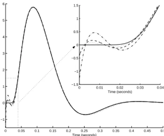
and γ. 0 0.05 0.1 0.15 0.2 0.25 0.3 0.35 0.4 0.45 0.5 −1 0 1 2 3 4 5 6 Time (seconds) 0 0.01 0.02 0.03 0.04 −1.5 −1 −0.5 0 0.5 1 1.5 Time (seconds)
Fig. 1. Impulse responses of the original system, of its 4th-order model for(α1; γ1) = (18.5; 37.0) (dashed line), for (α2; γ2) = (8.95; 47.9) (dot
line) and of its 4th-order Pad´e model (dashed-dot line)
Starting with the Laguerre spectrum of each function ˆfλ,µ(s)
computed for common values α and γ of the Laguerre parameters, the procedure of MIMO system reduction then follows:
1. Compute the Gram matricesΨλ,µand the vectors ~bλ,µrelative
to the transfer functions bfλ,µ(s).
2. Form the Gram matrix Ψ = Pλ,µΨλ,µ and the vector ~b =
P
λ,µ~bλ,µthen solveΨ~a = −~b for ~a = [a0a1... ar−1] T
.
3. Construct the reduced model bF (s) given in (20) by using (19)e for all the values of λ and µ.
Note that the numerators pλ,µ(s) could be optimized by solving
be
fλ,µ(ν∗i + γ − 2α) = ˆfλ,µ(νi∗+ γ − 2α)
for i= 1, 2, ..., r where νi∗stands for the negatives of the complex
conjugate of the zeros of q(s).
IV. NUMERICAL EXAMPLE
To illustrate the utility of the method we present a typical ap-plication of model reduction of an infinite-dimensional system. The system considered is a distributed RC circuit whose irrational transfer function is [15], [16] ˆ g(s) = 1 1 +sinh( √ RCs) √ RCs with RC= 1.
Fromgˆ(s), the first N = 150 coefficients of a Laguerre model are recursively computed using [17] for two different weight functions ̟1(t) = 1 and ̟2(t) = e−30t. The corresponding Laguerre
parameters (α1; γ1) = (18.5; 37.0) and (α2; γ2) = (8.95; 47.9)
used for the computation of the truncated Laguerre spectrum ofˆg(s) came from the optimization method described in [16], [18]. Using the technique presented in this paper the following 4th-order reduced models are derived as
beg1(s) = −0.397s 3+ 155.4s2 − 25589s + 1746201 s4+ 157.5s3+ 10611s2+ 239771s + 3493517, beg2(s) = −0.177s3+ 83.50s2− 15866s + 1209479 s4+ 113.8s3+ 7820s2+ 166458s + 2443337,
and are compared with the Pad´e approximation begP ad´e(s) =
−1.298s3+ 357.2s2− 46275s + 2693055
s4+ 205.6s3+ 15444s2+ 356292s + 5386110.
The impulse response of the original transfer function and those of the 4th-order models and Pad´e approximation are presented Fig. 1 and show the great accuracy of the presented model-reduction procedure. The time zoom near t = 0 underlines the role played
by the weight function ̟(t) = e−(γ−2α)t: a choice of γ > 2α,
as used to derive beg2(s), produces an improvement of the reduced
model quality around t = 0 (to a comparative detriment of the quality for t greater). If we define the relative weighted quadratic error by Q , hg − ˜g, g − ˜gi /hg, gi we obtain Q1 = 2.18 · 10−4
and Q2 = 6.10 · 10−4 for the Laguerre-Gram reduced models,
and QP ad´e = 1.32 · 10−3 (computed for the weighting function
̟(t) = 1) for the Pad´e model. These results confirm the great accuracy of the model reduction procedure.
V. CONCLUSION
An efficient procedure for model reduction of finite or infinite dimensional transfer function described by a Laguerre expansion has been presented. Based on a one-order operator in the Laplace domain is constructed a set of basis functions from which is applied a procedure of quadratic error minimization. The use of a weight function in the inner product definition permits a control of the time-error spreading of the reduced model. Integrals defining the required inner products are replaced by sums (finite in practice) expressed using the Laguerre spectrum of the original transfer function and can be computed recursively, allowing a numerically convenient calculation. We have shown that the reduced model preserves the first derivatives of the transfer function at a chosen point s= γ − α and has an impulse response that belongs to L2̟
¡
R+¢. The procedure has also been extended to MIMO systems. Presented work takes part inter alia of model reduction of infinite dimensional systems. An illustrative example has shown the efficiency of the procedure.
ACKNOWLEDGMENT
The authors wish to acknowledge the Brittany Region for financial support. They also would like to thank the reviewers for their valuable comments and suggestions.
REFERENCES
[1] P. R. Clement, “Laguerre functions in signal analysis and parameter identification,” Journal of the Franklin Institute, vol. 313, no. 2, pp. 85–95, 1982.
[2] B. Wahlberg, “System identification using Laguerre models,” IEEE
Trans. Automat. Contr., vol. 36, no. 5, pp. 551–562, 1991.
[3] C. T. Chou, M. Verhaegen, and R. Johansson, “Continuous-time identi-fication of SISO systems using Laguerre functions,” IEEE Trans. Signal
Processing, vol. 47, no. 2, pp. 349–362, 1999.
[4] P. M. M¨akil¨a, “Approximation of stable systems by Laguerre filters,”
Automatica, vol. 26, no. 2, pp. 333–345, 1990.
[5] ——, “Laguerre series approximation of infinite dimensional systems,”
Automatica, vol. 26, no. 6, pp. 985–995, 1990.
[6] G. A. Dumont, C. C. Zervos, and G. Pagean, “Laguerre-based adaptive control of pH in an industrial bleach plant extraction stage,” Automatica, vol. 26, no. 4, pp. 781–787, 1990.
[7] L. Knockaert and D. D. Zutter, “Laguerre-svd reduced-order modeling,”
IEEE Trans. Microwave Theory Tech., vol. 48, no. 9, pp. 1469–1475,
2000.
[8] ——, “Stable Laguerre-svd reduced-order modeling,” IEEE Trans.
Cir-cuits Syst. I, vol. 50, no. 4, pp. 576–579, 2003.
[9] Y. Chen, V. Balakrishnan, C. K. Koh, and K. Roy, “Model reduction in the time-domain using Laguerre polynomials and Krylov methods,” in
DATE’2002, Paris, France, Mar. 4–8, 2002, pp. 931–935.
[10] R. Malti, D. Maquin, and J. Ragot, “Some results on the convergence of transfer function expansion on Laguerre series,” in European Control
Conference, ECC’99, Karlsruhe, Germany, 31 Aug.–4 Sep. 1999.
[11] L. C. Calvez, Contribution `a l’´etude des propri´et´es de la transformation
Z et de la transformation de Laguerre. Applications `a l’analyse des signaux et circuits. Univ. de Brest, Brest, France: Th`ese de Doctorat d’Etat, 1973.
[12] F. Tricomi, “Transformazione di Laplace e polinami di Laguerre,” R. C.
Accad. Nat. dei Lincei, vol. 21, pp. 232–239, 1935.
[13] W. T. Weeks, “Numerical inversion of Laplace transforms using Laguerre functions,” J. ACM, vol. 13, pp. 419–426, 1966.
[14] H. Nagaoka, “Mullis-Roberts-type approximation for continuous-time linear systems,” Electronics and Communications in Japan, vol. 70, no. 10, p. part 1, 1987.
[15] S. P. Johnson and L. P. Huelsman, “A high-q distributed-lumped-active network configuration with zero real-part pole sensitivity,” Proc. IEEE, vol. 58, no. 3, pp. 491–492, 1970.
[16] R. Morvan, Mod´elisation de circuits et syst`emes de dimension infinie. Univ. de Brest, Brest, France: Th`ese de Doctorat, 2000.
[17] R. Morvan, N. Tanguy, P. Vilb´e, and L. C. Calvez, “Simplified algorithm for Laguerre approximation of URC networks,” Electronics Letters, vol. 35, no. 16, pp. 1299–1300, Aug. 1999.
[18] N. Tanguy, P. Vilb´e, and L. C. Calvez, “Optimum choice of free parameter in orthonormal approximations,” IEEE Trans. Automat. Contr., vol. 40, no. 10, pp. 1811–1813, Oct. 1995.