HAL Id: tel-01974511
https://tel.archives-ouvertes.fr/tel-01974511
Submitted on 8 Jan 2019HAL is a multi-disciplinary open access archive for the deposit and dissemination of sci-entific research documents, whether they are pub-lished or not. The documents may come from teaching and research institutions in France or abroad, or from public or private research centers.
L’archive ouverte pluridisciplinaire HAL, est destinée au dépôt et à la diffusion de documents scientifiques de niveau recherche, publiés ou non, émanant des établissements d’enseignement et de recherche français ou étrangers, des laboratoires publics ou privés.
Carlo Ieva
To cite this version:
Carlo Ieva. Unveiling source code latent knowledge : discovering program topoi. Programming Lan-guages [cs.PL]. Université Montpellier, 2018. English. �NNT : 2018MONTS024�. �tel-01974511�
En Informatique
École doctorale : Information, Structures, Systèmes Unité de recherche : LIRMM
Révéler le contenu latent du code source
A la découverte des topoi de programme
Unveiling Source Code Latent Knowledge
Discovering Program Topoi
Révéler le contenu latent du code source
A la découverte des topoi de programme
Unveiling Source Code Latent Knowledge
Discovering Program Topoi
Présentée par Carlo Ieva
Le 23 Novembre 2018
Sous la direction de Prof. Souhila Kaci
Devant le jury composé de
Michel Rueher, Professeur, Université Côte d’Azur, I3S, Nice Président du jury Yves Le Traon, Professeur, Université du Luxembourg, Luxembourg Rapporteur Lakhdar Sais, Professeur, Université d’Artois, CRIL, Lens Rapporteur Jérôme Azé, Professeur, Université de Montpellier, LIRMM, Montpellier Examinateur Roberto Di Cosmo, Professeur, Université Paris Diderot, INRIA Examinateur Samir Loudni, Maître de Conférences, Université de Caen-Normandie, GREYC, Caen Examinateur Clémentine Nebut, Maître de Conférences, Université de Montpellier, LIRMM, Montpellier Examinatrice Arnaud Gotlieb, Chief Research Scientist, Simula Research Lab., Lysaker, Norway Co-encadrant Nadjib Lazaar, Maître de Conférences, Université de Montpellier, LIRMM, Montpellier Co-encadrant
“You will become clever through your mistakes” reads a German proverb and doing a Ph.D. has surely to do with making mistakes. Whether I have become a clever person, I’ll let the reader be the judge, nonetheless, I learned a great deal. If I was asked to say what I learned in just one sentence then I would answer: a new way to look at things; this is for me what a Ph.D. really teaches you.
The path leading up to this point has not always been straightforward, learning is not a painless experience, and now is the moment to thank all those who helped me along the way. Thanks to my supervisors: Souhila Kaci, Arnaud Gotlieb and, Nadjib Lazaar, who patiently provided me an invaluable help. Thanks to Simula for creating the right conditions to make my Ph.D. possible. I would also like to express my very great appreciation to the reviewers Yves Le Traon and Lakhdar Sais who accepted to examine my thesis providing me their valuable feedback and thanks also to all jury members for being part of the committee.
During the development of long lifespan software systems, specification docu-ments can become outdated or can even disappear due to the turnover of soft-ware developers. Implementing new softsoft-ware releases or checking whether some user requirements are still valid thus becomes challenging. The only reliable de-velopment artifact in this context is source code but understanding source code of large projects is a time- and effort- consuming activity. This challenging problem can be addressed by extracting high-level (observable) capabilities of software systems. By automatically mining the source code and the available source-level documentation, it becomes possible to provide a significant help to the software developer in his/her program comprehension task.
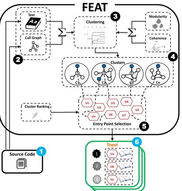
This thesis proposes a new method and a tool, called FEAT (FEature As Topoi), to address this problem. Our approach automatically extracts program topoi from source code analysis by using a three steps process: First, FEAT creates a model of a software system capturing both structural and semantic elements of the source code, augmented with code-level comments; Second, it creates groups of closely related functions through hierarchical agglomerative clustering; Third, within the context of every cluster, functions are ranked and selected, according to some structural properties, in order to form program topoi.
The contributions of the thesis is three-fold:
1. The notion of program topoi is introduced and discussed from a theoretical standpoint with respect to other notions used in program comprehension ; 2. At the core of the clustering method used in FEAT, we propose a new
hy-brid distance combining both semantic and structural elements automati-cally extracted from source code and comments. This distance is parametrized and the impact of the parameter is strongly assessed through a deep exper-imental evaluation ;
3. Our tool FEAT has been assessed in collaboration with Software Heritage (SH), a large-scale ambitious initiative whose aim is to collect, preserve and, share all publicly available source code on earth. We performed a large
experimental evaluation of FEAT on 600 open source projects of SH, coming from various domains and amounting to more than 25 MLOC (million lines of code).
Our results show that FEAT can handle projects of size up to 4,000 functions and several hundreds of files, which opens the door for its large-scale adoption for program comprehension.
Introduction
Le développement de projets open source à grande échelle implique de nom-breux développeurs distincts qui contribuent à la création de référentiels de code volumineux. À titre d’exemple, la version de juillet 2017 du noyau Linux (version 4.12), qui représente près de 20 lignes MLOC (lignes de code), a demandé l’effort de 329 développeurs, marquant une croissance de 1 MLOC par rapport à la ver-sion précédente. Ces chiffres montrent que, lorsqu’un nouveau développeur sou-haite devenir un contributeur, il fait face au problème de la compréhension d’une énorme quantité de code, organisée sous la forme d’un ensemble non classifié de fichiers et de fonctions.
Organiser le code de manière plus abstraite, plus proche de l’homme, est une tentative qui a suscité l’intérêt de la communauté du génie logiciel. Malheureu-sement, il n’existe pas de recette miracle ou bien d’outil connu pouvant apporter une aide concrète dans la gestion de grands bases de code.
Nous proposons une approche efficace à ce problème en extrayant automatique-ment des topoi de programmes, c’est à dire des listes ordonnées de noms de fonc-tions associés à un index de mots pertinents. Comment se passe le tri? Notre approche, nommée FEAT, ne considère pas toutes les fonctions comme égales: certaines d’entre elles sont considérées comme une passerelle vers la compréhen-sion de capacités de haut niveau observables d’un programme. Nous appelons ces fonctions spéciales points d’entrée et le critère de tri est basé sur la distance entre les fonctions du programme et les points d’entrée. Notre approche peut être résumé selon ses trois étapes principales:
1. Preprocessing. Le code source, avec ses commentaires, est analysé pour gé-nérer, pour chaque unité de code (un langage procédural ou une méthode orientée objet), un document textuel correspondant. En outre, une représen-tation graphique de la relation appelant-appelé (graphe d’appel) est égale-ment créée à cette étape.
2. Clustering. Les unités de code sont regroupées au moyen d’une classification par clustering hiérarchique par agglomération (HAC).
3. Sélection du point d’entrée. Dans le contexte de chaque cluster, les unités de code sont classées et celles placées à des positions plus élevées constitueront un topos de programme.
La contribution de cette thèse est triple:
1. FEAT est une nouvelle approche entièrement automatisée pour l’extraction de topoi de programme, basée sur le regroupement d’unités directement à partir du code source. Pour exploiter HAC, nous proposons une distance hybride originale combinant des éléments structurels et sémantiques du code source. HAC requiert la sélection d’une partition parmi toutes celles produites tout au long du processus de regroupement. Notre approche uti-lise un critère hybride basé sur la graph modularity [17] et la cohérence tex-tuelle [21] pour sélectionner automatiquement le paramètre approprié. 2. Des groupes d’unités de code doivent être analysés pour extraire le
pro-gramme topoi. Nous définissons un ensemble d’éléments structurels obte-nus à partir du code source et les utilisons pour créer une représentation alternative de clusters d’unités de code. L’analyse en composantes princi-pales, qui permet de traiter des données multidimensionnelles, nous per-met de mesurer la distance entre les unités de code et le point d’entrée idéal. Cette distance est la base du classement des unités de code présenté aux uti-lisateurs finaux.
3. Nous avons implémenté FEAT comme une plate-forme d’analyse logicielle polyvalente et réalisé une étude expérimentale sur une base ouverte de 600 projets logiciels. Au cours de l’évaluation, nous avons analysé FEAT sous plusieurs angles: l’étape de mise en grappe, l’efficacité de la découverte de topoi et l’évolutivité de l’approche.
Travaux connexes
Nos travaux s’inscrivent dans le domaine de la compréhension de programmes en se concentrant principalement sur l’extraction de fonctionnalités [68, 11, 45]. L’extraction de fonctionnalités vise à découvrir automatiquement les principales fonctionnalités d’un logiciel en analysant son code source ainsi que d’autres ar-tefacts. L’extraction de fonctionnalités est différente de la localisation de fonction-nalités, dont l’objectif est de localiser où et comment des fonctionnalités données sont implémentées [68]. La localisation nécessite que l’utilisateur fournisse une requête d’entrée dans laquelle la fonctionnalité recherchée est déjà connue,
tan-dis que l’extraction de la fonctionnalité tente de la découvrir automatiquement. Depuis plusieurs années, l’extraction de fonctionnalités de logiciels est considé-rée comme une activité dominante dans la compréghension de programmes. Ce-pendant, nous pouvons faire la distinction entre les approches de compréhension de programmes qui traitent la documentation des logiciels et celles qui traitent directement le code source.
Compréhension de programmes basée sur la documentation de logiciel
Dans [18], les techniques d’exploration de texte et de clustering sont utilisées pour extraire des descripteurs de fonctionnalités à partir des besoins de l’utili-sateur conservés dans des référentiels de logiciels. En combinant l’extraction de règles d’association et le k-plus proche-voisin, l’approche en question propose des recommandations sur d’autres descripteurs afin de renforcer un profil initial. McBurney et al. [48] ont récemment présenté quatre générateurs automatiques de liste de fonctionnalités des projets logiciels. Ils sélectionnent des phrases en anglais de la documentation du projet résumant les fonctionnalités.
Compréhension de programmes basée sur le Code source.[41] propose des
mo-dèles probabilistes basés sur l’analyse de code en utilisant Latent Dirichlet Alloca-tion pour découvrir des foncAlloca-tionnalités sous la forme de topics (foncAlloca-tions princi-pales dans le code). [50] présente un système de recommandation de code source pour la réutilisation de logiciels. Basé sur un modèle de fonctionnalité (une no-tion utilisée dans l’ingénierie de ligne de produit et la modélisano-tion de la variabi-lité logicielle), le système proposé tente de faire correspondre la description aux fonctionnalités pertinentes afin de recommander la réutilisation du code source existant à partir de référentiels de code source libre. [2] propose une analyse syn-taxique en langage naturel pour extraire automatiquement une ontologie du code source. Partant d’une ontologie légère ( it concept map), les auteurs développent une ontologie plus formelle basée sur des axiomes.
A l’inverse, FEAT est entièrement automatisé et ne nécessite aucune forme de d’entrainement de jeu de données ni aucune activité de modélisation supplémen-taire. FEAT utilise une technique d’apprentissage automatique non supervisée, ce qui simplifie grandement son utilisation et son application.
[37] utilise le clustering et le LSI (Latent Semantic Indexing) pour évaluer la si-milarité entre des parties du code source. Les termes les plus pertinents extraits de l’analyse LSI sont réutilisés pour l’étiquetage des clusters. FEAT exploite à la place l’exploration de texte et l’analyse de la structure de code pour guider la création de clusters.
Comparant à ces techniques, FEAT a deux éléments distinctifs. Premièrement, FEAT traite à la fois la documentation du logiciel et le code source en appli-quant simultanément des techniques d’analyse de code et de texte. Deuxième-ment, FEAT utilise HAC en supposant que les fonctions logicielles sont
organi-sées selon une certaine structure (cachée) pouvant être automatiquement décou-verte.
Contexte
Clustering appliqué au logiciel
Les méthodologies de clustering appliquées au logiciel créent un groupe d’en-tités, telles que des classes, des fonctions, etc. L’objectif de ces dernières est de faciliter la compréhension de la structure d’un système logiciel large et complexe [73].
Appliquer du clustering au logiciel nécessite l’identification des entités qui font l’objet du groupement. Plusieurs artefacts peuvent être choisis, mais le plus popu-laire est le code source [51]. La sélection des entités dépend fortement de l’objectif de l’approche à utiliser en clustering. Pour la restructuration de programmes à un niveau plus fin, les instructions d’appel de fonction sont choisies comme entités [84], tandis que pour des problèmes de conception, les entités [6] sont souvent des modules logiciels mais également des classes ou des routines.
L’extraction de faits à partir du code source peut s’effectuer selon deux approches conceptuelles différentes: structural et sémantique. Les approches basées sur la structure reposent sur des relations statiques entre entités: références de variable, appels de procédure, héritage, etc. Les approches sémantiques prennent en compte les informations tirées du domaine de connaissances lié au code source [36]. Les recherches sur l’application du clustering au logiciel adopte largement les ap-proches basées sur la structure, mais il convient de noter que le résultat produit par les approches sémantiques tend à être plus significatif. C’est pourquoi cer-tains essayent de combiner les deux méthodes [78].
La création de clusters est réalisée via un algorithme de classification. Le clus-tering est la forme la plus courante d’apprentissage non supervisé et la clé de ce type d’approches est la notion de distance entre les éléments à grouper et à séparer. Différentes mesures de distance donnent lieu à différents regroupements Il existe deux catégories d’algorithmes hiérarchiques: Ascendant (bottom-up) et descendant (top-down). Dans le clustering appliqué au logiciel et selon [33], les algorithmes descendants offrent un avantage par rapport aux algorithmes ascen-dants car les utilisateurs s’intéressent principalement à la structure révélée par les grands groupes créés au cours des premières étapes du processus. En revanche, les décisions erronées prises au cours des premières étapes peuvent affecter la manière dont les regroupements ascendants évoluent vers les grands
regroupe-Source Code
Clustering
C1 C2 C3 Cn
Cluster Ranking
Entry Point Selection U1 Clusters
FEAT
U2 U3 U4 U5 U6 U7 Un 4 Modularity 1 1 Topoi 2 3 Uc Ub Ua 6 Coherence Text Call Graph 2 3 5FIGURE1 –FEAT aperçu du processus
ments. La classification hiérarchique ascendante est toutefois la plus utilisée [82].
Notre approche nommée
FEAT
Au lieu d’utiliser uniquement du code source ou uniquement de la documenta-tion d’un système logiciel, FEAT combine les deux dans une même perspective grâce à une métrique de distance fusionnant la partie sémantique et les éléments structurels contenus dans le code source.
Certaines méthodes nécessitent une assistance humaine. Pour ne citer que quelques exemples: les méthodes basées sur les LDA nécessitent la saisie de paramètres statistiques difficiles à définir à l’avance. Les utilisateurs finaux doivent sélec-tionner une partition en clusters parmi d’autres. Les approches d’apprentissage supervisé nécessitant l’étiquetage de la formation Des exemples qui demandent beaucoup de temps et sont sujets aux problèmes de subjectivité. À la différence de ces approches, FEAT est entièrement automatisé, il applique des critères défi-nis formellement et sa sortie peut être directement utilisée pour l’extraction et/ou la localisation de fonctionnalités. Pour résumer les caractéristiques de FEAT:
• Les topoi de programme sont des structures concrètes résultantes d’une dé-finition formelle, utiles pour relever les défis de la compréhension automa-tisée de programmes.
ap-proches d’extraction et les apap-proches de la localisation des fonctionnalités. FEAT ne fait aucune distinction et permet de répondre aux deux tâches. • FEAT est basé sur un modèle de systèmes logiciels indépendant de tout
langage de programmation.
• FEAT ne nécessite aucune entrée supplémentaire autre que le code source. • FEAT est entièrement automatisé.
Un aperçu général de
FEAT
La compréhension d’un logiciel à travers son code source peut être abordée par deux approches conceptuelles: structurelle ou sémantique. Les approches basées sur la structure se concentrent sur les relations statiques entre les entités tandis que les approches sémantiques incluent tous les aspects de la connaissance du domaine d’un système qui peuvent être obtenus à partir des commentaires et des noms des identifiants [73]. L’extraction des principales fonctionnalités d’un logiciel peut tirer parti d’informations structurelles permettant d’identifier une fonctionnalité en tant qu’ensemble de unités de code contribuant à son implé-mentation. D’un point de vue sémantique, les parties d’un système présentant des points communs en termes de mots en langage naturel peuvent également être considérées comme faisant partie d’une même fonctionnalité d’un système. En d’autres termes, les approches structurelles et sémantiques véhiculent deux perspectives différentes et de valeurs inestimables. FEAT combine les deux pour obtenir une image plus précise des fonctionnalités proposées par un système lo-giciel. FEAT, dont les principaux éléments sont illustrés dans la Fig. 1, est basé sur un processus en trois étapes : pré-traitement (case notée 2 dans la Fig. 1), clus-tering (3 et 4 dans la Fig. 1) et sélection de points d’entrées (5 dans la Fig. 1). L’entrée de FEAT est un système logiciel représenté par du code source et des commentaires (1). À l’étape de prétraitement (2), FEAT analyse le code source et les commentaires, créant ainsi une représentation du système qui prend en charge la double hypothèse sous-jacente à l’approche.
Conclusion
FEAT automatise certaines pratiques courantes adoptées à la compréhension de programme (Sec. 2.2), telles que l’utilisation d’informations sémantiques et struc-turelles pour isoler les concepts sous la forme de clusters. Pour répondre au contexte de la compréhension du programme, nous avons adapté l’algorithme
de HAC en fournissant à la fois une nouvelle notion de distance (Sec. 4.5) et un critère d’arrêt (Sec. 4.7). L’application de PCA (Principal Component Analysis) à des unités de code a nécessité une étude approfondie des graphes d’appels du point de vue statistique (Sec. 4.8.1), révélant des modèles intéressants. Enfin, nous fournissons dans cette thèse une définition formelle de la notion nouvelle de topoi de programme (Def. 4.4). Nous montrons également que l’identification automatique de points d’entrée révélent certaines propriétés géométriques qui pourraient conduire d’intéressant développements. Enfin, la thèse présente une évaluation expérimentale approfondie incluant une expérience à grande échelle sur l’archive Software Heritage, soutenue par l’UNESCO.
1 Introduction 1
2 State of the Art 5
2.1 Introduction on Machine Learning . . . 5
2.1.1 Supervised Learning . . . 6
2.1.2 Unsupervised Learning . . . 12
2.2 Program Comprehension . . . 17
2.3 Program Comprehension via ML . . . 21
3 Background 25 3.1 Clustering . . . 25
3.1.1 Distances and HAC . . . 27
3.1.2 Merging criteria and HAC . . . 28
3.1.3 Software Clustering . . . 29
3.2 Principal Component Analysis . . . 30
3.3 Vector Space Model . . . 31
3.4 Latent Semantic Analysis . . . 32
3.5 Call Graph . . . 33
4 FEAT Approach 35 4.1 Genesis of FEAT . . . 35
4.2 A General Overview of FEAT . . . 36
4.3 Semantic Perspective over Code Units . . . 37
4.4 Structural Perspective over Code Units . . . 44
4.5 Hybrid Distance . . . 46
4.6 Distance over clusters . . . 46
4.7 Selecting a Partition in HAC . . . 48
4.7.1 Modularity . . . 49
4.7.2 Textual Coherence . . . 50
4.7.3 FEAT Cutting Criterion . . . 53
4.7.4 HAC Revised Algorithm . . . 53
4.8 Entry-Points Selection . . . 53
4.8.1 Ranking Units through PCA . . . 56
4.9 Program Topoi . . . 67
4.9.1 Entry-point Dictionary . . . 68
5 FEAT Tooling Support 71 5.1 Crystal Platform . . . 71
5.1.1 OSGi . . . 71
5.1.2 Business Process Modeling and Notation . . . 72
5.2 Crystal.FEAT . . . 73 5.2.1 Architecture . . . 73 5.2.2 FEAT Process . . . 74 5.2.3 User Interface . . . 76 6 Experimental Evaluation 81 6.1 Experimental Subjects . . . 81
6.2 Goodness of FEAT in Selecting Partitions . . . 82
6.3 Program Topoi Discovery Experiments . . . 84
6.3.1 Random Baseline Comparison . . . 86
6.3.2 No-clustering Experiment . . . 86
6.3.3 Impact of α, β Parameters . . . . 87
6.3.4 Applicability of Program Topoi . . . 91
6.4 Benefits of FEAT’s Hybrid Distance . . . 93
6.5 Scalability Evaluation . . . 95
6.5.1 FEAT at Software Heritage . . . 97
6.6 Threats to Validity . . . 99
2.1 High bias . . . 7
2.2 Good fit . . . 7
2.3 High variance . . . 7
2.4 Curse of dimensionality . . . 8
2.5 Kernel methods for support vector machines . . . 13
2.6 Separating hyperplane in SVM . . . 13
2.7 K-means and the shape of clusters . . . 15
3.1 HAC merging steps represented as a dendrogram . . . 27
4.1 Overview of FEAT . . . 38
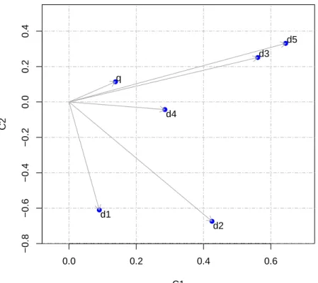
4.2 Unit-documents as geometric entities . . . 43
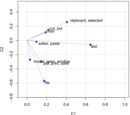
4.3 Plot of words in concept space . . . 45
4.4 Graph medoids example . . . 47
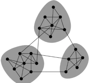
4.5 Division of a graph into clusters . . . 49
4.6 Graphics of several experiments on modularity . . . 51
4.7 Graphics of several experiments on textual coherence . . . 52
4.8 Plots of entry-point attributes of GEDIT. . . 60
4.9 Plots of entry-point attributes of MOSAIC . . . 61
4.10 Histograms of the norm of attributes’ vectors of two projects (GEDIT and MOSAIC, two clusters each). . . 63
4.11 Example of entry-point selection . . . 66
4.12 Plot of the entry-points selection’s example . . . 68
4.13 Plot of some entry-points extracted fromGEDIT . . . 69
5.1 CRYSTAL’s system architecture . . . 74
5.2 FEAT Process . . . 77
5.3 FEAT Web interface. List of projects . . . 78
5.4 FEAT Web interface. Program Topoi search . . . 79
5.5 FEAT Web interface. Program Topoi search, entry-point neighbor-hood . . . 79
6.1 FEAT’s performance experiment with changing α and β . . . . 89
6.2 FEAT’s performance with changing α and textual elements . . . . 90
6.4 “File print” entry-point neighborhood . . . 93 6.5 “Find text” entry-point neighborhood . . . 93 6.6 “Clipboard copy” entry-point neighborhood . . . 93 6.7 NCSA Mosaic web browser. Clustering of postscript printing feature. 95 6.8 NCSA Mosaic web browser. Clustering of browser window
cre-ation feature. . . 96 6.9 Correlation between running time and memory usage w.r.t. LOC,
number of units, size of the dictionary and, density of CG . . . 98 6.10 Experiment with Software Heritage . . . 100 6.11 Running time estimator . . . 102
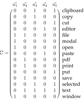
4.1 Distances between unit-documents’ vectors d1, . . . , d5 and query
vector qk . . . 43
4.2 KS test definition . . . 59 4.3 KS test results . . . 59 4.4 Ranking of units in the example of entry-point selection . . . 67 4.5 Ranking example of a program topos . . . 67 4.6 Example of Entry-points’ Dictionary . . . 70 5.1 CRYSTAL.FEAT commands’ list . . . 80 5.2 CRYSTAL.FEAT RESTful API . . . 80 6.1 Experimental results of the clustering step’s evaluation . . . 83 6.2 Random experiment . . . 87 6.3 No-HAC experiment . . . 87 6.4 Part of a program topos obtained from the analysis ofGEDIT . . . . 92 6.5 Feature location example inGEDIT . . . 92
6.6 Oracle used in the feature location experiment with MOSAIC . . . . 94 6.7 Comparison of FEAT with a LSI-based approach, while running
query: “font”. . . 95 6.8 Open Source software projects used in the scalability evaluation
experiment . . . 97 6.9 Summary of FEAT’s experiment at Software Heritage . . . 99
A Accuracy
AI Artificial Intelligence ANN Artificial Neural Network
BPMN Business Process Modeling and Notation CDF Cumulative Distribution Function
CG Call Graph
DNN Deep Neural Network
ECDF Empirical Cumulative Distribution Function FEAT FEature As Topoi
fn False Negatives fp False Positives
GDPR General Data Protection Regulation HAC Hierarchical Agglomerative Clustering IDC International Data Corporation
IR Information Retrieval K-S Kolmogorov-Smirnov
kNN k-Nearest Neighbor
LDA Latent Dirichlet Allocation LOC Lines of Code
LSA Latent Semantic Analysis LSI Latent Semantic Indexing ML Machine Learning
NB Naive Bayes
NLP Natural Language Processing OSGi Open Services Gateway initiative PCA Principal Component Analysis PC Program Comprehension
P Precision
RDBMS Relational Data Base Management System REST REpresentational State Transfer
RNN Recurrent Neural Network
R Recall
SOM Self Organizing Map
SVD Singular Value Decomposition SVM Support Vector Machines
tf-idf Term Frequency-Inverse Document Frequency tn True Negatives
tp True Positives VSM Vector Space Model
Introduction
Context and Challenges
Software-systems are developed to satisfy an identified set of user requirements. When the initial version of a system is developed, contractual documents are produced to agree on its capabilities. However, when the system evolves over a long period of time, the initial user requirements can become obsolete or even disappear. This mainly happens because of evolution of systems, maintenance, either corrective or adaptive, and personnel turn-over. When new business cases are considered, software engineers face the challenge of recovering the main ca-pabilities of a system from existing source code and low-level code documen-tation. Unfortunately, recovering user-observable capabilities is extremely hard since they are hidden behind the complexity of countless implementation details. Our work focuses on finding a cost-effective solution to this challenging problem by automatically extracting program topoi, which can be seen as summaries of the main capabilities of a program. Program topoi are given under the form of collec-tions of ordered code funccollec-tions along with a set of words (index) characterizing their purpose and a graph of their closer dependencies. Unlike requirements from external repositories or documents, which may be outdated, vague or incomplete, topoi extracted from source code are an actual and accurate representation of the capabilities of a system.
Several disciplines in the context of program understanding make use of a similar concept called feature. Wiegers in his book [81] provides the following definition: “. . . a feature is a set of logically related functional requirements that provides a
capabil-ity to the user and enables the satisfaction of a business objective”. This is a widely adopted definition in the literature but it is too abstract. Instead, program topoi are concrete objects targeted to source code, supported by a formal definition, and then suitable for automated computation. Nevertheless, extracting program topoi from source code is a complex task and to tackle this challenge we propose FEAT an approach and a tool for the automatic extraction of program topoi. FEAT acts in three steps:
1. Preprocessing. Creation of a model representing a software system. The model considers both structural and semantic elements of the system. 2. Clustering. By mining the available source code, possibly augmented with
code-level comments, hierarchical agglomerative clustering (HAC) groups similar code functions.
3. Entry-Point Selection. Functions within a cluster are then ranked and those fulfilling some structural requirements will be selected as program topos’ elements and stored.
Our work differs from those belonging to either feature extraction or location ar-eas (see a detailed overview in Sec.2.3) for the following rar-easons. First, FEAT extracts topoi which are structured summaries of the main capabilities of the pro-gram, while features are usually just informal description of software character-istics. Second, in FEAT the difference between feature extraction and feature location is not so urgent; one can employ topoi to discover system capabilities but also for looking for those he/she already knows.
Contribution of the Thesis
FEAT is a novel, fully automated approach for program topoi creation based on clustering and ranking code functions directly from source code. Along the path which led us to the current definition of the approach, we devised some original contributions which are listed as follows:
1. For an effective application of HAC to software systems, we propose an original hybrid distance combining structural and semantic elements of source code (Sec. 4.5). HAC requires the selection of a partition among all those produced along the clustering process. FEAT makes use of a hybrid crite-rion based on graph modularity [17] and textual coherence [21] to automatically select the appropriate partition (Sec. 4.7).
2. Clusters of code functions need to be further analyzed to extract program topoi. We define the concept of entry-point to accomplish this. Entry-points
are an alternative way to look at functions, they are based on a set of struc-tural properties coming from call graphs. Entry-points allow us: (i) to cre-ate a space in which functions can be trecre-ated as geometric objects, and (ii) to evaluate how representative they are in terms of a system’s capabilities. We employ PCA (Principal Component Analysis) for entry-point selection (Sec. 4.8). We published this results in a conference paper presented at IAAI 30th Innovative Application of Artificial Intelligence [30] and in a paper published in IEEE Transactions on Reliability journal [31].
3. We implemented FEAT on top of a general-purpose software analysis plat-form and perplat-formed an experimental study over many open-source soft-ware projects. Softsoft-ware Heritage1(SH) is an initiative owned by Inria whose
aim is to collect, preserve and, share all publicly available source code. We processed 600 projects coming from various domains amounting to more than 25 MLOC (lines of code). During the evaluation we analyzed FEAT under several perspectives: the clustering step, effectiveness in topoi dis-covery and search, and scalability of the approach.
Organization of the Thesis
The thesis is organized as follows. Chap. 2 presents the current state of the art in the various disciplines touched by this thesis. Chap. 3 gives the necessary back-ground on clustering, distance notions, PCA, call graphs, etc. Chap. 4 details the three main steps of FEAT with all the aspects we needed to handle in order to ap-ply techniques such as HAC, PCA, etc. to source code analysis. Chap. 5 describes CRYSTAL the platform we designed to host FEAT. Chap. 6 gives the experimen-tal results obtained with FEAT on several open-source software projects. Finally, Chap. 7 draws conclusions and presents some perspectives to this work.
State of the Art
The chapter provides an overview of the state of the art of the main topics at the basis of this work: machine learning, program comprehension and, the research done so far in the domain located at their intersection.
2.1
Introduction on Machine Learning
Answering the question “what is machine learning (ML)?” can be tricky because ML is a really vast subject. In 1959 Arthur Samuel, a pioneer in the field of artifi-cial intelligence (AI), coined the term machine learning [70]. He focused on cogni-tive computing1and, while he was working on a program capable of learning how
to play chess, he gave the following definition: “Machine Learning: Field of study that gives computers the ability to learn without being explicitly programmed.”. Tom Mitchell, another renowned researcher in ML, provided a more precise definition of machine learning in 1998: “A computer program is said to learn from experience E with respect to some task T and some performance measure P , if its performance on T , as measured by P , improves with experience E.”
Hence, although machine learning is a field within computer science, it differs from traditional computational approaches. In traditional computing, algorithms are sets of explicitly programmed instructions used by computers to calculate or solve problems while in ML algorithms allow for computers to train on data inputs and build models to accomplish tasks.
1. Discipline that studies hardware platform and/or software systems that mimic the way the human brain works.
Both Samuel’s and Mitchell’s definitions clearly explain the goal for ML. The way we reach this goal is through ML algorithms. Let us see the main categories into which they are divided. The first category is (i) supervised learning, which trains algorithms based on example input and output data that is labeled by humans, and the second is (ii) unsupervised learning which provides the algorithm with no labeled data in order to allow it to find a structure within its input data.
2.1.1
Supervised Learning
Supervised learning algorithms can be further divided according to the output domain. If the output consists in one or more continuous variables we apply regression predictive modeling that is the task of approximating a mapping func-tion (f ) from input variables (X) to a continuous output variable (Y ). On the other hand, a supervised learning problem where the answer to be learned is one of finitely many possible values is called classification.
Bias-variance Tradeoff
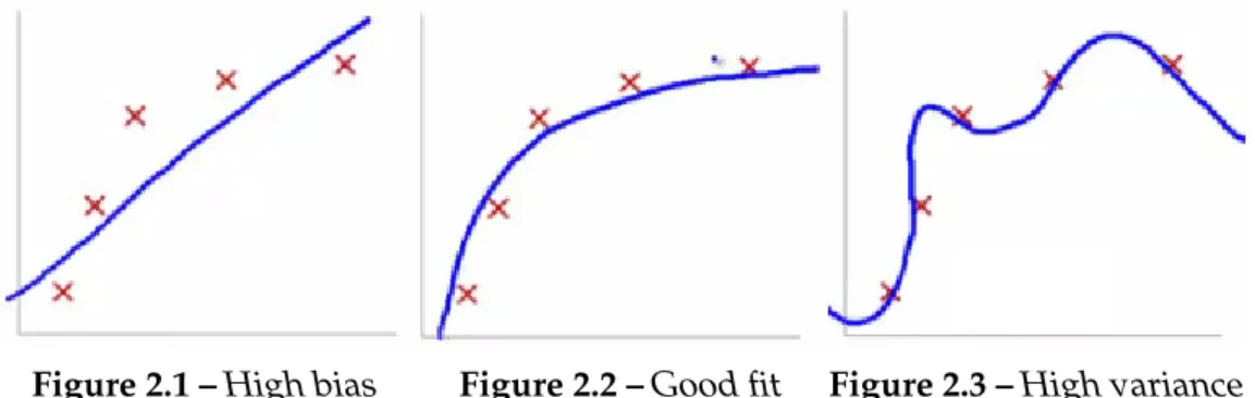
There are challenging aspects related to supervised learning algorithms. Behind any model there are some assumptions, but if they are too simplistic then the model generalizes well but does not fit the data (underfitting). This makes the model biased (see Fig. 2.1). On the other hand if the model fits the training data really well this is obtained at the expense of generalization which is called over-fitting (see Fig. 2.3). Overover-fitting occurs when a model corresponds too closely to the training set but fails when classifies new, unseen data. The problem of satis-fying both these two needs at the same time goes under the name of bias-variance tradeoff [44].
The Curse of Dimensionality
Modeling a classifier requires the selection of features. Features, also called vari-ables or attributes, are the basic elements of the training data and their selection is needed for building the model representing a classifier. We can think of features as descriptors for each object in our domain. If we selected too few features then our classifier would perform poorly (i.e. classify animal species just by single ani-mals’ color). An obvious solution to this problem is to add more features in order to make our model more complex and flexible. But, we cannot add to the model as many features as we wish while the training set remains the same. If they are too many, we have to face the curse of dimensionality [7].
Figure 2.1 –High bias Figure 2.2 –Good fit Figure 2.3 –High variance
One side effect of the curse of dimensionality is overfitting. This happens because adding dimensions to our model will make the feature space grow exponentially and consequently it becomes sparser and sparser. Because of this sparsity, it is easier to find a hyperplane perfectly separating the training examples; our clas-sifier is perfectly learning all the peculiarities of the training dataset even its ex-ceptions but it will fail on real-world data because of overfitting.
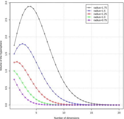
Another side effect of the curse of dimensionality is that sparsity is not uniformly distributed. This is a bit surprising, let us try to explain it through an example. Imagine a unit square that represents a 2D feature space. The average of the feature space is the center of this square, and all points within unit distance are inside a unit circle inscribed into the square. In 2D the center of the search space is ≈ 78% of the total. But, as we increase the number of dimensions, the center becomes smaller and smaller; in 3D it is ≈ 52% and in 8D it is ≈ 2%. Fig. 2.4 shows a graph of the volume of 5 hyperspheres, with increasing value of radius, and its relationship with the number of dimensions. The graph clearly shows how fast the volume goes to zero as the number of dimensions increases. Though it is hard to be visualized, we can say that nearly all of the high-dimensional space is “far away” from the centre or, in other words, the high-dimensional unit hypercube can be said to consist almost entirely of the “corners” of the hypercube, with almost no “middle”. In this scenario, where all the points are so distant from the center, distance metrics like the Euclidean distance are useless because there is not a significant difference between the maximum and minimum distance [3]. If we had an infinite number of training samples then we could use an infinite number of features to train the perfect classifier and then avoid the curse of di-mensionality. In reality a rule of thumb is: the smaller the size of the training dataset, the fewer the features that should be used. It is important to highlight that the feature space grows exponentially with the number of dimensions [7] and so the num-ber of examples should do accordingly. Feature selection can be a hard task to be accomplished. To tackle this challenge, techniques like Principal Component Analysis (PCA), which finds a linear subspace of the feature space with lower dimensionality (more on PCA in Chap. 3), can be used.
● ● ● ● ● ● ● ● ● ● ● ● ● ● ● ● ● ● ● ● ● ● ● ● ● ● ● ● ● ●● ● ●● ● ● ●● ● 5 10 15 20 0.0 0.5 1.0 1.5 2.0 2.5 3.0 Number of dimensions V olume of the h ypersphere ● radius=1.75 radius=1.5 radius=1.25 radius=1.0 radius=0.75
Figure 2.4 –Volume of the hypersphere decreases when the dimensionality increases.
Cross-validation
Overfitting is clearly a main concern for several supervised learning techniques. Another approach commonly adopted to overcome overfitting is cross-validation [52]. Basically, it splits the training dataset in two and the classifier is trained on just one subset of the examples. When the training is completed the remaining part is used for testing and evaluate the performance of the classifier. This approach called holdout is the basis for more advanced models like: K-fold and, leave-one-out. After this overview about supervised learning and its challenging aspects, let us now see some practical examples of supervised learning methods through a selection of the most representative ones.
Decision Trees
A most widely used method for approximating discrete-valued functions is de-cision tree learning. Learned trees represent an approximation of an unknown target function f : X 7→ Y . They belong to the family of inductive inference algo-rithms (i.e. inferring the general from the specific). Training examples are pairs
hXi, Yii where every Xi is a feature vector and Yia discrete value. By walking the
tree from the root to the leaves, decision trees classify instances. At each node the algorithm tests one attribute of the instance and selects the next branch to take on the basis of the possible values for this attribute. This step is repeated until the algorithm reaches a leaf indicating a Y value [52].
The basic algorithm for learning decision trees is ID3 [62], successively super-seded by C4.5 [63]. ID3 builds a tree top-down by answering the question “which is the best attribute to be tested ?”. The best attribute, that is the best one in sep-arating the training examples according to their target classification, is selected on the basis of a statistical measure called information gain. Then, the algorithm moves down the tree and repeats the same question for each branch. This process goes on until all data is classified perfectly or it runs out of attributes.
There are some issues related to the basic ID3 algorithm, first of all overfitting which occurs with noisy data leading to the construction of more complex trees perfectly fitting the wrong data. Random forest [29] is an algorithm derived from decision trees and it is designed to address ID3 overfitting problem. Instead of applying the ID3 algorithm on the whole dataset, dataset is separated into sub-sets leading to the construction of several decision trees, decisions are made by a voting mechanism. C4.5 algorithm, though sharing the basic mechanism of ID3, brought some improvements to its ancestor like the capacity of dealing with missing attributes values or attributes with continuous values.
Artificial Neural Networks
The development of artificial neural networks (ANNs) has been inspired by the study of learning mechanisms in biological neural systems. These systems are made of a web of interconnected units (neurons) interacting through connections (axons and synapses) with other units.
The general structure of a ANN can be thought as made of three layers: input layer, hidden layer and output layer. The input layer is connected to the source which can be sensor data, symbolic data, feature vectors, etc. The units in the hidden layer connect inputs with outputs and it is where the actual learning happens. Each of these units computes a single real-valued value based on a weighted combination of its inputs. Units’ interconnections in ANNs can form several type of graphs: directed or undirected, cyclic or acyclic. If the connec-tions in a neural network do not form any cycle they are called feedforward neural network. In these networks the information flows from the input to the output layer through the hidden layer(s). No cycle or loops are present which distin-guish them from recurrent neural networks (RNN).
linear unit and, sigmoid. Perceptron [49], which itself is a binary classifier, takes a vector of real-valued inputs and calculates a linear combination of these inputs. The output can be 1 or −1. Each input has an associated weight and learning a perceptron is about choosing values for the weights. A perceptron can represent only examples that can be linearly separated by a hyperplane in a n-dimensional space (n input points).
To overcome the limit about linearly separable samples it is not enough to add more layers; multiple layers of cascaded linear units still produce only linear functions. We need a unit whose output is a non-linear function of its inputs. One solution is the sigmoid unit (the name comes from the characteristic S-shaped curve) whose output ranges between 0 and 1, increasing monotonically with its input [52]. Sigmoid unit, like the perceptron, first computes a linear combination of its inputs and then applies a threshold to the result but, differently from per-ceptron, in sigmoid’s case the output is a continuous function of its input. The al-gorithm to learn the weights in a multilayer network is backpropagation [8], based on gradient descent optimization algorithm. It attempts to minimize the squared error between the network output values and the target values for these outputs. When there are multiple hidden layers between the input and the output layers then we call the ANN a deep neural network (DNN).
One final remark about ANNs. The European Union recently introduced the Gen-eral Data Protection Regulation (GDPR) that states the so-called right to explana-tion. Some of the articles of GDPR can be interpreted as requiring explanation of the decision made by a machine learning algorithm when it is applied to a human subject. This can clearly affect the adoption of ANNs in certain domains; provide an interpretation of the decisions made by neural networks it is very hard and practically impossible in DNNs.
Naive Bayes Classifier
Bayesian learning belong to a family of techniques based on statistical infer-ence. The assumptions lying at their basis is that the input data of the classifica-tion problem follow some probability distribuclassifica-tion. Bayesian learning estimates a mapping function between input and output data by means of the Bayes theorem. Its application can be challenging when dealing with many variables because of the difficulty of both computing and having samples of all joint probability com-binations. A solution to this problem comes from an approach, which is widely used in the field of text classification, called naive Bayes (NB). It is called naive because it assumes that all input variables are conditionally independent2 [26]
2. Two random variables X and Y are conditionally independent given a third random vari-able Z if and only if, given any value of Z, the probability distribution of X is the same for all values of Y and the probability distribution of Y is the same for all values of X.
hence dramatically simplifying the classification function (the number of needed parameters is reduced from exponential to linear in the number of variables). NB belongs to a category called generative classifiers which is in contrast with those called discriminative classifiers. A generative classifier learns the model be-hind the training data making assumptions about its distribution. On this basis, it can even generate unseen data. Instead, discriminative classifiers make fewer assumptions on the data and just learn boundary between classes. The choice between the two categories is determined by the training set size. With a rich training set, discriminative classifiers outperforms generative ones [60]. But, in case of few data a generative model, with the addition of some domain knowl-edge, can become the first choice.
In NB the training set is made of objects (which are feature vectors) and classes to which the objects belong. The algorithm requires the prior probability of an object occurring in a class P (C) and P (xk|C) that is the conditional probability
of attribute xk occurring in an object of class C. These probabilities are usually
unknown and then estimated from the training set. This way NB indicates which class C best represents a given object x by the conditional probability P (C|x) [44]. Despite its simplicity, NB, in some domains, showed performance similar to ANNs or decision trees.
K-nearest Neighbor
When it comes about making decisions on a ML approach it is really important to have a sufficient understanding on the problem at hand. Is it a nonlinear problem and its class boundaries cannot be approximated well with linear hyperplanes? Then a nonlinear classifier will be more accurate than a linear one. If the problem is linear, then it is best to use a simpler linear classifier. So far we have seen a nonlinear classifier (decision trees), a linear classifier (NB) and a mixed one depending on its structure (ANNs). The next two are nonlinear classifiers. Let us start with the simplest one.
k-nearest neighbor (kNN) [5] is one of the simplest classification algorithms. It is a non parametric classifier, meaning that it does not rely on any assumption about the distribution of the underlying data. Put simply, it builds a model for classification just from the data itself. This makes kNN a good candidate for a preliminary classification study when there is little a priori knowledge about the data distribution.
kNN is also defined a lazy algorithm because it does not have any training phase; it does not try to infer any generalization from the data.
kNN’s output is a class membership assigned to a test element by the majority class of its k closest neighbors. We can have 1NN, but it is too sensitive to outliers or misclassified elements, usually a value k > 1 is chosen [44].
Support Vector Machines
Support vector machines (SVM) [79] are binary, discriminative classifiers. They learn an optimal hyperplane separating the training examples in two classes. SVMs are known to be capable of classifying data which are not linearly sepa-rable and they accomplish this through their key element: kernel functions [72]. Kernel functions take the input space and transform it into a higher dimensional one. This transformation allows linear classifier to separate non linear problems. The key aspects of the approach based on SVMs with kernel functions are:
• Data items are embedded into a vector space called the feature space. • Linear relations are sought among the images of the data items in the feature
space.
• The algorithm for the computation of a separating hyperplane does not need the coordinates of the embedded points, only the pairwise inner prod-ucts.
• The pairwise inner products can be computed efficiently directly from the original data items using a kernel function.
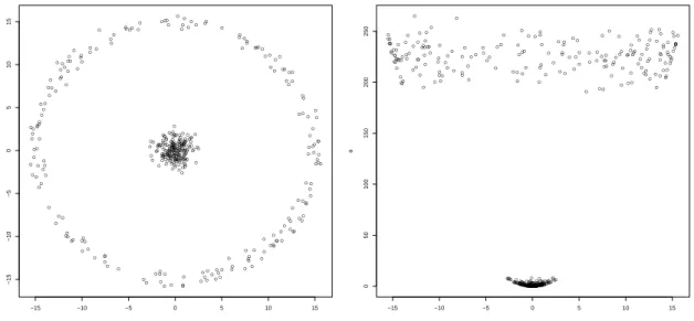
These aspects are illustrated in Fig. 2.5. The left side of the figure shows a non-linear pattern but by applying a kernel like φ(x, y) = x2 + y2 the data becomes
linearly separable as it is shown on the right side plot. In the feature space, where data can be linearly separated, SVM, of all possible decision boundaries that could be chosen to separate the dataset for classification, chooses the deci-sion boundary (separating hyperplane) which is the most distant from the points (support vectors) nearest to the said decision boundary from both classes (see Fig. 2.6).
In conclusion, SVM is a very effective tool; it uses only a small subset of training points (support vectors) to classify data, it is versatile: different kernel functions can be specified to fit domain specific problems.
2.1.2
Unsupervised Learning
In unsupervised learning, the training data consists of a set of input vectors with-out any corresponding target values. The goal in such problems may be to
dis-● ● ● ● ● ● ●● ● ● ● ● ● ● ● ● ● ● ●● ● ● ● ● ● ●● ● ● ●● ● ● ● ● ● ● ● ● ● ● ● ● ● ● ● ● ● ● ● ● ● ● ● ● ● ● ● ● ● ● ● ●● ● ● ● ● ● ● ● ●● ● ● ●● ● ● ● ● ● ● ● ● ●●● ● ●● ● ● ● ● ● ● ● ● ● ● ● ● ● ● ● ● ● ● ● ● ● ● ● ● ● ● ● ● ● ● ● ● ● ● ● ● ● ● ● ● ● ● ● ● ● ● ● ● ● ● ● ● ● ● ● ● ● ● ● ● ● ● ● ● ● ● ● ● ● ● ● ● ● ●● ● ● ● ● ● ● ● ● ● ● ● ● ● ● ● ● ● ● ●● ● ● ● ● ● ● ● ● ● ● ● ● ● ● ● ● ● ● ● ● ● ● ● ● ● ● ● ● ● ● ● ● ● ● ● ● ● ● ● ● ● ● ● ● ● ● ● ● ● ● ● ● ● ● ● ● ● ● ● ● ● ● ● ● ● ● ● ● ● ● ● ● ● ● ● ● ● ● ● ● ● ● ● ● ● ● ● ● ● ● ● ● ● ● ● ● ● ● ● ● ● ● ● ● ● ● ● ● ● ● ● ● ● ● ● ● ● ● ● ● ● ● ● ● ● ● ● ● ● ● ● ● ● ● ● ● ● ● ● ● ● ● ● ● ● ● ● ● ● ● ● ● ● ● ● ● ● ● ● ● ● ● ● ● ● ● ● ● ● ● ● ● ● ● ● ● ● ● ● ● ● ● ● ● ● ● ● ● ● ● ● ● ● ● ● ● ● ● ● ● ● ● ● ● ● ● ● ● ● ● ● ● ● ● −15 −10 −5 0 5 10 15 −15 −10 −5 0 5 10 15 x y ● ● ● ● ● ● ●● ● ● ● ● ● ● ● ● ●●● ● ●●●● ● ●● ● ● ●●● ● ● ●● ● ● ● ● ● ● ● ● ● ●●●● ● ●● ● ● ● ●●● ● ● ●● ●●●● ●●● ●●●● ● ● ●● ● ● ● ● ● ●●● ●●●●●●●●●●●●●●●● ● ● ● ● ● ●●●●● ● ● ●● ●●● ●● ● ● ● ● ● ●●●● ● ● ●● ● ● ● ● ● ● ● ● ● ● ● ●● ● ●●●●●● ●●●● ●●● ●●●● ●● ●●●● ● ● ●●●●●● ● ● ● ●● ● ●●●● ● ● ● ● ● ● ● ●● ● ●● ● ● ● ● ● ● ● ● ● ● ● ● ● ● ● ● ● ● ● ● ● ● ● ● ● ● ● ● ● ● ● ● ● ● ● ● ● ● ● ● ● ● ● ● ● ● ● ● ● ● ● ● ● ● ● ● ● ● ● ● ● ● ● ● ● ● ● ● ● ● ● ● ● ● ● ● ● ● ● ● ● ● ● ● ● ● ● ● ● ● ● ● ● ● ● ● ● ● ● ● ● ● ● ● ● ● ● ● ●● ● ● ● ● ● ● ● ● ● ● ● ● ● ● ● ● ● ● ● ● ● ● ● ● ● ● ● ●● ● ● ● ● ● ● ● ● ● ● ● ● ● ● ● ● ● ● ● ● ● ● ● ● ● ● ● ● ● ● ● ● ● ● ● ● ● ● ● ● ● ● ● ● ● ● ● ● ● ● ● ● ● ● ● ● ● ● ● ● ● −15 −10 −5 0 5 10 15 0 50 100 150 200 250 x φ
Figure 2.5 – The function φ = x2 + y2 embeds the data into a feature space where the
nonlinear pattern now becomes linearly separable.
cover underlying structures of a dataset like groups or create summaries of it. Two representative tasks, achievable through unsupervised learning algorithms, are clustering data into groups by similarity and dimensionality reduction which compresses the data while revealing its latent structure.
It is not always easy to understand the output of unsupervised learning algo-rithms; they can figure out on their own how to sort different classes of elements, but they might also add unforeseen and undesired categories to deal with creat-ing clutter instead of order.
Since there are no labeled examples, a challenging aspect of such approaches is
Figure 2.6 – SVM’s separating hyperplane maximizing margin among support vectors belonging to the two classes.
evaluating their performance; what is usually done is to create either ad-hoc met-rics or exploiting some domain-specific knowledge.
Let us see an overview of some of the most widely adopted algorithms in unsu-pervised learning.
K-means
Clustering is the most common form of unsupervised learning. It organizes data instances into similarity groups, called clusters such that the data instances in the same cluster are similar to each other and data instances in different clusters are very different from each other [42, 44]. One might wonder whether there is such a big difference between classification and clustering; after all, in both cases we have a partition of data items into groups. But the difference between the two problems lies at their foundation. In classification we want to replicate the criterion a human used to distinguish elements of the data. In clustering there is no such guidance and the key input is the distance measure.
Clustering algorithms are divided into two broad categories: flat clustering and hierarchical clustering. The former algorithms do not create any structure among clusters whereas the latter provide an informative hierarchy [44].
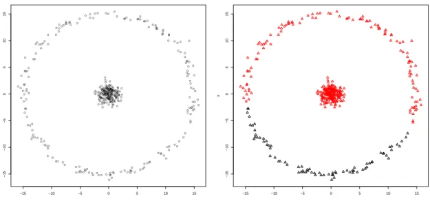
K-means [27] is the most important flat clustering algorithm. The goal of this al-gorithm is to find K groups in the data. The alal-gorithm works iteratively to assign each data point to one of K groups based on the features that are provided. Data points are clustered based on feature similarity. K-means aims at minimizing the average squared Euclidean distance of data points from their cluster centers. A cluster center is represented by the mean or centroid of the elements in a cluster. The K in K-means indicates the number of clusters and it is an input parameter. The algorithm (1) randomly chooses K data points (seeds) as centroids and (2) iteratively reassigns data points to clusters and update centroids until a termina-tion conditermina-tion is met. Some drawbacks of this simple and effective algorithm are: (1) a prespecified number of clusters that can be hard to be provided, (2) sensi-tivity to outliers, (3) the selection of initial seeds affects the search which can get stuck in a local minimum and, (4) the assumption about the shape of the clusters; K-means works best with non-overlapping spherical clusters (see Fig. 2.7).
Hierarchical Clustering
Hierarchical clustering establishes a hierarchy among clusters which can be cated either with top-down or bottom-up algorithms. Top-down clustering
re-●● ● ● ● ● ● ●● ● ● ● ● ● ● ● ● ● ● ● ● ● ● ● ● ● ● ● ● ● ● ● ● ● ● ● ● ● ● ● ● ● ● ● ● ● ● ● ● ● ● ● ● ● ● ● ● ●● ● ● ● ● ● ● ● ● ● ● ● ● ● ● ● ● ● ● ● ● ● ● ● ● ● ● ● ● ● ● ● ● ● ● ● ● ● ● ● ● ● ● ● ● ● ● ● ● ● ● ● ● ● ● ● ● ● ● ●● ● ● ● ● ● ● ● ● ● ● ● ● ● ● ● ● ● ● ● ● ● ● ●● ● ●● ● ● ● ● ● ●● ● ● ● ● ● ● ●● ● ● ● ● ● ● ● ● ● ● ● ● ● ● ● ● ● ● ● ● ●● ● ● ● ● ● ● ● ● ● ● ● ● ● ● ● ● ● ● ● ● ● ● ● ● ● ● ● ● ● ● ● ● ● ● ● ● ● ● ● ● ● ● ● ● ● ● ● ● ● ● ● ● ● ● ● ● ● ● ● ● ● ● ● ● ● ● ● ● ● ● ● ● ● ● ● ● ● ● ● ● ● ● ● ● ● ● ● ● ● ● ● ● ● ● ● ● ● ● ● ● ● ● ● ● ● ● ● ● ● ● ● ● ● ● ● ● ● ● ● ● ● ● ● ● ● ● ● ● ● ● ● ● ● ● ● ● ● ● ● ● ● ● ● ● ● ● ● ● ● ● ● ● ● ● ● ● ● ● ● ● ● ● ● ● ● ● ● ● ● ● ● ● ● ● ● ● ● ● ● ● ● ● ● ● ● ● ● ● ● ● ● ● ● ● ● ● ● ● ● ● ● ● ● ● ● ● ● ● ● ● ● ● ● ● ● ● ● −15 −10 −5 0 5 10 15 −15 −10 −5 0 5 10 15 x y −15 −10 −5 0 5 10 15 −15 −10 −5 0 5 10 15 x y
Figure 2.7 –It is easy for a human to see the two clusters in the left plot. The right one shows the clustering (red and black triangles) created by K-means. The algorithm fails in finding the two clusters in this dataset because it tries to find two centers with non-overlapping spheres around them.
quires a criterion to split clusters. It proceeds by splitting clusters recursively until individual data points are reached. Bottom-up algorithms, also called Hier-archical Agglomerative Clustering (HAC), start by considering each data point as a singleton cluster and then incrementally merge pairs of clusters until either the process is stopped or all clusters are merged into a single final cluster [44].
Unlike the K-means algorithm, which uses only the centroids in distance compu-tation, hierarchical clustering may use anyone of several methods to determine the distance between two clusters.
Hierarchical clustering has several advantages over K-means. It can take any distance measure, can handle clusters of any shape, the resulting structure can be really informative. Hierarchical clustering on the other hand are computation-ally demanding both in terms of space and time. Also some criteria used to merge clusters suffer from the presence of outliers. More details about hierarchical clus-tering will be given in Chap. 3.
One-class SVM
In the supervised learning section we have seen SVMs. They train a classifier on a training set so that examples belong to one of two classes. This is clearly a su-pervised learning model but actually SVM can be used also in contexts where we can have a large majority of positive examples and we want to find the negative
ones. This peculiar application of SVMs is called one-class SVM [71].
In one-class SVM, the support vector model is trained on data that has only one class, which is the normal class. It infers the properties of normal cases and from these properties can predict which examples are unlike the normal examples. This is useful for anomaly detection because the scarcity of training examples is what defines anomalies: that is, typically there are very few examples of the network intrusion, fraud, or other anomalous behavior. Then when new data are encountered their position relative to the normal data (or inliers) from training can be used to determine whether it is out of class or not; in other words, whether it is unusual or not.
One-class SVM have been applied to several different contexts like: anomaly de-tection, novelty dede-tection, fraud dede-tection, outlier dede-tection, etc. proving that is a very versatile and useful approach to unsupervised learning.
Autoencoder
An autoencoder is a neural network that has three layers: an input layer (x), a hidden (encoding) layer (h), and a decoding layer (y). The network is trained to reconstruct its inputs by minimizing the difference between input and output, which forces the hidden layer to try to learn good representations of the inputs. Autoencoders are designed to be unable to perfectly reproduce the input. They are forced to learn an approximation, a representation that resembles the input data. Being forced to set higher priority to some aspects of the input usually leads autoencoders to learn useful properties of the data [28].
One way to obtain useful features from the autoencoder is to constrain h (hidden layer) to have a smaller dimension than x (input layer). An autoencoder whose code dimension is less than the input dimension is called undercomplete. Learn-ing an undercomplete representation forces the autoencoder to capture the most salient features of the training data.
Learning autoencoders proved to be difficult because the several encodings of the input code compete to set the same small amount of dimensions. This has been solved through sparse autoencoders [66]. In a sparse autoencoder, there are actually more hidden units than inputs, but only a small number of the hidden units are allowed to be active at the same time.
Traditionally, autoencoders have been used for dimensionality reduction, feature learning and, noise removal. Autoencoders are quite similar to PCA (principal component analysis) (see Chap. 3 for a more detailed discussion on PCA) in terms of potential applications. One advantage of autoencoders over PCA is the capac-ity of learning nonlinear transformations.
Self Organizing Map
Self organizing map (SOM) are a ANN-based technique for dimensionality reduc-tion. More specifically they are used for creating visual representation of high dimensional data in 2D. Sometimes they are also called Kohonen maps or net-works [35] according to the name of the Finnish professor who introduced them in the 1980s. Teuvo Kohonen writes “The SOM is a new, effective software tool for the visualization of high-dimensional data. It converts complex, nonlinear statistical re-lationships between high-dimensional data items into simple geometric rere-lationships on a low-dimensional display. As it thereby compresses information while preserving the most important topological and metric relationships of the primary data items on the display, it may also be thought to produce some kind of abstractions.”
The visible part of a SOM is the map space, which is either a rectangular or hexag-onal grid of nodes (neurons). Each node has an associated weight vector with the same dimensionality of the input data and it represents node’s position in the input space. After an initialization step, where weight vectors are initialized at random, SOM algorithm picks an input vector and select the best matching unit (BMU) that is the closest node to the input vector. Then, BMU and its neighbor-hood is moved towards the input vector. The algorithm iterates until it meets a stabilization criterion.
SOM are said to preserve the topological structure of the input data set which simply means that if two input vectors are close together, then the neurons related to those input vectors will also be close together. SOM can also act as classifier for new data by looking for the node with the closest weight vector to the data vector.
Finally, SOM can be considered as a nonlinear generalization of principal compo-nent analysis (PCA).
2.2
Program Comprehension
Program comprehension (or program understanding) aims to recover high-level information about a software system and it is an essential part of software evo-lution and software maintenance disciplines. It is characterized by both the the-ories about how programmers comprehend software as well as the tools that are used to assist in comprehension tasks [75]. The earliest approaches to program comprehension (PC) were based on two theories called: top-down and bottom-up. Top-down theory explains PC as follows [9]: programmers when try to compre-hend a program, make some hypothesis which can be confirmed by finding the so-called beacons. Beacons are lines of code which serve as typical indicators of
a particular structure or operation [80]. An example of a beacon, is a swap of values, which is a beacon for a sort in an array, especially if it is embedded in program loops. While rejected hypothesis are discarded, programmers retain the confirmed one to build their program’s comprehension. The bottom-up theory is based on chunking [40]. Chunks are pieces of code which are familiar to the pro-grammer. They are associated to a meaning and a name. The programmer builds his understanding of the program by assembling larger chunks through smaller ones.
The underlying objective of those theories was to achieve a complete comprehen-sion of programs but as they become larger and larger this is clearly an unfeasi-ble target. Despite all the differences, there is one point shared among the vari-ous theories: experienced programmers act very differently from novice ones; a different view, based on how experienced programmers approach PC, was then proposed. When given a task, experienced programmers focus on concepts and how they are reflected in the source code [34]. They do not try to understand each and every small detail of the program but they seek the minimum understanding for the task at hand. Concepts play a key role in such context [65]. Requests to change a program are formulated in terms of concepts, for example: “Add HTML printing to the browser”. Hence, the main task is to find where and how the rel-evant concepts are implemented in the code. Several definitions of concept have been provided. One that can be directly applied to PC is: “Concepts are units of human knowledge that can be processed by the human mind (short-term memory) in one instance” [65].
The set of concepts related to a program is not fixed. We can have one set of concepts during the specification phase. Others are added in the design and im-plementation phases. New concepts may emerge during the maintenance when unexpected usages of the system arise.
Concepts are a key element of human learning [61]. Learning is an active process and humans extend their knowledge on the basis of some pre-existing knowl-edge. We have assimilation when the new facts are incorporated without chang-ing the pre-existchang-ing knowledge. Accommodation occurs when new facts are ac-quired but they require a reorganization of the pre-existing knowledge. This the-ory about learning has been directly applied to PC. Programming knowledge has many aspects but in PC the most relevant one encompasses domain concepts and their implementation in the code. PC’s objective is to bridge the gaps in that knowledge [65].
Rajlich [64] represents a concept as a triple consisting of a name, intension and, extension. The name is the label that identifies the concept, intension explains the meaning of the concept and extension is a set of artifacts that realize the con-cept. Concept location is then formalized as the function Location : intension 7→ extension.