A bagging SVM to learn from positive and unlabeled examples

HAL Id: hal-00523336

https://hal.archives-ouvertes.fr/hal-00523336

HAL is a multi-disciplinary open access archive for the deposit and dissemination of sci-entific research documents, whether they are pub-lished or not. The documents may come from teaching and research institutions in France or abroad, or from public or private research centers.

L’archive ouverte pluridisciplinaire HAL, est destinée au dépôt et à la diffusion de documents scientifiques de niveau recherche, publiés ou non, émanant des établissements d’enseignement et de recherche français ou étrangers, des laboratoires publics ou privés.

A bagging SVM to learn from positive and unlabeled

examples

Fantine Mordelet, Jean-Philippe Vert

To cite this version:

Fantine Mordelet, Jean-Philippe Vert. A bagging SVM to learn from positive and unlabeled examples. 2010. �hal-00523336�

A bagging SVM to learn from positive and unlabeled examples

Fantine Mordelet

Institut Curie, Paris, F-75248 France INSERM, U900, Paris, F-75248 France Ecole des Mines de Paris F-77300 France fantine.mordelet@mines-paristech.fr

Jean-Philippe Vert

Institut Curie, Paris, F-75248 France INSERM, U900, Paris, F-75248 France Ecole des Mines de Paris F-77300 France jean-philippe.vert@mines-paristech.fr

October 4, 2010

Abstract

We consider the problem of learning a binary classifier from a training set of positive and unlabeled examples, both in the inductive and in the transductive setting. This problem, often referred to as PU learning, differs from the standard supervised classification prob-lem by the lack of negative examples in the training set. It corresponds to an ubiquitous situation in many applications such as information retrieval or gene ranking, when we have identified a set of data of interest sharing a particular property, and we wish to automatically retrieve additional data sharing the same property among a large and easily available pool of unlabeled data. We propose a conceptually simple method, akin to bagging, to approach both inductive and transductive PU learning problems, by converting them into series of supervised binary classification problems discriminating the known positive examples from random subsamples of the unlabeled set. We empirically demonstrate the relevance of the method on simulated and real data, where it performs at least as well as existing methods while being faster.

1

Introduction

In many applications, such as information retrieval or gene ranking, one is given a finite set of data of interest sharing a particular property, and wishes to find other data sharing the same property. In information retrieval, for example, the finite set can be a user query, or a set of documents known to belong to a specific category, and the goal is to scan a large database of documents to identify new documents related to the query or belonging to the same category. In gene ranking, the query is a finite list of genes known to have a given function or to be associated to a given disease, and the goal is to identify new genes sharing the same property (Aerts et al., 2006). In fact this setting is ubiquitous in many applications where identifying a data of interest is difficult or expensive, e.g., because human intervention is necessary or expensive experiments are needed, while unlabeled data can be easily collected. In such cases there is a clear opportunity to alleviate the burden and cost of interesting data identification with the help of machine learning techniques.

More formally, let us assign a binary label to each possible data: positive (+1) for data of interest, negative (−1) for other data. Unlabeled data are data for which we do not know whether they are interesting or not. Denoting X the set of data, we assume that the “query”

is a finite set of data P = {x1, . . . , xm} ⊂ X with positive labels, and we further assume that

we have access to a (possibly large) set U = {xm+1, . . . , xn} of unlabeled data. Our goal is to

learn, from P and U , a way to identify new data with positive labels, a problem often referred to as PU learning. More precisely we make a distinction between two flavors of PU learning:

• Inductive PU learning, where the goal is to learn from P and U a function f : X → R able to associate a score or probability to be positive f (x) to any data x ∈ X . This may typically be the case in an image or document classification system, where a subset of the web is used as unlabeled set U to train the system, which must then be able to scan any new image or document.

• Transductive PU learning, where the goal is estimate a scoring function s : U → R from P and U, i.e., where we are just interested is finding positive data in the set U. This is typically the case in the disease gene ranking application, where the full set of human genes is known during training and split between known disease genes P and the rest of the genome U . In that case we are only interested in finding new disease genes in U . Several methods for PU learning, reviewed in Section 2 below, reduce the problem to a binary classification problem where we learn to discriminate P from U . This can be theoretically justified, at least asymptotically, since the log-ratio between the conditional distributions of positive and unlabeled examples is monotonically increasing with the log-ratio of positive and negative examples (Elkan and Noto, 2008; Scott and Blanchard, 2009), and has given rise to state-of-the-art methods such as biased support vector machine (biased SVM) (Liu et al., 2003) or weighted logistic regression (Lee and Liu, 2003). Although this reduction suggests that virtually any method for (weighted) supervised binary classification can be used to solve PU learning problems, we put forward in this paper that some methods may be more adapted than others in a non-asymptotic setting, due to the particular structure of the unlabeled class. In particular, we investigate the relevance of methods based on aggregating classifiers trained on artificially perturbed training sets, in the spirit of bagging (Breiman, 1996). Such methods are known to be relevant to improve the performance of unstable classifiers, a situation which, we propose, may occur particularly in PU learning. Indeed, in addition to the usual instability of learning algorithms confronted to a finite-size training sets, the content of a random subsample of unlabeled data in positive and negative examples is likely to strongly affect the classifier, since the contamination of U in positive examples makes the problem more difficult. Variations in the contamination rate of U may thus have an important impact on the trained classifier, a situation which bagging-like classifiers may benefit from.

Based on this idea, we propose a general and simple scheme for inductive PU learning, akin to an asymetric form of bagging for supervised binary classification. The method, which we call

bagging SVM, consists in aggregating classifiers trained to discriminate P from a small random

subsample of U , where the size of the random sample plays a specific role. This method can naturally be adapted to the transductive PU learning framework. We demonstrate on simulated and real data that bagging SVM performs at least as well as existing methods for PU learning, while being often faster in particular when |P| << |U |.

This paper is organized as follows. After reviewing related work in Section 2, we present the bagging SVM for inductive PU learning in Section 3, and its extension to transductive PU learning in Section 4. Experimental results are presented in 5, followed by a Discussion in Section 6.

2

Related work

A growing body of work has focused on PU learning recently. The fact that only positive and unlabeled examples are available prevents a priori the use of supervised classification methods,

which require negative examples in the training set. A first approach to overcome the lack of negative examples is to disregard unlabeled examples during training and simply learn from the positive examples, e.g., by ranking the unlabeled examples by decreasing similarity to the mean positive example (Joachims, 1997) or using more advanced learning methods such as 1-class SVM (Sch¨olkopf et al., 2001; Manevitz and Yousef, 2001; Vert and Vert, 2006; De Bie et al., 2007)

Alternatively, the problem of inductive PU learning has been studied on its own from a theoretical viewpoint (Denis et al., 2005; Scott and Blanchard, 2009), and has given rise to a number of specific algorithms. Several authors have proposed two-step algorithms, heuristic in nature, which first attempt to identify negative examples in the unlabeled set, and then estimate a classifier from the positive, unlabeled and likely negative examples (Manevitz and Yousef, 2001; Liu et al., 2002; Li and Liu, 2003; Liu et al., 2003; Yu et al., 2004). Alternatively, it was observed that directly learning to discriminate P from U , possibly after rebalancing the misclassification costs of the two classes to account for the asymetry of the problem, leads to state-of-the-art results for inductive PU learning. This approach has been studied, with different weighting schemes, using a logistic regression or a SVM as binary classifier (Liu et al., 2003; Lee and Liu, 2003; Elkan and Noto, 2008). Inductive PU learning is also related to and has been used for novelty detection, when P is interpreted as “normal” data and U contains mostly positive examples (Scott and Blanchard, 2009), or to data retrieval from a single query, when P is reduced to a singleton (Shah et al., 2008).

Transductive PU learning is arguably easier than inductive PU learning, since we know in advance the data to be screened for positive labels. Many semi-supervised methods have been proposed to tackle transductive learning when both positive and negative examples are known during training, including transductive SVM (Joachims, 1999), or many graph-based methods, reviewed by Chapelle et al. (2006). Comparatively little effort has been devoted to the specific transductive PU learning problem, with the notable exception of Liu et al. (2002), who call the problem partially supervised classification and proposes an iterative method to solve it, and Pelckmans and Suykens (2009) who formulate the problem as a combinatorial optimization problem over a graph. Finally, Sriphaew et al. (2009) recently proposed a bagging approach which shares similarities with ours, but is more complex and was only tested on a specific application.

3

Bagging for inductive PU learning

Our starting point to learn a classifier in the PU learning setting is the observation that learning to discriminate positive from unlabeled samples is a good proxy to our objective, which is to discriminate positive from negative samples. Even though the unlabeled set is contaminated by hidden positive examples, it is generally admitted that its distribution contains some information which should be exploited. That is for instance, the foundation of semi-supervised methods.

Indeed, let us assume for example that positive and negative examples are randomly gen-erated by class-conditional distributions P+ and P₋ with densities h+ and h₋. If we model

unlabeled examples as randomly sampled from P+ with probability γ and from P− with

prob-ability 1 − γ, then the distribution of unlabeled has a density

hu= γh++ (1 − γ)h₋. (1)

Now notice that

hu(x)

h+(x)

= γ + (1 − γ)h−(x)

h+(x)

, (2)

showing that the log-ratio between the conditional distributions of positive and unlabeled ex-amples is monotonically increasing with the log-ratio of positive and negative exex-amples (Elkan and Noto, 2008; Scott and Blanchard, 2009). Hence any estimator of the conditional probability

of positive vs. unlabeled data should in theory also be applicable to discriminate positive from negative examples. This is the case for example of logistic regression or some forms of SVM (Steinwart, 2003; Bartlett and Tewari, 207). In practice it seems useful to train classifiers to discriminate P from U by penalizing more false negative than false positive errors, in order to account for the fact that positive examples are known to be positive, while unlabeled exam-ples are known to contain hidden positives. Using soft margin SVM while giving high weights to false negative errors and low weights to false positive errors leads to the biased SVM ap-proach described by Liu et al. (2003), while the same strategy using a logistic regression leads to the weighted logistic regression approach of Lee and Liu (2003). Both methods, tested on text categorization benchmarks, were shown to be very efficient in practice, and in particular outperformed all approaches based on heuristic identifications of true negatives in U .

Among the many methods for supervised binary classification which could be used to dis-criminate P from U , bootstrap aggregating or “bagging” is an interesting candidate (Breiman, 1996). The idea of bagging is to estimate a series of classifiers on datasets obtained by perturbing the original training set through bootstrap resampling with replacement, and to combine these classifiers by some aggregation technique. The method is conceptually simple, can be applied in many settings, and works very well in practice (Breiman, 2001; Hastie et al., 2001). Bagging generally improves the performance of individual classifiers when they are not too correlated to each other, which happens in particular when the classifier is highly sensitive to small pertur-bations of the training set. For example, Breiman (2001) showed that the difference between the expected mean square error (MSE) of a classifier trained on a single bootstrap sample and the MSE of the aggregated predictor increases with the variance of the classifier.

We propose that, by nature, PU learning problems have a particular structure that leads to instability of classifiers, which can be advantageously exploited by a bagging-like procedure which we now describe. Intuitively, an important source of instability in PU learning situations is the empirical contamination ˆγ of U with positive examples, i.e., the percentage of positive examples in U which on average equals γ in (1). If by chance U is mostly made of negative examples, i.e., has low contamination by positive examples, then we will probably estimate a better classifier than if it contains mostly positive examples, i.e., has high contamination. Moreover, we can expect the classifiers in these different scenarii to be little correlated, since intuitively they estimate different log-ratios of conditional distribution. Hence, in addition to the “normal” instability of a classifier trained on a finite-size sample, which is exploited by bagging in general, we can expect an increased instability in PU learning due to the sensitivity of the classifier to the empirical contamination ˆγ of U in positive examples. In order to exploit this sensitivity in a bagging-like procedure, we propose to randomly subsample U and train classifiers to discriminate P from each subsample, before aggregating the classifiers. By subsampling U , we hope to vary in particular the empirical contamination between samples. This will induce a variety of situations, some lucky (small contamination), some less lucky (large contamination), which eventually will induce a large variability in the classifiers that the aggregation procedure can then exploit.

In opposition to classical bagging, the size K of the samples generated from U may play an important role to balance the accuracy against the stability of individual classifiers. On the one hand, larger subsamples should lead on average to better classifiers, since any classification method generally improves on average when more training points are available. On the other hand, the empirical contamination varies more for smaller subsamples. More precisely, let us denote by ˆγ the true contamination rate in U , that is, the true proportion of positive examples hidden in U . Whenever a bootstrap sample Utof size K is drawn from U , its empirical number

of positive examples is a binomial random variable ∼ B(K, ˆγ), leading to a contamination rate ˆ

γt with mean and variance:

E_{(ˆγt) = ˆγ and V(ˆγt) =} 1

Smaller values of K therefore increase the proportion of “lucky” subsamples, and more generally the variability of classifiers, a property which is beneficial for the aggregation procedure. Finally this suggests that the size K of subsample is a parameter whose effect should be studied and perhaps tuned.

In summary, the method we propose for PU learning is presented in Algorithm 1. We call it bagging SVM when the classifier used to discriminate P from a random subsample of U is a biased SVM. It is akin to bagging to learn to discriminate P from U , with two important specificities. First, only U is subsampled. This is to account for the fact that elements in P are known to be positive, and moreover that the number of positive examples is often limited.Second, the size of subsamples is a parameter K whose effect needs to be studied. If an optimal value exists, then this parameter may need to be adjusted.

The number T of bootstrap samples is also a user-defined parameter. Intuitively, the larger T the better, although we observed empirically little improvement for T larger than 100. Finally, although we propose to aggregate the T classifiers by a simple average, other aggregation rules could easily be used. On preliminary experiments on simulated and real data, we did not observed significant differences between the simple average and majority voting, another popular aggregation method.

4

Bagging SVM for transductive PU learning

We now consider the situation where the goal is only to assign a score to the elements of U reflecting our confidence that these elements belong to the positive class. Liu et al. (2002) have studied this same problem which they call “partially supervised classification”. Their proposed technique combines Naive Bayes classification and the Expectation-Maximization algorithm to iteratively produce classifiers. The training scores of these classifiers are then directly used to rank U . Following this approach, a straightforward solution to the transductive PU learning problem is to train any classifier to discriminate between P and U and to use this classifier to assign a score to the unlabeled data that were used to train it. Using SVMs this amounts to using the biased SVM training scores. We will subsequently denote this approach by transductive biased SVM.

However, one may argue that assigning a score to an unlabeled example that has been used as negative training example is problematic. In particular, if the classifier fits too tightly to the training data, a false negative xi will hardly be given a high training score when used as a

negative. In a related situation in the context of semi-supervised learning, Zhang et al. (2009) showed for example that unlabeled examples used as negative training examples tend to have underestimated scores when a SVM is trained with the classical hinge loss. More generally, most theoretical consistency properties of machine learning algorithms justify predictions on samples outside of the training set, raising questions on the use of all unlabeled samples as negative training samples at the same time.

Alternatively, the inductive bagging PU learning lends itself particularly well to the trans-ductive setting, through the procedure described in Algorithm 2. Each time a random subsample Ut of U is generated, a classifier is trained to discriminate P from Ut, and used to assign a

pre-dictive score to any element of U \ Ut. At the end the score of any element x ∈ U is obtained

by aggregating the predictions of the classifiers trained on subsamples that did not contain x (the counter n(x) simply counts the number of such classifiers). As such, no point of U is used simultaneously to train a classifier and to test it. In practice, it is useful to ensure that all elements of U are not too often in Ut, in order to average the predictions over a sufficient

Algorithm 1 Inductive bagging PU learning

INPUT : P, U, K = size of bootstrap samples, T = number of bootstraps OUTPUT : a function f : X → R

fort = 1 to T do

Draw a subsample Utof size K from U.

Train a classifier ftto discriminate P against Ut. end for Return f = 1 T T X t=1 ft

Algorithm 2 Transductive bagging PU learning

INPUT : P, U, K = size of bootstrap samples, T = number of bootstraps OUTPUT : a score s : U → R

Initialize ∀x ∈ U, n(x) ← 0, f (x) ← 0 fort = 1 to T do

Draw a bootstrap sample Utof size K in U. Train a classifier ftto discriminate P against Ut. For any x ∈ U \ Ut, update:

f (x) ← f (x) + ft(x) , n(x) ← n(x) + 1 . end for

Return s(x) = f (x)/n(x) for x ∈ U

5

Experiments

In this section we investigate the empirical behavior of our bagging algorithm on one simulated dataset (Section 5.1) and two real applications: text retrieval with the 20 newsgroup benchmark (Section 5.2), and reconstruction of gene regulatory networks (Section 5.3). We compare the new bagging SVM to the state-of-the-art biased SVM, and also add in the comparison for real data two one-class approaches, namely, ranking unlabeled examples by decreasing mean similarity to the positive examples (called Baseline below), and the one-class SVM (Sch¨olkopf et al., 2001). Both bagging and biased methods involve an SVM with asymetric penalties C+

and C− for the positive and negative class, respectively. By default we always set them to

ensure that the total penalty is equal for the two classes, i.e., C+n+ = C₋n₋, where n+ and

n₋are the number of positive and negative examples fed to the SVM, and optimized the single parameter C = C++ C− over a grid. We checked on all experiments that this choice was never

significantly outperformed by other penalty ratio C+/C₋.

5.1 Simulated data

A first series of experiments were conducted on simulated data to compare our bagging procedure to the biased approach in an inductive setting. We consider the simple situation where the positive examples are generated from an isotropic Gaussian distribution in Rp _{: P ∼ P}

+ =

N (0p, σ ∗ Ip), with p = 50 and σ = 0.6, while the negative examples are generated from another

Gaussian distribution with same isotropic covariance and a different mean, of norm 1. We replicate the following iteration 50 times for different values of γ :

• Draw a sample P of 5 positives examples, and a sample U of 50 unlabeled examples from γ ∗ P++ (1 − γ) ∗ P₋.

• Train respectively the biased and bagging logit (with 200 bootstraps)1_.

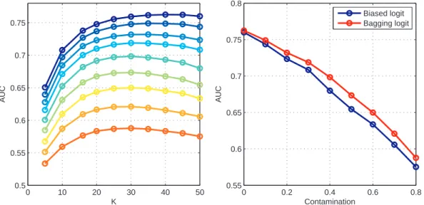
• Compare their performance on a test set of 1000 examples containing 50% positives. For K, we tested equally spaced values between 1 and 50, and we varied γ on the interval [0; 0.9]. The performance is measured by computing the area under the Receiving Operator Characteristic curve (AUC) on the independent test set. Figure 1 (left) shows the performance of bagging logit for different levels of contamination of U , as a function of K, the size of the random samples. The uppermost curve thus corresponds to γ = 0, i.e., the case where all unlabeled data are negative, while the bottom curve corresponds to γ = 0.8, i.e., the case where 80% of unlabeled data are positive. Note that K = 50 corresponds to classical bagging on the biased logit classifier, i.e., to the case where all unlabeled examples are used to train the classifier.

We observe that in the classical setting of supervised binary classification where U is not contaminated by positive samples (γ = 0), the bagging procedure does not improve performance, whatever the size of the bootstrap samples. On the other hand, as contamination increases, we observe an overall decrease of the performance, confirming that the classification problem becomes more difficult when contamination increases. In addition, the bagging logit always succeeds in reaching at least the same performance for some value of K below 50, even for high rates of contamination. Figure 1 (right) shows the evolution of AUC as γ increases, for both methods. For the bagging logit we report the AUC reached for the best K value. We see that bagging logit slightly outperforms biased logit method.

0 10 20 30 40 50 0.5 0.55 0.6 0.65 0.7 0.75 K AUC 0 0.2 0.4 0.6 0.8 0.55 0.6 0.65 0.7 0.75 0.8 Contamination AUC Biased logit Bagging logit

Figure 1: Results on simulated data. Left: AUC of the bagging logit as a function of K, the size of the bootstrap samples, on simulated data. Each curve, from top to bottom, corresponds to a contamination level γ ∈ {0; 0.1; 0.2; . . . ; 0.8}. Right Performance of two methods as a function of γ, the contamination level, on simulated data. The performance of bagging logit was taken at the optimal K value.

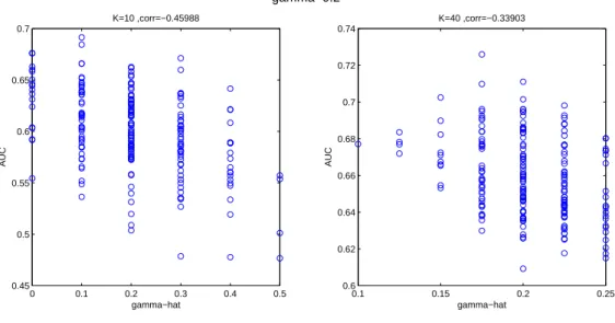
To further illustrate the assumption that motivated bagging SVM, namely that decreasing K would decrease the average performance of single classifiers but would increase their variance due to the variations in contamination, we show in Figure 2 a scatter plot of the AUC of individual classifiers as a function of the empirical contamination of the bootstrap sample ˆγ, for two values of K (10 and 40). Here the mean contamination was set to γ = 0.2. Obviously, the variations of ˆγ are much larger for K = 10 (between 0 and 0.5) than for K = 40 (between

1_{The bagging logit corresponds to the procedure described above, when the classifier is a logistic regression.}

0.1 and 0.25). The correlation coefficient between ˆγ and the performance (reported above each plot) is strongly negative, in particular for smaller K. It is quite clear that less contaminated subsamples tend to yield better classifiers, and that the variation in the contamination is an important factor to increase the variance between individual predictors, which aggregation can benefit from. 0 0.1 0.2 0.3 0.4 0.5 0.45 0.5 0.55 0.6 0.65 0.7 K=10 ,corr=−0.45988 gamma−hat AUC gamma=0.2 0.1 0.15 0.2 0.25 0.6 0.62 0.64 0.66 0.68 0.7 0.72 0.74 K=40 ,corr=−0.33903 gamma−hat AUC

Figure 2: Distribution of AUC and ˆγ over the 500 iterations of one bootstrap loop on the simulated dataset, γ = 0.2.

5.2 Newsgroup dataset

The 20 Newsgroup benchmark is widely used to test PU learning methods. The version we used is a collection of 11293 articles partitioned into 20 subsets of roughly the same size (around 500)2

, corresponding to post articles of related interest. For each newsgroup, the positive class consists of those ∼500 articles known to be relevant, while the negative class is made of the remainder. After pre-processing, each article is represented by a 8165-dimensional vector, using the TFIDF representation over a dictionnary of 8165 words (Joachims, 1997).

To simulate a PU learning problem, we applied the following strategy. For a given news-group, we created a set P of known positive examples by randomly selecting a given number of positive examples, while U contains the non-selected positive examples and all negative ex-amples. We varied the size N P of P in {5, 10, 20, 50, 100, 200, 300} to investigate the influence of the number of known positive examples. For each newsgroup and each value of N P , we train all 4 methods described above (bagging SVM, biased SVM, baseline, one-class SVM) and rank the samples in U by decreasing score (transductive setting). We then compute the area under the ROC curve (AUC), and average this measure over 10 replicates of each newsgroup and each value of N P . For bagging and biased SVM, we varied the C parameter over the grid [exp(−12 : 2 : 2)], while we vary parameter ν in [0.1 : 0.1 : 0.9] for 1-class SVM. We only used the linear kernel.

We first investigated the influence of T . Figure 3 shows, for the first newsgroup, the perfor-mance reached as a function of T , for different settings in N P and K. As expected we observe that in general the performance increases with T , but quickly reaches a plateau beyond which additional bootstraps do not improve performance. Overall the smaller K, the larger T must

2_{We used the Matlab pre-processed version available at http://renatocorrea.googlepages.com/}

be to reach the plateau. From these preliminary results we set T = 35 for K ≤ 20, and T = 10 for K > 30, and kept it fix for the rest of the experiments. To further clarify the benefits of bagging, we show in Figure 5.2 the performance of the bagging SVM versus the performance of a SVM trained on a single bootstrap sample (T = 1), for different values of K and a fixed number of positives N P = 10. We observe that, for K below 200, aggregating classifiers over several bootstrap subsamples is clearly beneficial, while for larger values of K it does not really help. This is coherent with the observation that SVM usually rarely benefit from bagging: here the benefits come from our particular bagging scheme. Interestingly, we see that very good performance is reached even for small values of K with the bagging.

5 15 25 35 45 55 65 75 85 95 105 0.78 0.79 0.8 0.81 0.82 NP=5 T AUC 5 15 25 35 45 55 65 75 85 95 105 0.84 0.845 0.85 0.855 0.86 0.865 0.87 NP=10 T AUC 5 15 25 35 45 55 65 75 85 95 105 0.87 0.875 0.88 0.885 0.89 0.895 0.9 NP=20 T AUC 5 15 25 35 45 55 65 75 85 95 105 0.9 0.91 0.92 0.93 0.94 NP=100 T AUC 5 10 20 50 100 200 500 K

Figure 3: Performance on one newsgroup as a function of the number of boostraps T , for different values of N P and K.

5 20 100 500 2050 4000 8500 0.7 0.71 0.72 0.73 0.74 0.75 0.76 0.77 0.78 0.79 0.8 K AUC Mean AUC Bagged AUC

Figure 4: Performance on one newgroup of bagging SVM (bagging AUC ) vs a SVM trained on a single bootstrap sample (mean AUC ), for different values of K.

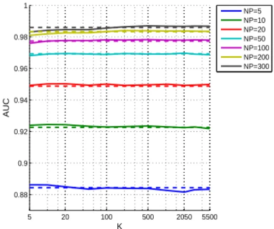
SVM as a function of K, and compares it to that of the biased SVM. More precisely, each point on the curve corresponds to the performance averaged over the 20 Newsgroups after choosing a posteriori the best C parameter for each newsgroup. This is equivalent to comparing optimal cases for both methods. Contrary to what we observed on simulated date, we observe that K has in general very little influence on the performance. The AUC of the bagging SVM is similar to that of the biased SVM for most values of K, although for N P larger than 50, a slight advantage can be observed for the biased SVM over bagging SVM when K is too small. We conclude that in practice, parameter K may not need to be finely tuned and we advocate to keep it moderate. In all cases, K = N P seems to be a safe choice for the bagging SVM.

Finally, Figure 6 shows the average AUC over the 20 newsgroups for all four methods, as a function of N P . Overall all methods are very similar, with the Baseline slightly below the others. In details, the bagging SVM curve dominates all other methods for N P ≥ 20, while the 1-class SVM is the one which dominates for smaller values of N P . Although the differences in performance are small, the bagging SVM outperforms the biased SVM significantly for N P > 20 according to a Wilcoxon paired sample test (at 5% confidence). For small values of N P however, no significant difference can be proven in either way between bagging SVM and 1-class SVM, which remains a very competitive method.

5 20 100 500 2050 5500 0.88 0.9 0.92 0.94 0.96 0.98 1 K AUC NP=5 NP=10 NP=20 NP=50 NP=100 NP=200 NP=300

Figure 5: Macro averaged performance of the bagging SVM as a function of K. The dashed horizontal lines show the AUC level of the biased SVM. The curves are plotted for different values of N P , the size of the positive set.

5.3 E. coli _{dataset : inference of transcriptional regulatory network}

In this section we test the different PU learning strategies on the problem of inferring the transcription regulatory network of the bacteria Escherichia coli from gene expression data. The problem is, given a transcription factor (TF), to predict which genes it regulates. Following Mordelet and Vert (2008), we can formulate this problem as transductive PU learning by starting from known regulated genes (considered positive examples), and looking for additional regulated genes in the bacteria’s genome.

To represent the genes, we use a compendium of microarray expression profiles provided by Faith et al. (2008), in which 4345 genes of the E. Coli genome are represented by vectors in dimension 445, corresponding to their expression level in 445 different experiments. We extracted the list of known regulated genes for each TF from RegulonDB (Salgado et al., 2006). We restrict ourselves to 31 TFs with at least 8 known regulated genes.

For each TF, we ran a double 3-fold cross validation with an internal loop on each training set to select parameter C of the SVM (or ν for the 1-class SVM). Following Mordelet and Vert (2008), we normalize the expression data to unit norm, use a Gaussian RBF kernel with σ = 8,

5 10 20 50 100 200 300 0.86 0.88 0.9 0.92 0.94 0.96 0.98 1 NP AUC Biased SVM 1class SVM Baseline Bagging

Figure 6: Performance of the baseline method, the 1-class SVM, the biased SVM and the newly proposed bagging SVM methods on the 20 Newsgroups dataset. Each curve shows how the mean AUC varies with the number of positive training examples N P . For each value of N P , the performance of bagging SVM is computed at the optimal value for K, as shown in Figure 5.

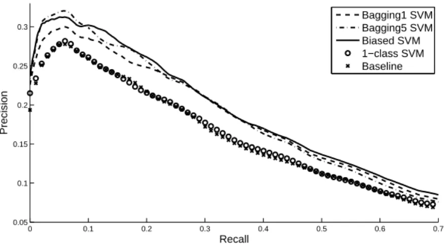
and perform a particular cross-validation scheme to ensure that operons are not split between folds. Finally, following our previous results on simulated data and the newsgroup benchmark, we test two variants of bagging SVM, setting K successively to N P and 5 ∗ N P . These choices are denoted respectively by bagging1 SVM and bagging5 SVM.

Figure 5.3 shows the average precision/recall curves of all methods tested. Overall we observe that all three PU learning methods give significantly better results than the two methods which use only positive examples (Wilcoxon paired sample test at 5% significance level). No significant difference was found between the three PU learning methods. This confirms again that for different values of K bagging SVM matches the performance of biased SVM.

0 0.1 0.2 0.3 0.4 0.5 0.6 0.7 0.05 0.1 0.15 0.2 0.25 0.3 Recall Precision Bagging1 SVM Bagging5 SVM Biased SVM 1−class SVM Baseline

Figure 7: Precision-recall curves to compare the performance between the baggin1 SVM, the bagging5 SVM, the biased SVM, the 1-class SVM and the baseline method.

6

Discussion

The main contribution of this work is to propose a new method, bagging SVM, both for inductive and transductive PU learning, and to assess in detail its performance and the influence of various

parameters on simulated and real data.

The motivation behind bagging SVM was to exploit an intrinsic feature of PU learning to benefit from classifier aggregation through a random subsample strategy. Indeed, by randomly sampling K examples from the unlabeled examples, we can expect various contamination rates, which in turn can lead to very different single classifiers (good ones when there is little con-tamination, worse ones when contamination is high). Aggregating these classifiers can in turn benefit from the variations between them. This suggests that K may play an important role in the final performance of bagging SVM, since it controls the trade-off between the mean and variance of individual classifiers. While we showed on simulated data that this is indeed the case, and that there can be some optimum K to reach the best final accuracy, the two experi-ments on real data did not show any strong influence of K and suggested that K = N P may be a safe default choice. This is a good news since it does not increase the number of parameters to optimize for the bagging SVM and leads to balanced training sets that most classification algorithms can easily handle.

The comparison between different methods is mitigated. While bagging SVM outperforms biased SVM on simulated data, they are not significantly different on the two experiments with real data. Interestingly, while these PU learning methods were significantly better than two methods that learned from positive examples only on the gene regulatory network example, the 1-class SVM behaved very well on the 20 newsgroup benchmark, even outperforming the PU learning methods when less than 10 training examples were provided. Many previous works, including Liu et al. (2003) and Yu et al. (2004) discard 1-class SVMs for showing a bad performance in terms of accuracy, while Manevitz and Yousef (2001) report the lack of robustness of this method arguing that it has proved very sensitive to changes of parameters. Our results suggest that there are cases where it remains very competitive, and that PU learning may not always be a better strategy than simply learning from positives.

Finally, the main advantage of bagging SVM over biased SVM is the computation burden, in particular when there are far more unlabeled than positive examples. Indeed, a typical algorithm, such as an SVM, trained on N samples, has time complexity proportional to Nα, with α between 2 and 3. Therefore, biased SVM has complexity proportional to (P + U )α _while

bagging SVM’s complexity is proportional T ∗ (P + K)α. With the default choice K = P ratio of CPU time to train the biased SVM vs the bagging SVM can therefore be expected to be ((P + U )/(2P ))α/T . Then we conclude that bagging SVM should be faster than biased SVM as soon as U/P > 2T1/α_{− 1. For example, taking T = 35 and α = 3, bagging SVM should}

be faster than biased SVM as soon as U/P > 6, a situation very often encountered in practice where the ratio U/P is more likely to be several orders of magnitude larger. In the two real datasets, this was always the case. Table 6 reports CPU time and performance measure for training bagging SVM on the first fold of newsgroup 1 with C fixed at its best value a posteriori and N P = 10. CPU AUC-AUP Bagging K=10 K=50 K=200 K=10 K=50 K=200 T 35 13 39 91 0.921-0.531 0.917-0.524 0.902-0.518 50 18 54 127 0.920-0.539 0.914-0.522 0.904-0.522 200 72 170 473 0.918-0.539 0.910-0.528 0.904-0.511

Table 1: CPU time and performance measures for different settings of T and K for bagging SVM.

In comparison, the biased SVM’s CPU time is 227s for AUC = 0.932 and AUP = 0.491. This confirms that for reasonable values of T and K, the bagging SVM is much faster than the biased SVM for a comparable performance.

References

Aerts et al. Gene prioritization through genomic data fusion. Nat. Biotechnol., 24(5):537–544, May 2006.

P. L. Bartlett and A. Tewari. Sparseness vs estimating conditional probabilities: Some asymp-totic results. J. Mach. Learn. Res., 8:775–790, 207.

L. Breiman. Bagging predictors. Mach. Learn., 24(2):123–140, 1996. L. Breiman. Random forests. Mach. Learn., 45(1):5–32, 2001.

Chapelle et al. Semi-Supervised Learning. MIT Press, Cambridge, MA, 2006.

De Bie et al. Kernel-based data fusion for gene prioritization. Bioinformatics, 23(13):i125–i132, Jul 2007.

Denis et al. Learning from positive and unlabeled examples. Theoretical Computer Science, 348 (1):70–83, 2005.

C. Elkan and K. Noto. Learning classifiers from only positive and unlabeled data. In KDD ’08:

Proceeding of the 14th ACM SIGKDD international conference on Knowledge discovery and data mining, pages 213–220, New York, NY, USA, 2008. ACM.

Faith et al. Many microbe microarrays database: uniformly normalized affymetrix compendia with structured experimental metadata. Nucleic Acids Res, 36(Database issue):D866–D870, Jan 2008.

Hastie et al. The elements of statistical learning: data mining, inference, and prediction. Springer, 2001.

T. Joachims. Transductive inference for text classification using support vector machines. In

ICML ’99: Proceedings of the Sixteenth International Conference on Machine Learning, pages

200–209, San Francisco, CA, USA, 1999. Morgan Kaufmann Publishers Inc. ISBN 1-55860-612-2.

T. Joachims. A probabilistic analysis of the rocchio algorithm with TFIDF for text catego-rization. In ICML ’97: Proceedings of the Fourteenth International Conference on Machine

Learning, pages 143–151, Nashville, Tennessee, USA, 1997. Morgan Kaufmann Publishers

Inc.

W. S. Lee and B. Liu. Learning with positive and unlabeled examples using weighted logistic regression. In T. Fawcett and N. Mishra, editors, Machine Learning, Proceedings of the

Twentieth International Conference (ICML 2003, pages 448–455. AAAI Press, 2003.

X. Li and B. Liu. Learning to classify texts using positive and unlabeled data. In IJCAI’03:

Proceedings of the 18th international joint conference on Artificial intelligence, pages 587–592,

San Francisco, CA, USA, 2003. Morgan Kaufmann Publishers Inc.

Liu et al. Partially supervised classification of text documents. In ICML ’02: Proceedings of

the Nineteenth International Conference on Machine Learning, pages 387–394, San Francisco,

CA, USA, 2002. Morgan Kaufmann Publishers Inc. ISBN 1-55860-873-7.

Liu et al. Building text classifiers using positive and unlabeled examples. In Intl. Conf. on Data

Mining, pages 179–186, 2003.

L. M. Manevitz and M. Yousef. One-class SVMs for document classification. J. Mach. Learn.

F. Mordelet and J.-P. Vert. Sirene: Supervised inference of regulatory networks. Bioinformatics, 24(16):i76–i82, 2008.

K. Pelckmans and J.A.K. Suykens. Transductively learning from positive examples only. In

Proc. of the European Symposium on Artificial Neural Networks (ESANN 2009), 2009.

Salgado et al. RegulonDB (version 5.0): Escherichia coli K-12 transcriptional regulatory net-work, operon organization, and growth conditions. Nucleic Acids Res., 34(Database issue): D394–D397, Jan 2006.

Sch¨olkopf et al. Estimating the Support of a High-Dimensional Distribution. Neural Comput., 13:1443–1471, 2001.

C. Scott and G. Blanchard. Novelty detection: Unlabeled data definitely help. In D. van Dyk and M. Welling, editors, Proceedings of the Twelfth International Conference on Artificial

Intelligence and Statistics (AISTATS) 2009, volume 5, pages 464–471, Clearwater Beach,

Florida, 2009. JMLR: W&CP 5.

Shah et al. SVM-HUSTLE–an iterative semi-supervised machine learning approach for pairwise protein remote homology detection. Bioinformatics, 24(6):783–790, Mar 2008.

Sriphaew et al. Cool blog classification from positive and unlabeled examples. Advances in

Knowledge Discovery and Data Mining, pages 62–73, 2009.

I. Steinwart. Sparseness of Support Vector Machines. J. Mach. Learn. Res., 4:1071–1105, 2003. R. Vert and J.-P. Vert. Consistency and convergence rates of one-class SVMs and related

algorithms. J. Mach. Learn. Res., 7:817–854, 2006.

Yu et al. PEBL: Web page classification without negative examples. IEEE Trans. Knowl. Data

Eng., 16(1):70–81, 2004.

C. C. Chang and C. J. Lin. LIBSVM: a library for support vector machines, 2001. Software available at http://www.csie.ntu.edu.tw/~cjlin/libsvm.

Zhang et al. Maximum margin clustering made practical. IEEE T. Neural Network, 20(4): 583–596, 2009.