Dynamic Models of R&D, Innovation and Productivity: Panel Data Evidence for Dutch and French Manufacturing

(1)

Montréal

Mai 2013

© 2013 Wladimir Raymond, Jacques Mairesse, Pierre Mohnen, Franz Palm. Tous droits réservés. All rights reserved. Reproduction partielle permise avec citation du document source, incluant la notice ©.

Short sections may be quoted without explicit permission, if full credit, including © notice, is given to the source.

Série Scientifique

Scientific Series

2013s-12

Dynamic Models of R&D, Innovation and Productivity:

Panel Data Evidence for Dutch and French Manufacturing

(2)

CIRANO

Le CIRANO est un organisme sans but lucratif constitué en vertu de la Loi des compagnies du Québec. Le financement de son infrastructure et de ses activités de recherche provient des cotisations de ses organisations-membres, d’une subvention d’infrastructure du Ministère du Développement économique et régional et de la Recherche, de même que des subventions et mandats obtenus par ses équipes de recherche.

CIRANO is a private non-profit organization incorporated under the Québec Companies Act. Its infrastructure and research activities are funded through fees paid by member organizations, an infrastructure grant from the Ministère du Développement économique et régional et de la Recherche, and grants and research mandates obtained by its research teams.

Les partenaires du CIRANO Partenaire majeur

Ministère de l'Enseignement supérieur, de la Recherche, de la Science et de la Technologie Partenaires corporatifs

Autorité des marchés financiers Banque de développement du Canada Banque du Canada

Banque Laurentienne du Canada Banque Nationale du Canada Banque Scotia

Bell Canada

BMO Groupe financier

Caisse de dépôt et placement du Québec Fédération des caisses Desjardins du Québec Financière Sun Life, Québec

Gaz Métro Hydro-Québec Industrie Canada Investissements PSP

Ministère des Finances et de l’Économie Power Corporation du Canada

Rio Tinto Alcan

State Street Global Advisors Transat A.T.

Ville de Montréal

Partenaires universitaires École Polytechnique de Montréal École de technologie supérieure (ÉTS) HEC Montréal

Institut national de la recherche scientifique (INRS) McGill University

Université Concordia Université de Montréal Université de Sherbrooke Université du Québec

Université du Québec à Montréal Université Laval

Le CIRANO collabore avec de nombreux centres et chaires de recherche universitaires dont on peut consulter la liste sur son site web.

ISSN 1198-8177

Les cahiers de la série scientifique (CS) visent à rendre accessibles des résultats de recherche effectuée au CIRANO afin de susciter échanges et commentaires. Ces cahiers sont écrits dans le style des publications scientifiques. Les idées et les opinions émises sont sous l’unique responsabilité des auteurs et ne représentent pas nécessairement les positions du CIRANO ou de ses partenaires.

This paper presents research carried out at CIRANO and aims at encouraging discussion and comment. The observations and viewpoints expressed are the sole responsibility of the authors. They do not necessarily represent positions of CIRANO or its partners.

(3)

Dynamic Models of R&D, Innovation and Productivity:

Panel Data Evidence for Dutch and French Manufacturing

*

Wladimir Raymond

†

, Jacques Mairesse

‡

, Pierre Mohnen

§

, Franz Palm

**

Résumé / Abstract

Dans ce papier, nous introduisons de la dynamique dans le modèle Crépon-Duguet-Mairesse (CDM), à

la fois entre la R-D et l’innovation et entre l’innovation et la productivité. Le modèle CDM a

généralement été estimé sur des données en coupe transversale. Nous proposons quatre modèles

dynamiques à équations simultanées avec des effets individuels et des effets idiosyncratiques corrélés

entre équations. Ces modèles diffèrent dans la façon dont l’innovation apparaît dans l’équation de

productivité : à travers une variable binaire ou une variable continue, et à travers une mesure observée

ou une mesure latente de l’innovation. Les modèles sont estimés par maximum de vraisemblance sur

des données panel d’entreprises françaises et néerlandaises provenant de trois vagues des enquêtes

communautaires d’innovation. Les résultats sont robustes et montrent que la causalité est

unidirectionnelle allant de l’innovation à la productivité, et que la persistance est plus forte dans la

productivité que dans l’innovation.

Mots clés : R-D, innovation, productivité, données panel, dynamique, équations

simultanées.

This paper introduces dynamics in the R&D to innovation and innovation to productivity

relationships, which have mostly been estimated on cross-sectional data. It considers four nonlinear

dynamic simultaneous equations models that include individual effects and idiosyncratic errors

correlated across equations and that differ in the way innovation enters the conditional mean of labor

productivity: through an observed binary indicator, an observed intensity variable or through the

continuous latent variables that correspond to the observed occurrence or intensity. It estimates these

models by full information maximum likelihood using two unbalanced panels of Dutch and French

manufacturing firms from three waves of the Community Innovation Survey. The results provide

evidence of robust unidirectional causality from innovation to productivity and of stronger persistence

in productivity than in innovation.

Keywords: R&D, Innovation, Productivity, Panel data, Dynamics, Simultaneous

equations.

Codes JEL: C33, C34, C35, L60, O31, O32.

*

The authors wish to thank the participants of the various seminars where this paper has been presented for their comments and suggestions, in particular St´ephane Robin, Ulya Ulku and Adrian Wood.

†_{STATEC, wladimir.raymond@statec.etat.lu.} ‡

CREST-INSEE, UNU-MERIT, Maastricht University and NBER; mairesse@ensae.fr

§_{Corresponding author: UNU-MERIT, Maastricht University and CIRANO, University of Maastricht, P.O.} Box 616, 6200 MD Maastricht, The Netherlands; Tel.: (+31) 43 388 4464; Fax: (+31) 43 388 4905

p.mohnen@maastrichtuniversity.nl **

(4)

1 Introduction

For decades, R&D and innovation have been recognized by scholars and policy makers as major drivers of country, industry and firm economic performance. Many of the early studies, follow-ing the lead ofGriliches (1979), have used an augmented production function with R&D capital to estimate the returns to R&D at the firm level. More recently, many studies have relied on innovation survey indicators and on the CDM framework to analyze simultaneously a knowledge production function relating innovation output to R&D, and an augmented production function linking productivity to innovation output (Crépon et al.,1998;Mairesse et al.,2005;Griffith et al., 2006). Both the effects of R&D on innovation output and of innovation output on productivity are usually found to be positive and significant in these studies. Most of them, however, are based on cross-sectional data and cannot take into account the dynamic linkages between innovation and economic performance nor unobserved firm heterogeneity. This is where the present study comes into play.1 More specifically, using data from three waves of the Community Innovation Survey (CIS) for France and the Netherlands, we examine whether there is evidence of persistence in firm innovation and productivity and of bidirectional causality between them.

There are several reasons why one should introduce dynamics in the interrelationships between R&D, innovation and productivity. Firstly, the time lag between a firm’s decision to invest in R&D, the associated R&D outlays and the resulting innovation success may be substantial because of ‘time to build’, opportunity cost and uncertainty inherent to the innovation process (Majd and Pindyck, 1987). For example, the studies of knowledge production function on firm panel data, where patents proxy for knowledge, specify a relation of patents to distributed lags of R&D (Pakes and Griliches,1980;Hall et al.,1986). Secondly, scholars argue that a successfully innovative firm is more likely than a non-innovating firm to experience innovation success in the future, in other words, that ‘success breeds success’. Several papers have investigated the persistence of innovation success, measured by the number of granted patents (Geroski et al., 1997), the introduction of new or significantly improved products (Peters,2009) or production methods (Flaig and Stadler, 1994), or the share in total sales accounted for by sales of these products (henceforth the share of innovative sales) (Raymond et al.,2010). Thirdly, it is also argued that the economic performance of a firm, especially of a repeatedly innovating firm, is likely to exhibit persistence. For instance, Bailey et al.(1992), Bartelsman and Dhrymes(1998), andFariñas and Ruano(2005) find strong evidence of persistence of firm level productivity differentials using transition probabilities on the quintiles or deciles of the distribution of these differentials over time, or using kernel techniques

(5)

to estimate the conditional distribution of firm level productivity at period t given productivity at period t− 1. Finally, because of information asymmetry, firms may be more willing to rely on retained earnings rather than to seek external funding for their future innovations (Bhattacharya and Ritter,1983), implying a feedback effect from productivity to innovation.

To investigate these dynamic aspects, we study four nonlinear dynamic simultaneous equations models that diﬀer in the way that innovation enters the conditional mean of labor productivity: through an observed binary indicator, an observed intensity variable or through the continuous latent variables that correspond to the observed occurrence or intensity. We describe these models in detail in Section2.

We show in Section3how to derive the full information maximum likelihood estimator assum-ing random effects that are correlated with sufficiently time-varyassum-ing explanatory variables. More specifically, we take care of the initial conditions problem due to the autoregressive structure of the models and the presence of firm effects usingWooldridge’s (2005) ‘simple solutions’ approach, and we handle multiple integration due to the correlations of firm effects and idiosyncratic errors across equations using Gauss-Hermite quadrature sequentially along the lines ofRaymond (2007, chapter 6).

In Section4, we explain the data on which we base our estimations and provide some descrip-tive statistics. These data come from three waves of the Dutch and the French Manufacturing Community Innovation Surveys (CIS) for 1994-1996, 1998-2000 and 2002-2004, supplemented by a few ﬁrm accounting variables. We work with an unbalanced panel to have a larger sample and thus to weaken possible survivorship biases and to obtain more accurate estimates.

In Section5we present our results. For both countries they reveal strong persistence in produc-tivity but weaker persistence in innovation, and they indicate a unidirectional causality running from innovation to labor productivity. Whereas past innovation matters to productivity, the most productive enterprises are not more successful in introducing new or signiﬁcantly improved prod-ucts and do not attain larger shares of innovative sales than the least productive ones.

2 Model speciﬁcations

Our models consist of a knowledge production function and an augmented production function relating respectively innovation output to R&D and other relevant innovation factors, and pro-ductivity to innovation output and other relevant production factors. Four variables of innovation output are considered in the analysis. The ﬁrst is an observed binary variable taking the value one if an enterprise is a product innovator, and zero otherwise. In the innovation survey, an enterprise

(6)

is asked whether it has introduced at least one new or improved product on the market in the last three years. A product innovator is an enterprise that has responded positively to this question. The second variable is the observed share of innovative sales, or observed innovation intensity. This variable is directly reported by the enterprise when ﬁlling out the questionnaire of the innovation survey. The share of innovative sales is taken with respect to sales reported in the last year of the three-year period. Finally we consider the two continuous latent innovation output variables that underly respectively the propensity to introduce new or improved products on the market and the potential share of innovative sales.

2.1 Knowledge production function (KPF)

Let y∗_1it denote a latent variable underlying ﬁrm i’s (i = 1, ..., N ) propensity to achieve product innovations at period t (t = 0i, ..., Ti) given past observed occurrence of product innovations y1i,t−1,

past labor productivity y3i,t−1, past R&D and other ﬁrm- and market-speciﬁc characteristics x1it,

and unobserved ﬁrm heterogeneity α1i.2 Formally

y_1it∗ = ϑ11y1i,t−1+ ϑ13y3i,t−1+ β′1x1it+ α1i+ ε1it, (2.1)

where ϑ11 and ϑ13capture the eﬀect of past product innovation occurrence and past productivity

on the propensity to innovate, β′₁captures the eﬀects of past R&D and other explanatory variables and ε1it denotes idiosyncratic errors encompassing other time-varying unobserved variables that

aﬀect y_1it∗ . The observed dependent variable, y1it, corresponding to y∗1itis deﬁned as

y1it= 1[y1it∗ > 0], (2.2)

where 1[ ] denotes the indicator function taking the value one if the condition between squared brackets is satisﬁed, and zero otherwise.

Let y∗_2it denote the ﬁrm’s latent share of innovative sales, or potential innovation intensity, given past observed innovation intensity y2i,t₋₁, past labor productivity y3i,t₋₁, past R&D and

other firm- and market-specific characteristics x2it, and firm-specific effects α2i. Formally

y2it∗ = ϑ22y2i,t−1+ ϑ23y3i,t−1+ β′2x2it+ α2i+ ε2it, (2.3)

where the coeﬃcients ϑ22and ϑ23capture the eﬀect of past observed share of innovative sales and 2_{By letting t vary from 0}

ito Ti, we allow firms to enter and exit the sample at different periods. 0idenotes the first observation of firm i in the unbalanced panel data sample and Tiits last observation.

(7)

past labor productivity on the potential innovation intensity, β′₂ captures the eﬀect of past R&D and other explanatory variables and ε2it denotes idiosyncratic errors. The observed counterpart

to y_2it∗ is deﬁned as

y2it= 1[y∗1it> 0]y2it∗ . (2.4)

In other words, the share of innovative sales of ﬁrm i is observed to be positive in period t if its innovation propensity is suﬃciently large in that period. If not, the share of innovative sales is set equal to zero.

The product innovation indicator and the share of innovative sales variables are taken from the innovation survey of the two countries. Since the share of innovative sales lies within the unit interval, we use a logit transformation in the estimation in order to normalize it over the entire set of real numbers.3

The set of other explanatory variables includes the log R&D per employee, the log market share, and size, industry and time dummy variables.4 Due to the lengthy nature of research and innovation activities, we use lagged R&D to explain innovation occurrence and innovation intensity. Since we cannot construct a stock measure of R&D, we restrict ourselves to R&D expenditures of continuous R&D performers. We include a lagged dummy variable for non-continuous R&D performers to compensate for the fact that we use positive values of R&D only for continuous R&D performers. Market share is used at the three digit industry level as a measure of relative size that can reflect market power. It is lagged in order to avoid possible endogeneity concerns (due in particular to measurement errors in firm sales which would affect both our market share and productivity variables).5 _{We take employment as our measure of firm absolute size, and}

since the relation between innovation and size may be nonlinear, we use four size class indicators: small enterprises (# employees≤ 50), medium-sized enterprises (50 < # employees ≤ 250), large enterprises (250 < # employees ≤ 500) and very large enterprises (500 < # employees), the fourth class being considered as the reference. We control for industry effects, according to the OECD (2007) technology-based classification of high-tech, medium-high-tech, medium-low-tech, and low-tech industries, using three dummy variables for the first three industry categories and taking low-tech industries as the reference. Such industry-specific effects capture differences in technological opportunities (it is easier to innovate in certain industries than in others) and in

3_{Zero values of the share of innovative sales are replaced by a positive value τ}

1smaller than the minimum positive

observed value of that variable, and values one are replaced by a positive value τ2 higher than the second largest

observed value. These choices have a negligible eﬀect on our estimates.

4_{In some speciﬁcations, we have also three indicators of the distance to the productivity frontier. We ﬁnd,}

however, that they are not statistically signiﬁcant (see AppendixD).

5_{The market share of a ﬁrm is deﬁned as the ratio of its sales over the total sales of the three digit industry it}

belongs to. The latter is obtained by adding up the sales of all ﬁrms in our sample that belong to that industry after multiplying them by the appropriate raising factor.

(8)

intensity of competition (which is expected to be higher in high-tech than in low-tech industries). Since our panel consists only of three periods and we need one for the lagged variables, we need only include a time dummy variable for the period 1998-2000, with 2002-2004 being the reference. This time dummy controls for macroeconomic shocks and for inﬂation.

2.2 Augmented production function (APF)

As in the great majority of studies, we assume a Cobb-Douglas APF that we write in terms of a log linear productivity equation relating labor productivity to labor (i.e., we do not assume a constant scale elasticity), physical capital per employee (proxied here by physical investment due to the unavailability of a stock measure), and innovation output. We consider four specifications where we explain productivity by latent innovation (i.e. the propensity to achieve product innovations or potential innovation intensity) or by observed innovation (i.e. innovation occurrence or observed innovation intensity). In all cases we also condition current labor productivity on its past values and control for unobserved heterogeneity through firm effects. Thus, we can write

y3it= ϑ33y3i,t−1+ β′3x3it+ γjy∗jit+ α3i+ ε3it, (2.5a)

y3it= ϑ33y3i,t−1+ β′3x3it+ γjyjit+ α3i+ ε3it, (2.5b)

with j = 1 or 2 where innovation propensity (y∗_1it) or potential innovation intensity (y∗_2it) explains labor productivity in equation (2.5a), and innovation occurrence (y1it) or observed innovation

intensity (y2it) explains labor productivity in equation (2.5b). The coeﬃcient ϑ33 captures the

effect of past labor productivity on current labor productivity, β′₃ captures the effect of standard input variables, i.e. employment and physical investment per employee, γj captures the effect of

innovation output on labor productivity, and α3i and ε3it denote time-invariant ﬁrm eﬀects and

idiosyncratic errors. We also control for industry and time eﬀects as in the KPF equations.

3 Full information maximum likelihood estimation (FIML)

We shall now explain how to derive the FIML estimator, that is how to take care of the initial conditions problem due to the autoregressive structure of the models and the presence of firm effects, how to write the likelihood function, and how to handle the multiple integration due to the correlations of firm effects and idiosyncratic errors across equations.

(9)

3.1 Initial conditions

The initial conditions problem stems from the fact that the first observed value of the lagged dependent variables is correlated with the individual effects. Ignoring or inadequately accounting for this correlation results in a bias of the effect of the lagged dependent variables. Several solutions have been proposed in the econometric literature. We follow the one suggested by Wooldridge (2005).

Wooldridge’s ‘simple solutions’ have been originally applied to autoregressive nonlinear single-equation models with individual effects. We adapt the approach to a model with multiple single-equations. In other words, we project in each equation the individual effects on the first observation of the corresponding dependent variables and on the observed history of the explanatory variables. Formally α1i = b10+ b′11y1i0i+ b ′ 12x1i+ a1i, (3.1) α2i = b20+ b′21y2i0i+ b ′ 22x2i+ a2i, (3.2) α3i = b30+ b′31y3i0i+ b ′ 32x3i+ a3i, (3.3)

where y_ki0_i (k = 1, 2, 3) represents the initial values of the dependent variables, xki= (xki0i+1, ...,

xkiT_i)′ represents the history of (in principle all) the observations of the time-varying explanatory variables, and ai = (a1i, a2i, a3i)′ denotes the vector of projection errors assumed orthogonal to

y_ki0_i, xkiand εit= (ε1it, ε2it, ε3it)′. The ancillary parameters bk0, bk1and bk2are to be estimated

alongside the parameters of interest.

Three important remarks are in order regarding equations (3.1)-(3.3). Firstly, if the coeﬃcient vectors β_k contain intercepts, only the sums of those intercepts and bk0 are identiﬁed. Secondly,

if the explanatory variables are time-invariant or do not show sufficient within variation, then the coefficients bk2 and βk cannot be separately identified. As a result, only the sufficiently

time-varying explanatory variables enter equations (3.1)-(3.3). Thirdly, in order to discriminate between the effect of the lagged dependent variables and that of the initial values, given the unbalancedness of the panel, we actually have to include in equations (3.1)-(3.3) two types of initial values with different coefficients for firms present in all three waves and for those present only in two waves. FollowingWooldridge(2005) we make the following distributional assumptions:

(10)

εit_|y_i,t−1,xit,αi

iid

∼ Normal(0, Σε); ai_|y_i0i,xi

iid

∼ Normal(0, Σa) where Σε and Σaare given by

Σε=       1 ρ_ε1ε2σε2 σ 2 ε2 ρ_ε1ε3σε3 ρε2ε3σε2σε3 σ 2 ε3      , Σa=       σa21 ρa1a2σa1σa2 σ 2 a2 ρa1a3σa1σa3 ρa2a3σa2σa3 σ 2 a3       (3.4)

and are also to be estimated.

3.2 Likelihood

We now derive the likelihood functions. For simplicity, we provide the expressions explicitly only for the speciﬁcations where y_1it∗ or y1it (respectively the latent propensity to achieve product

innovations and the observed indicator of innovation occurrence) enters the augmented production function. Those with y_2it∗ or y2it are presented in AppendixB.

Model with latent innovation propensity

The model with latent innovation propensity as a predictor of labor productivity consists of equations (2.1)-(2.4) and (2.5a) with j = 1 in equation (2.5a). These equations constitute the structural form of the model. Since y_1it∗ is unobserved, we cannot, unlike in simultaneous equa-tions models with observed explanatory variables, derive the likelihood function directly where the dependent variable is included as a regressor. As a result, FIML estimates can be obtained only through the likelihood function of the reduced form of the model. The reduced-form equations are given by equations (2.1)-(2.4) and

y3it= ϑ33y3i,t−1+β′3x3it+γ1

[

ϑ11y1i,t−1+ ϑ13y3i,t−1+ β′1x1it

] +γ_|1α1i_{z+ α3i_} α3i + γ_|1ε1it_{z+ ε3it_} ϵ3it , (3.5)

where y∗_1ithas been replaced by its right-hand side expression of equation (2.1).6 _{The individual}

eﬀects and the idiosyncratic errors of the reduced form are given by αi = (α1i, α2i, α3i)′ and

εit = (ε1it, ε2it, ε3it)′, where α3i and ε3it are deﬁned in equation (3.5). After replacing α1i, α2i

and α3i by their expressions (3.1) to (3.3) into equations (2.1), (2.3) and (3.5), we obtain the

projection errors of the reduced form as ai = (a1i, a2i, a3i)′ with a3i = γ1a1i + a3i. Since the

structural form idiosyncratic errors and projection errors are both normally distributed, their reduced-form counterparts are also normally distributed with means zero and covariance matrices

6_{In the econometric literature on simultaneous equations models, equation (}_3.5_{) is referred to as restricted reduced}

form when written with all the parameters of the structural form and unrestricted reduced form when written with the underlined parameters. In the latter case, γ1ϑ11 would constitute a new coeﬃcient, say ϑ11. The restricted

(11)

Σε and Σa given by Σε=       1 ρ_ε1ε2σε2 σ 2 ε2 ρ_ε1ε3σε3 ρε2ε3σε2σε3 σ 2 ε3      , Σa=       σ_a2₁ ρa1a2σa1σa2 σ 2 a2 ρa1a3σa1σa3 ρa2a3σa2σa3 σ 2 a3      , (3.6)

where the underlined components of Σε and Σa are nonlinear functions of their structural form

counterparts and are given by

σ2_ε₃ = γ2₁+ σ_ε2₃+ 2γ1ρ_ε1ε3σε3, σ 2 a3 = γ 2 1σ 2 a1+ σ 2 a3+ 2γ1ρa1a3σa1σa3, (3.7a) ρ_ε1ε3 = ₍ γ1+ ρε1ε3σε3 γ2 1+ σ2ε3+ 2γ1ρε1ε3σε3 )1 2 , ρa1a3 = γ1σa1+ ρa1a3σa3 ( γ2 1σa21+ σ 2 a3+ 2γ1ρa1a3σa1σa3 )1 2 , (3.7b) ρ_ε2ε3 = γ1ρε1ε2+ ρε2ε3σε3 ( γ2 1+ σ2ε3+ 2γ1ρε1ε3σε3 )1 2 , ρa2a3 = γ1ρa1a2σa1+ ρa2a3σa3 ( γ2 1σa21+ σ 2 a3+ 2γ1ρa1a3σa1σa3 )1 2 . (3.7c)

The individual likelihood function of the reduced form conditional on ai, denoted by l1i|ai, is

given by l1i_|ai= Ti ∏ t=0i+1 [∫ −(A1it+a1i) −∞ ∫ _∞ −∞

h3(ε1it, ε2it, y3it)dε1itdε2it

]1−y1it

(3.8) [∫ _∞

−(A1it+a1i)

h3(ε1it, y2it, y3it)dε1it

]y1it

,

where h3 denotes the density function of the trivariate normal distribution and A1it is deﬁned as

A1it≡ ϑ11y1i,t−1+ ϑ13y3i,t−1+ β′1x1it+ b10+ b′11y1i0i+ b

′

12x1i. (3.9)

The ﬁrst product in equation (3.8) represents the contribution of a non-product innovator to the likelihood function and can be rewritten as h1(y3it)

∫ _−(A1it+a1i)

−∞

h1(ε1it|y3it)dε1it.7 The second

product represents the contribution of a product innovator and is equal to h1( y2it| y3it) h1( y3it)

∫ _∞

−(A1it+a1i)

h1(ε1it|y2it, y3it)dε1it. These single integrals are univariate cumulative distribution

functions (CDFs) of the normal distribution, and are shown to be respectively (seeKotz et al.,

7

∫ _∞

−∞h3(ϵ1it, ϵ2it, y3it)dϵ2it= h2(ϵ1it, y3it) where h2 denotes the density of the bivariate normal distribution, and h2(ϵ1it, y3it) = h1(y3it)h1(ϵ1it|y3it) where h1denotes the density of the univariate normal distribution.

(12)

2000)

Φ1



−A1it− a1i− ρε1ε3 σε−13 (y3it− A3it− γ1A1it− a3i)

√ 1− ρ2 ε1ε3   , (3.10a) Φ1 

A1it+ a1i+ ρ12.3σε−12 (y2it− A2it− a2i) + ρ13.2 σ−1ε3 (y3it− A3it− γ1A1it− a3i)

√ 1− R2

1.23



, (3.10b)

where A1itis given in equation (3.9), A2itand A3itare given by

A2it≡ ϑ22y2i,t−1+ ϑ23y3i,t−1+ β′2x2it+ b20+ b′21y2i0i+ b

′

22x2i, (3.11a)

A3it≡ ϑ33y3i,t₋₁+ β′3x3it+ b30+ b′31y3i0i+ b

′ 32x3i, (3.11b) and ρ_12.3, ρ_13.2, and R2 1.23 are given by ρ12.3 ≡ ρε1ε2−ρε1ε3 ρε2ε3 1−ρ2 ε2ε3 , ρ13.2 ≡ ρε1ε3−ρε1ε2 ρε2ε3 1−ρ2 ε2ε3 , R2_1.23≡ ρ2ε1ε2+ρ 2 ε1ε3− 2ρε1ε2 ρε1ε3 ρε2ε3 1−ρ2 ε2ε3 . (3.12) The ﬁnal expression of l1i|ai is given by

l1i|ai= Ti ∏ t=0i+1 1 σε3 ϕ1 (

y3it−A3it−γ1A1it−a3i

σε3

) Φ1



−A1it−a1i−ρε1ε3 σ−1ε3(y3it−A3it−γ1A1it−a3i)

√ 1− ρ2 ε1ε3     1−y1it  Φ1 

A1it+ a1i+ ρ12.3σ−1ε2 (y2it− A2it− a2i) + ρ13.2 σ−1ε3(y3it− A3it− γ1A1it− a3i)

√ 1− R2 1.23   (3.13) 1 σε2 √ 1− ρ2 ε2ε3 ϕ1    y2it− A2it− a2i− ρ_ε2ε3σ_ε2

σ_ε3 (y3it− A3it− γ1A1it− a3i)

σε2 √ 1− ρ2 ε2ε3       y1it .

Model with observed innovation incidence

The model with the observed innovation indicator as a predictor of labor productivity consists of equations (2.1)-(2.4) and (2.5b) with j = 1 in equation (2.5b). Unlike in the previous model, we insert directly the observed innovation indicator in the likelihood function.8

8_{As a matter of fact, adopting this approach is recommended in this case. Indeed, the indicator function that}

relates the observed dependent variable, y1it, to the regressors, which would be used in the likelihood function of

(13)

The individual likelihood function of the structural form of this model, conditional on ai and

denoted by l2i_|ai, has a similar expression to l1i|ai. It is given by

l2i|ai= Ti ∏ t=0i+1 1 σε3 ϕ1 (

y3it−A3it−γ1y1it−a3i

σε3

) Φ1



−A1it−a1i−ρ_ε1ε3_√σ−1ε3(y3it−A3it−γ1y1it−a3i)

1− ρ2 ε1ε3     1−y1it [ Φ1 (

A1it+ a1i+ ρ12.3σε−12 (y2it− A2it_√− a2i) + ρ13.2 σ−1ε3(y3it− A3it− γ1y1it− a3i)

1− R2 1.23 ) (3.14) 1 σε2 √ 1− ρ2 ε2ε3 ϕ1  y2it− A2it− a2i− ρ_ε2ε3σ_ε2

σ_ε3 (y3it− A3it− γ1y1it− a3i)

σε2 √ 1− ρ2 ε2ε3     y1it , where ρ_12.3, ρ_13.2, and R2

1.23 are derived straightforwardly from equation (3.12) by replacing the

underlined correlations by their structural form counterparts, that is

ρ12.3 ≡ ρε1ε2−ρε1ε3 ρε2ε3 1−ρ2 ε2ε3 , ρ13.2 ≡ ρε1ε3−ρε1ε2 ρε2ε3 1−ρ2 ε2ε3 , R2_1.23≡ ρ 2 ε1ε2+ρ 2 ε1ε3− 2ρε1ε2 ρε1ε3 ρε2ε3 1−ρ2 ε2ε3 . (3.15)

3.3 Numerical evaluation

The next step consists in obtaining the unconditional counterparts to l1i|ai and l2i|ai, which are

obtained by integrating out respectively ai and aiwith respect to their normal distribution.

For-mally, l1= N ∏ i=1 ∫ a1i ∫ a2i ∫ a3i l1i|aih3(a1i, a2i, a3i|...)da1ida2ida3i, (3.16) and l2= N ∏ i=1 ∫ a1i ∫ a2i ∫ a3i l2i_|aih3(a1i, a2i, a3i|...)da1ida2ida3i. (3.17)

Evidently, l1 and l2 cannot be derived analytically. Hence, we use Gauss-Hermite quadrature

sequentially, along the lines of Raymond (2007), to evaluate the triple integrals.9 _The

Gauss-Hermite quadrature states that

∫ _∞ −∞ e−r2f (r)dr≃ M ∑ m=1 wmf (am), (3.18)

where wm and am are respectively the weights and abscissae of the quadrature with M being the

total number of integration points.10 Numerical tables with values of wm and am are formulated

in mathematical textbooks (Abramowitz and Stegun,1964). The larger M , the more accurate the

9_{The use of this numerical method is well documented in the econometric literature in the context of panel data}

single-equation models (see e.g.Butler and Moﬃtt,1982;Rabe-Hesketh et al.,2005). However, its use in the context of panel data models with multiple equations remains to date limited. A few exceptions areRaymond(2007, chapter 3) who studies the performance of the method in two types of dynamic sample selection models, andRaymond et al.

(2010) who apply the method to estimate the persistence of innovation incidence and innovation intensity.

10_{The abscissae of the quadrature, a}

(14)

approximation. Using the results of AppendixA, the unconditional likelihood, l1, is derived as l1≃ N ∏ i=1 ∆π−32 [ (1− ρ2a1a2)(1− ρ 2 a1a3)(1− ρ 2 a1a2) ]−1 2 M3 ∑ m3=1 wm3 Ti ∏ t=0i+1 1 σε3 ϕ1 (

y3it− A3it− γ1A1it− am3[...]

σε3 ) M2 ∑ m2=1 wm2e −2Λ23am√ 2am3 Λ22 Λ33 Ti ∏ t=0i+1    1 σε2 √ 1− ρ2 ε2ε3 ϕ1   

y2it−A2it−am2[...]−

ρ

ε2ε3σε2

σ_ε3 (y3it−A3it−γ1A1it−am3[...])

σε2 √ 1− ρ2 ε2ε3       y1it (3.19) M1 ∑ m1=1 wm1e −2am_√ ₁ Λ11 ( am2 Λ12_√ Λ22+ am3 Λ13_√ Λ33 ) Ti ∏ t=0i+1  Φ1 

−A1it−am1[...]−ρε1ε3 σ−1ε3(y3it−A3it−γ1A1it−am3[...])

√ 1− ρ2 ε1ε3     1−y1it  Φ1 

A1it+ am1[...] + ρ12.3σε−12 (y2it−A2it−am2[...]) + ρ13.2 σ−1ε3(y3it− A3it−γ1A1it− am3[...])

√ 1− R2 1.23     y1it ,

where wmk, amk and Mk (k = 1, 2, 3) are respectively the weights, abscissae and total number of

points of the quadrature in each stage, amk[...] =

a_mk_√σ_ak√2 Λkk

, and the expressions of Λkl(k, l = 1, 2, 3;

Λkl = Λlk) and ∆ are given in AppendixA. The FIML estimates of the structural parameters of

the model where y_1it∗ enters the APF are obtained by maximizing ln l1 subject to the constraints

deﬁned in equations (3.7a)-(3.7c).

The evaluation of l2is done in a similar fashion and yields a similar expression except that the

underlined parameters are replaced by their non-underlined equivalents and that γ1A1itis replaced

by γ1y1it. The FIML estimates of the structural parameters of the model where y1it enters the

APF are obtained by maximizing ln l2 without additional constraints.

4 Data and descriptive statistics

The data used in the analysis stem from three waves of the Dutch and the French CIS pertaining to the manufacturing sector, with the exception of the food industry, for the periods 1994-1996 (CIS 2), 1998-2000 (CIS 3) and 2002-2004 (CIS 4). The Dutch and French CIS data are merged respectively with data from the Production Survey (PS) and the ‘Enquˆete Annuelle d’Entreprise’ (EAE) that provide information regarding employment, sales and investment.11 _{For each CIS,}

the merged PS and EAE variables pertain to the last year of the three-year period. We consider enterprises with at least ten employees and positive sales at the end of each period covered by the innovation survey.12 _{Note that one of the particularities of the innovation survey is that, for} 11_{Both Dutch surveys were carried out by the ‘Centraal Bureau voor de Statistiek’ (CBS) for the whole}

manu-facturing sector and the two French surveys by the ‘Service des Statistiques Industrielles’ (SESSI) of the French Ministry of Industry for the manufacturing sector excluding the food industry.

12_{We delete enterprises with a share of total R&D expenditures (intramural + extramural) in total sales greater}

(15)

each period, product innovation occurrence relates to the introduction of a new product over a three-year period, while the actual share of innovative sales pertains to the last year of the period. As a result, when assessing persistence of innovation, the lag effect refers to two to four years when the occurrence of innovation is considered and to four years when the share of innovative sales is considered.13 In this paper we consider as innovators only those firms that have introduced a product new to the firm, but not necessarily new to the market.

In the following Tables 1, 2 and3, we show some simple descriptive statistics, mostly means, to present our samples and main variables. Table 1 shows, for both countries, the patterns of enterprises’ presence in the unbalanced panel after data cleaning. Because of the dynamic structure of the model, an enterprise must be present in at least two consecutive waves of the merged data in order to be included in the analysis. There are 1920 such enterprises in our sample for France and 1228 for The Netherlands. In both countries about one third of the total number of enterprises are present in the three waves.

For each pattern, we report the mean and median employment head counts in the sample and in the population where the head counts in the population are obtained by weighting head counts in the sample using a raising factor obtained after correcting for non-response. Because of the lower cut-off points in The Netherlands and possibly differences in the rates of non-responses in the two countries, the differences in average firm size between the sample and the population are larger for France than for The Netherlands. These differences are, however, smaller in the balanced panel, which is to be expected since firms larger than the cut-off points are all included in the samples and are also more likely to survive during the whole period 1994-2004. Using the unbalanced panel allows us to obtain more precise estimates as more observations for broader types of enterprises are used and also to control partly for survivorship biases as enterprises are allowed to enter and exit the sample at any period. Overall French enterprises are significantly larger than the Dutch ones both in the sample and in the population, in the balanced as well as in the unbalanced panel. Table 2 gives the means of the non-transformed dependent and explanatory variables for the unbalanced samples and for the subsamples of product innovators. Comparing first all enterprises with product innovators, it appears that in both countries product innovators do not seem to

not in manufacturing.

13_{The CIS, PS and EAE data are collected at the enterprise level. A combination of a census and a stratiﬁed}

random sampling is used for each wave of the CIS and the PS. A census is used for the population of Dutch enterprises with at least 50 employees, and a stratified random sampling is used for enterprises with less than 50 employees, where the stratum variables are the enterprise economic activity and employment in head counts. The same cut-off point of 50 employees is applied to each wave of the Dutch CIS and the PS. A similar scheme is used for the French CIS but a cut-off point of 500 employees is used in CIS 2 and 3, and one of 250 employees in CIS 4. The use of different cut-off points in the census/sampling scheme may result in differences across countries in the average size of enterprises in our samples and may affect our estimates. If we had aligned the Dutch sampling with the French sampling we would have lost too many observations for the Netherlands. In the EAE, all enterprises with at least 20 employees are surveyed.

(16)

Table 1: Employment in the sample and in the population for each pattern of the unbalanced panel data samples of Dutch and French manufacturing enterprises: CIS 2, CIS 3, and CIS 4

Variable↓ France The Netherlands

Pattern→ 110 111 011 Total 110 111 011 Total

# enterprises 504 586 829 1920 506 411 311 1228 % in total 26 31 43 100 41 34 25 100 Employment, sample Mean 558 1044 398 691 158 217 335 222 Median 160 663 197 336 75 112 108 96 Employment, population Mean 215 726 200 334 111 172 197 155 Median 73 405 74 97 56 93 57 68

Pattern refers to the presence/absence of ﬁrms in the three successive waves.

be more productive on average. This is due to the existence among non-product innovators of a few ﬁrms with very high values of sales per employee. When we take the logarithms of sales per employee, as we do in our estimating equations, we downweigh outlier values and obtain signiﬁcantly higher productivities for product innovators in both countries. We also observe that on average in both countries product innovators are larger in terms of employment and have a larger market share.

Comparing now the two countries, we see that Dutch enterprises, either overall or for product innovators only, have on average much higher physical investments per employee, larger market shares but smaller sales per employee than their French counterparts. We also see that the Dutch innovators have on average a significantly higher share of innovative sales but a significantly lower mean R&D per employee than French innovators. It is finally interesting to note that in France the majority of product innovators and non-innovators are very large in contrast to The Netherlands where they are mostly medium-sized enterprises.

Table 2: Means of dependent and explanatory variables: Unbalanced panel data samples from Dutch and French CIS 2, CIS 3 and CIS 4

Variable France The Netherlands

All enterprises Product. innov. All enterprises Product. innov.

Product innovator 0.59 - 0.58

-Share of innov. sales - 0.22 - 0.30

Sales/employee† 220.53 215.04 184.85 180.70 R&D/employee‡ - 8.09 - 4.68 Investment/employee† 7.29 7.36 9.10 9.62 Employment # employees 691.36 935.72 222.13 258.78 Size class 1 0.13 0.06 0.20 0.14 Size class 2 0.29 0.21 0.63 0.65 Size class 3 0.20 0.22 0.08 0.11 Size class 4 0.39 0.51 0.09 0.10 Market share (%) 1.52 1.86 1.66 2.01 # observations 4427 2618 2867 1670

(17)

Table 3 gives the same statistics as Table2 but separately for each period of our unbalanced panel. For both countries, we observe a significant decrease in the proportion of product innovators and in the mean share of innovative sales between 1994 and 2004. The marked increase of the share of innovative sales between the last two periods for France is not large enough to offset the large decrease that occurs between the first two periods. We also see, for both countries, a strong increase in the mean nominal sales per employee and in the mean market share between 1994 and 2004, while on average employment decreases for France and increases for The Netherlands. The growth that we observe in the mean R&D and physical investment per employee between 1994 and 2004 is relatively modest (and only statistically significant for The Netherlands). Although the differences between the means of the main variables across countries are informative, it is important to keep in mind that our estimates are not based on the differences of most of such means but on differences within the two countries, four industry categories as well as within wave survey patterns, since we estimate our models separately for France and The Netherlands and we control for firm effects and also include industry and time dummies in all the model equations, as explained in Section2.

Table 3: Means of dependent and explanatory variables for each CIS of the unbalanced panel data samples for France and The Netherlands

Variable France The Netherlands

1994-1996 1998-2000 2002-2004 1994-1996 1998-2000 2002-2004

Product innovator 0.65 0.56 0.58 0.66 0.60 0.45

Share of innov. sales† 0.30 0.15 0.23 0.33 0.32 0.21

Sales/employee‡ 158.51 230.52 254.75 149.43 170.11 254.91 R&D/employee∗ 7.59 7.28 8.64 3.96 4.76 5.14 Investment/employee‡ 6.44 8.12 6.83 8.58 8.01 11.61 Employment # employees 806.37 673.99 626.33 175.36 236.04 257.87 Size class 1 0.12 0.14 0.12 0.18 0.21 0.20 Size class 2 0.26 0.31 0.28 0.68 0.61 0.60 Size class 3 0.15 0.19 0.25 0.08 0.08 0.09 Size class 4 0.47 0.36 0.35 0.06 0.10 0.11 Market share (%) 1.38 1.45 1.73 1.30 1.75 1.97 # enterprises 1091 1920 1416 917 1228 722

†_{For product innovators.} ‡_{In 1000s of euros.}∗_{For continuous R&D performers, in 1000s of euros.}

5 Estimation results

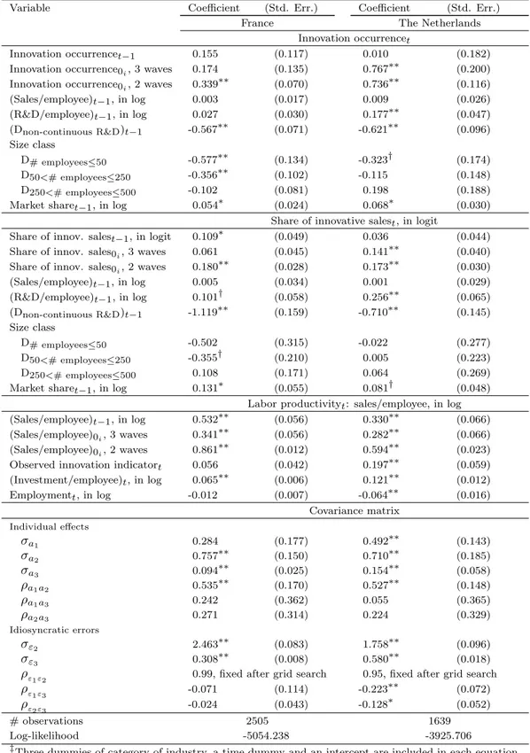
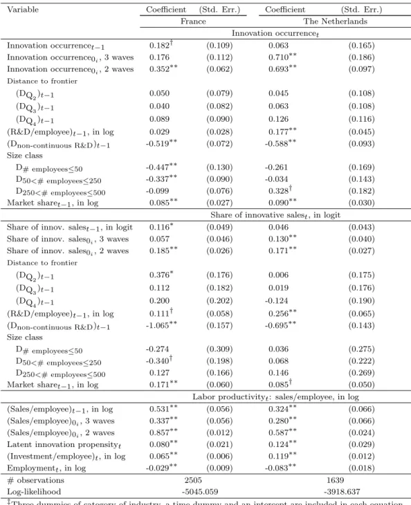
We now turn to the results of the estimation of the models. We shall ﬁrst quickly comment on the general results before discussing particularly the estimated eﬀects of innovation output on productivity and the dynamic interrelations between innovation and productivity. Tables 4 and5 present the estimation results for the model with latent innovation as a predictor of labor productivity, and Tables6 and 7 present the results for the model with observed innovation as a

(18)

predictor of labor productivity.

Table 4: FIML estimates of the model with latent innovation propensity to explain productivity: Unbalanced panel data samples from Dutch and French CIS 2, CIS 3 and CIS 4‡

Variable Coeﬃcient (Std. Err.) Coeﬃcient (Std. Err.)

France The Netherlands

Innovation occurrencet

Innovation occurrencet₋₁ 0.181† (0.103) 0.051 (0.171)

Innovation occurrence0i, 3 waves 0.167 (0.111) 0.696∗∗ (0.189)

Innovation occurrence0i, 2 waves 0.339∗∗ (0.066) 0.721∗∗ (0.112)

(Sales/employee)t−1, in log 0.000 (0.017) 0.010 (0.025) (R&D/employee)t−1, in log 0.025 (0.027) 0.173∗∗ (0.045) (Dnon-continuous R&D)t−1 -0.534∗∗ (0.070) -0.587∗∗ (0.093) Size class D# employees≤50 -0.470∗∗ (0.130) -0.271 (0.170) D50<# employees≤250 -0.335∗∗ (0.092) -0.049 (0.144) D250<# employees≤500 -0.095 (0.077) 0.304† (0.182)

Market sharet₋₁, in log 0.074∗∗ (0.024) 0.077∗∗ (0.029) Share of innovative salest, in logit

Share of innov. salest−1, in logit 0.110∗ (0.050) 0.043 (0.044) Share of innov. sales0i, 3 waves 0.064 (0.046) 0.132∗∗ (0.040)

Share of innov. sales0i, 2 waves 0.185∗∗ (0.027) 0.174∗∗ (0.030)

(Sales/employee)t₋₁, in log 0.002 (0.034) 0.001 (0.029) (R&D/employee)t₋₁, in log 0.105† (0.057) 0.258∗∗ (0.065) (Dnon-continuous R&D)t−1 -1.093∗∗ (0.154) -0.697∗∗ (0.144) Size class D# employees_≤50 -0.349 (0.311) 0.022 (0.276) D50<# employees≤250 -0.361† (0.206) 0.065 (0.222) D250<# employees≤500 0.118 (0.169) 0.156 (0.268)

Market sharet−1, in log 0.152∗∗ (0.055) 0.093∗ (0.047) Labor productivityt: sales/employee, in log (Sales/employee)t₋₁, in log 0.531∗∗ (0.056) 0.319∗∗ (0.066) (Sales/employee)0i, 3 waves 0.336∗∗ (0.056) 0.282∗∗ (0.066)

(Sales/employee)0i, 2 waves 0.856∗∗ (0.012) 0.584∗∗ (0.024)

Latent innovation propensityt 0.074∗∗ (0.020) 0.121∗∗ (0.029) (Investment/employee)t, in log 0.065∗∗ (0.006) 0.119∗∗ (0.012) Employmentt, in log -0.027∗∗ (0.008) -0.082∗∗ (0.018) Covariance matrix Individual eﬀects σa1 0.259† (0.148) 0.470∗∗ (0.138) σa2 0.745∗∗ (0.179) 0.680∗∗ (0.193) σa3 0.096∗∗ (0.025) 0.160∗∗ (0.060) ρa1a2 0.514∗∗ (0.152) 0.540∗∗ (0.145) ρa1a3 -0.090 (0.408) -0.221 (0.336) ρa2a3 0.158 (0.279) 0.064 (0.331) Idiosyncratic errors σε2 2.469∗∗ (0.076) 1.780∗∗ (0.096) σε3 0.313∗∗ (0.009) 0.587∗∗ (0.019)

ρ_ε1ε2 0.99, ﬁxed after grid search 0.95, ﬁxed after grid search

ρ_ε1ε3 -0.206∗∗ (0.071) -0.237∗∗ (0.067)

ρ_ε2ε3 -0.208∗∗ (0.070) -0.229∗∗ (0.061)

# observations 2505 1639

Log-likelihood -5048.917 -3920.898

‡_{Three dummies of category of industry, a time dummy and an intercept are included in each equation.} Signiﬁcance levels : † : 10% ∗ : 5% ∗∗ : 1%

(19)

Table 5: FIML estimates of the model with latent innovation intensity to explain productivity: Unbalanced panel data samples from Dutch and French CIS 2, CIS 3 and CIS 4‡

Innovation occurrencet₋₁ 0.151 (0.098) 0.027 (0.178)

Innovation occurrence0i, 3 waves 0.171† (0.102) 0.738∗∗ (0.194)

(Sales/employee)t−1, in log 0.004 (0.018) 0.009 (0.026) (R&D/employee)t₋₁, in log 0.023 (0.028) 0.173∗∗ (0.047) (Dnon-continuous R&D)t−1 -0.546∗∗ (0.070) -0.607∗∗ (0.095) Size class D# employees_≤50 -0.509∗∗ (0.126) -0.325† (0.175) D50<# employees_≤250 -0.353∗∗ (0.091) -0.101 (0.150) D250<# employees_≤500 -0.111 (0.077) 0.225 (0.187)

Market sharet₋₁, in log 0.069∗∗ (0.024) 0.072∗ (0.030)

Share of innovative salest, in logit

Share of innov. salest₋₁, in logit 0.138∗∗ (0.048) 0.055 (0.043) Share of innov. sales0i, 3 waves 0.044 (0.043) 0.113∗∗ (0.040)

(Sales/employee)t₋₁, in log 0.004 (0.033) -0.001 (0.029) (R&D/employee)t₋₁, in log 0.100† (0.055) 0.261∗∗ (0.062) (Dnon-continuous R&D)t₋₁ -1.018∗∗ (0.154) -0.691∗∗ (0.140) Size class D# employees≤50 -0.187 (0.296) 0.096 (0.271) D50<# employees≤250 -0.366† (0.198) 0.169 (0.219) D250<# employees≤500 0.103 (0.162) 0.323 (0.266)

Labor productivityt: sales/employee, in log (Sales/employee)t₋₁, in log 0.527∗∗ (0.056) 0.320∗∗ (0.066) (Sales/employee)0i, 3 waves 0.337∗∗ (0.056) 0.282∗∗ (0.066)

Latent share of innovative salest 0.043∗∗ (0.010) 0.084∗∗ (0.022) (Investment/employee)t, in log 0.065∗∗ (0.006) 0.120∗∗ (0.012) Employmentt, in log -0.025∗∗ (0.008) -0.070∗∗ (0.017) Covariance matrix Individual eﬀects σa1 0.322∗∗ (0.092) 0.492∗∗ (0.134) σa2 0.673∗∗ (0.190) 0.642∗∗ (0.213) σa3 0.095∗∗ (0.026) 0.158∗∗ (0.060) ρa1a2 0.546∗∗ (0.128) 0.544∗∗ (0.146) ρa1a3 -0.094 (0.315) -0.121 (0.350) ρa2a3 -0.108 (0.302) -0.151 (0.362) Idiosyncratic errors σε2 2.481∗∗ (0.075) 1.791∗∗ (0.098) σε3 0.320∗∗ (0.011) 0.596∗∗ (0.021)

ρ_ε1ε3 -0.298∗∗ (0.077) -0.266∗∗ (0.074)

ρ_ε2ε3 -0.301∗∗ (0.075) -0.288∗∗ (0.073)

Log-likelihood -5045.613 -3922.326

(20)

Table 6: FIML estimates of the model with observed innovation indicator to explain productivity: Unbalanced panel data samples from Dutch and French CIS 2, CIS 3 and CIS 4‡

Innovation occurrencet₋₁ 0.155 (0.117) 0.010 (0.182)

(Sales/employee)t−1, in log 0.003 (0.017) 0.009 (0.026) (R&D/employee)t−1, in log 0.027 (0.030) 0.177∗∗ (0.047) (Dnon-continuous R&D)t−1 -0.567∗∗ (0.071) -0.621∗∗ (0.096) Size class D# employees≤50 -0.577∗∗ (0.134) -0.323† (0.174) D50<# employees_≤250 -0.356∗∗ (0.102) -0.115 (0.148) D250<# employees_≤500 -0.102 (0.081) 0.198 (0.188)

Market sharet₋₁, in log 0.054∗ (0.024) 0.068∗ (0.030)

Share of innov. salest−1, in logit 0.109∗ (0.049) 0.036 (0.044) Share of innov. sales0i, 3 waves 0.061 (0.045) 0.141∗∗ (0.040)

(Sales/employee)t₋₁, in log 0.005 (0.034) 0.001 (0.029) (R&D/employee)t₋₁, in log 0.101† (0.058) 0.256∗∗ (0.065) (Dnon-continuous R&D)t₋₁ -1.119∗∗ (0.159) -0.710∗∗ (0.145) Size class D# employees_≤50 -0.502 (0.315) -0.022 (0.277) D50<# employees≤250 -0.355† (0.210) 0.005 (0.223) D250<# employees≤500 0.108 (0.171) 0.064 (0.269)

Market sharet₋₁, in log 0.131∗ (0.055) 0.081† (0.048)

Observed innovation indicatort 0.056 (0.042) 0.197∗∗ (0.059) (Investment/employee)t, in log 0.065∗∗ (0.006) 0.121∗∗ (0.012) Employmentt, in log -0.012 (0.007) -0.064∗∗ (0.016) Covariance matrix Individual eﬀects σa1 0.284 (0.177) 0.492∗∗ (0.143) σa2 0.757∗∗ (0.150) 0.710∗∗ (0.185) σa3 0.094∗∗ (0.025) 0.154∗∗ (0.058) ρa1a2 0.535∗∗ (0.170) 0.527∗∗ (0.148) ρa1a3 0.242 (0.362) 0.055 (0.365) ρa2a3 0.271 (0.314) 0.224 (0.329) Idiosyncratic errors σε2 2.463∗∗ (0.083) 1.758∗∗ (0.096) σε3 0.308∗∗ (0.008) 0.580∗∗ (0.018)

ρ_ε1ε3 -0.071 (0.114) -0.223∗∗ (0.072)

ρ_ε2ε3 -0.024 (0.043) -0.128∗ (0.052)

Log-likelihood -5054.238 -3925.706

(21)

Table 7: FIML estimates of the model with observed innovation intensity to explain productivity: Unbalanced panel data samples from Dutch and French CIS 2, CIS 3 and CIS 4‡

Innovation occurrencet₋₁ 0.245∗∗ (0.088) 0.014 (0.176)

(Sales/employee)t−1, in log 0.000 (0.016) 0.008 (0.026) (R&D/employee)t₋₁, in log 0.020 (0.026) 0.177∗∗ (0.047) (Dnon-continuous R&D)t−1 -0.433∗∗ (0.063) -0.608∗∗ (0.095) Size class D# employees≤50 -0.514∗∗ (0.115) -0.319† (0.173) D50<# employees_≤250 -0.354∗∗ (0.082) -0.102 (0.148) D250<# employees_≤500 -0.129† (0.069) 0.220 (0.187)

Market sharet−1, in log 0.069∗∗ (0.021) 0.071∗ (0.030)

Share of innov. salest₋₁, in logit 0.139∗∗ (0.041) 0.044 (0.044) Share of innov. sales0i, 3 waves 0.030 (0.036) 0.130∗∗ (0.040)

(Sales/employee)t₋₁, in log 0.002 (0.031) -0.001 (0.029) (R&D/employee)t₋₁, in log 0.076† (0.045) 0.262∗∗ (0.064) (Dnon-continuous R&D)t₋₁ -0.708∗∗ (0.127) -0.690∗∗ (0.144) Size class D# employees≤50 -0.213 (0.258) 0.029 (0.275) D50<# employees≤250 -0.389∗ (0.170) 0.070 (0.221) D250<# employees≤500 0.001 (0.136) 0.178 (0.268)

Observed share of innovative salest 0.107∗∗ (0.009) 0.045∗∗ (0.012) (Investment/employee)t, in log 0.066∗∗ (0.006) 0.120∗∗ (0.012) Employmentt, in log -0.037∗∗ (0.007) -0.071∗∗ (0.017) Covariance matrix Individual eﬀects σa1 0.154 (0.106) 0.494∗∗ (0.132) σa2 0.511∗∗ (0.140) 0.649∗∗ (0.207) σa3 0.133∗∗ (0.019) 0.157∗∗ (0.060) ρa1a2 0.557∗∗ (0.124) 0.550∗∗ (0.139) ρa1a3 0.011 (0.230) -0.002 (0.361) ρa2a3 0.117 (0.195) 0.120 (0.382) Idiosyncratic errors σε2 2.459∗∗ (0.065) 1.795∗∗ (0.098) σε3 0.357∗∗ (0.012) 0.586∗∗ (0.019)

ρ_ε1ε3 -0.570∗∗ (0.042) -0.274∗∗ (0.076)

ρ_ε2ε3 -0.691∗∗ (0.038) -0.259∗∗ (0.069)

Log-likelihood -5021.290 -3923.897

(22)

5.1 The eﬀects of size, market share, R&D, physical capital and the

error terms

It is ﬁrst of all remarkable and comforting to notice that the results are quite consistent and robust across models. Tables 4 to 7 show that larger French manufacturing ﬁrms are more likely to be product innovators while no such evidence is found for Dutch manufacturing.14 _{Size does not seem}

to play, however, a significant role in explaining differences in innovation intensities conditional on being an innovator. For both countries, however, market share plays a positive and significant role not only in the innovation occurrence but also in the share of innovative sales: a 10% increase in market share increases the probability to innovate by 0.2% and the share of innovative sales by 1 to 2%.

In France and The Netherlands, enterprises that undertook R&D activities continuously during the previous two to four years are more likely to be product innovators and attain a larger share of innovative sales. Moreover, past R&D intensity increases both the innovation propensity (and the probability of becoming a product innovator) and intensity of the average Dutch enterprise. The estimates show that a 1% increase in R&D intensity corresponds four years later to an increase in the probability of being a product innovator of about 5%, and to an increase in the share of innovative sales (of product innovators) of about 0.2%.15 _{The estimates are lower for France}

showing that a 1% increase in R&D intensity does not significantly affect the probability to innovate four years later, although it corresponds to an increase in the share of innovative sales of about 0.1% (and significant at the 10% level). Overall our results are also consistent with a lagged impact of R&D on innovation.16

We observe a negative and statistically signiﬁcant correlation, at time t, in both countries and in all speciﬁcations between the idiosyncratic error terms in the innovation and the labor productivity equations. This could correspond to the fact that, in order to innovate, enterprises may need to increase their personnel, which in the short run may lead to a decrease in labor productivity because of adjustment costs and time to learn.17

Note that the estimated elasticities of productivity with respect to labor and physical capital

14_{Since the reference size category consists of ﬁrms with more than 500 employees, the negative signs for the other}

categories indicate a positive size eﬀect.

15_{The marginal eﬀect of a regressor on the probability of the average ﬁrm to become a product innovator is}

obtained in the usual way, (seeGreene,2011, page 689). Furthermore, because of the logit transformation of the share of innovative sales, the R&D elasticity is obtained by multiplying the coeﬃcient of R&D by 1− y2twhere y2t

denotes the share of innovative sales in level (see AppendixC).

16_{To have a better appreciation of the time span between R&D investment and innovation success, we would of}

course need a longer and yearly panel allowing us to estimate a distributed lag model, along the lines for example ofPakes and Griliches(1980) andHall et al.(1986) as regards R&D and patents.

17_{As for the correlation between the two innovation equations, ρ}

ϵ1ϵ2, the log-likelihood values tended to be the

highest for values around 0.95 for The Netherlands and 1 for France, which lead us to ﬁx these values in the estimation.

(23)

shown in Tables4 to 7 are also all statistically signiﬁcant and their orders of magnitude are not unreasonable. In other words, we ﬁnd decreasing elasticities of scale by slightly less than 5% in French manufacturing and slightly more in Dutch manufacturing, and elasticities for physical capital on the low side, especially for France, which could be expected since capital is proxied by investment.

In order to capture enterprises’ unobserved ability to be innovative and productive we account for individual effects in each equation of the model. Likelihood ratio (LR) tests suggest that they have indeed to be taken into account as the specifications assuming their absence in the model are rejected at the 1% significance level.18

5.2 The eﬀects of innovation output on labor productivity

Table 8compares the four sets of estimated elasticities and semi-elasticities of labor productivity with respect to innovation from Tables4 to 7, and presents tests on their equality across the two countries and on whether the models with latent and observed innovation output as a predictor of labor productivity are equally close to the ‘true’ unknown model. All these elasticities are positive and highly statistically significant except in the case of the observed innovation indicator for France. We can make more precisely the following remarks. Firstly, these estimates appear statistically different across countries only in the specification with observed innovation. A product innovator has on average a 20% higher labor productivity than a non-innovator in Dutch manufacturing and a 6% higher labor productivity in French manufacturing. By contrast, in French manufacturing a 1% increase in the share of innovative sales raises labor productivity on average by 0.12%, compared to 0.05% in Dutch manufacturing. Labor productivity is more responsive to increases in product innovation in French than in Dutch manufacturing enterprises.

Secondly, usingVuong’s (1989) LR test for non-nested hypotheses, we conclude that the models, with respectively latent and observed innovation output as a predictor of labor productivity, are equally close to the ‘true’ unknown model. This result contrasts with that ofDuguet(2006) who used a similar test byDavidson and MacKinnon(1981) to conclude that observed innovation is a better predictor of TFP growth than latent innovation. A likely reason for the diﬀerence may be that the two-step estimation procedure used byDuguet(2006) ignores the correlation between the errors in the innovation and productivity equations.

As stressed inMairesse et al. (2005), the important point is that the estimates of innovation output in the productivity equation are signiﬁcant only when the endogeneity of innovation is taken into account, and this is also what appears here. When innovation is treated as exogenous