Algorithms for two-stage flow-shop with a shared machine in stage one and two parallel machines in stage two

UNIVERSITÉ DU QUÉBEC À CHICOUTIMI

MÉMOIRE PRESENTE À

L'UNIVERSITÉ DU QUÉBEC À CHICOUTIMI

COMME EXIGENCE PARTIELLE

DE LA MAÎTRISE EN INFORMATIQUE

OFFERTE A

L'UNIVERSITÉ DU QUÉBEC À CHICOUTIMI

PAR

YANG YANG

ALGORITHMS FOR TWO-STAGE FLOW-SHOP WITH A

SHARED MACHINE IN STAGE ONE AND TWO PARALLEL

ABSTRACT

Scheduling problems may be encountered in many situations in everyday life.

Organizing daily activities and planning a travel itinerary are both examples of small

optimization problems that we try to solve every day without realizing it. However,

when these problems take on larger instances, their resolution becomes a difficult task

to handle due to prohibitive computations that generated.

This dissertation deals with the Two-Stage Flow-shop problem that consists of three

machines and in which we have two sets of jobs. The first set has to be processed, in this

order, by machine M± and then by machine M2. Whereas, the second set of jobs has to be processed, in this order, by machine M± and then by machine M3. As we can see,

machine M1 is a shared machine, and the other two machines are dedicated to each of

the two subsets of jobs.

This problem is known to be strongly NP-Hard. This means there is a little hope that

it can be solved by an exact method in polynomial time. So, special cases, heuristic, and

meta-heuristic methods are well justified for its resolution.

We thus started in this thesis to present special cases of the considered problem

and showed their resolution in polynomial time.

In the approximation front, we solved the considered problem with heuristic and

In the former approach, we designed two heuristic algorithms. The first one is based

on Johnson's rule, whereas the second one is based on Nawez, Enscore, and Ham

algorithm. The experimental study we have undertaken shows that the efficiency and

the quality of the solutions produced by these two heuristic algorithms are high.

In the latter approach, we designed a Particle Swarm Optimization algorithm. This

method is known to be popular because of its easy implementation. However, this

algorithm has many natural shortcomings. We thus combined it with the tabu search

algorithm to compensate the negative effects. The experimental study shows that the

new hybrid algorithm outperforms by far not only the standard Particle Swarm

ACKNOWLEDGEMENTS

First of all, I must give my most sincere thanks to my supervisor Professor Djamal

Rebaïne, for his availability, his involvement and his support throughout his research. I

am particularly grateful that he was attentive to my ideas and comments, and also for

responding too many of my questions. Without this assistance and dynamism, this

research would probably not have been born.

Research work could not be done without financial support. As such, I would like to

thank Professor Djamal Rebaïne again, because he gave me a scholarship to reduce

much of my burden, allowing me to focus on my research.

Secondly, I would also like to thank my parents deeply. They really sacrificed a lot

for me in the past 3 1 years. It is difficult to find the language to express this gratitude. I

can only say that, at present, my greatest wish is to be able to ensure that they live a

happy life forever.

TABLE OF CONTENTS

ABSTRACT I ACKNOWLEDGEMENTS Ill TABLE OF CONTENTS , IV LIST OF TABLES VI LIST OF FIGURES VII Chapter 1 General introduction ....: 8 Chapter 2 Scheduling problems 12 2.1 Introduction 12 2.2 Problem description 15 2.3 Classification of scheduling problems 16 2.4 Flow-shop problem 23 Chapter 3 Concepts of complexity theory 25 3.1 Introduction 25 3.2 Class P and NP 25 3.3 NP-hard and NP-complete problems 26 3.4 Combinatorial optimization problems 28 3.5 Exact algorithms 29 3.5.1 Branch and bound 29 3.5.2 Dynamic programming 30 3.5.3 Reduction methods 30 3.5.4. Constructive methods 3 1 3.6 Approximation approach 31 3.6.1 Heuristic algorithms 3 1 3.6.2 Meta-heuristic algorithms 32 3.7. Solving scheduling problems 35 Chapter 4 Two-stage Flow-shop with a shared machine in stage one and two

parallel machines in stage two 37 4.1 Introduction 37 4.2 Study of special cases 38 4.2.1 First special case: standard two-stage flow-shop 38 4.2.2 Second special case: constant processing times 40 4.2.3 Third special case: Large processing times in Stage 1 48 4.2.4 Fourth special case: Large processing times in Stage 2 53 Chapter 5 Heuristic approach 57

5.1 Introduction 57 5.2 Heuristic algorithms of FSP 57 5.2.1 CDS heuristic algorithm 58 5.2.2 Palmer heuristic algorithm.. 59 5.2.3 RA heuristic algorithm 59 5.2.4 NEH heuristic algorithm 59 5.2.5 Gupta heuristic algorithm 60 5.3 Heuristic design for F 3 | M 1 -> M 2 ; M l -> M3\Cmax 60 5.3.1 A heuristic based on Johnson's rule 6 1 5.3.2 A heuristic based on NEH 65 5.3.3 Experimental study 66 Chapter 6 Meta-heuristic approach 70 6.1 Introduction 70 6.2 Tabu Search (TS) 70 6.2.1 Neighbourhood search 7 1 6.2.2 Principles of Tabu search 73 6.3 Particle Swarm Optimization (PSO) 75 6.3.1 Principles of PSO 75 6.3.2 Process of PSO algorithm 78 6.4 Encoding 79 6.5 Hybridization 82 6.5.1 Features of TS and PSO 82 6.5.2 Design of the hybrid algorithm 84 6.5.3 Experimental study 88 Conclusion 90 References ; 92

LIST OF TABLES

Table 2.1: Processing times of jobs 15 Table 2.2: Processing times of jobs for Example 2.2 23 Table 4 . 1 : Processing times of jobs for Example 4.1 39 Table 5.1: Set of two-machine flow shop problems 58 Table 5.2: Processing times of jobs for Example 5.1 63 Table 5.3: Schedule two subsets by Johnson's rule 63 Table 5.4: Processing times of jobs for Example 5.2 66 Table 5.5.1: Simulation of both heuristics where processing times are in [50,100] . 68 Table 5.5.2: Simulation of both heuristics where processing times are in [20,100] . 68 Table 5.5.3: Simulation of both heuristics where processing times are in [10,100] . 69 Table 5.5.4: Simulation on the heuristic based on Johnson's rule 69 Table 6.1: Processing times of jobs for Example 6.1 72 Table 6.2: Neighbourhood of solution x = (3,4,2,1) 72 Table 6.3: Tabu list after the first iteration 73 Table 6.4: Tabu list after the second iteration 73 Table 6.5: Position of the particle and the corresponding ROV value 80 Table 6.6: After SWAP operations, the particle component position is adjusted 82 Table 6.7: Characteristics of TS and PSO approaches 83 Table 6.8: Initial tabu list and swarm 85 Table 6.9: The tabu list and swarm after first iteration 85 Table 6.10: The tabu list and swarm after second iteration 86 Table 6.11: The tabu list and swarm (Unified Pardon Rule) 86 Table 6.12: The tabu list and swarm (Prioritized Pardon Rule) 86 Table 6.13.1: Simulation of hybrid PSO where processing times are in [50,100] 89 Table 6.13.2: Simulation of hybrid PSO where Processing times are in [20,100] 89 Table 6.13.3: Simulation of hybrid PSO where Processing times are in [10,100] 89

LIST OF FIGURES

Figure 1.1: The model studied 10 Figure 2.1 CIM and a production control system 13 Figure 2.2 Two Gantt charts for Example 2.1 16 Figure 2.3: Gantt chart for order A->B->C->D 24 Figure 2.4: Gantt chart for order B->D->C->A 24 Figure 3.1: Relationship between NP, P, and NPC classes. 27 Figure 4.1: Two-stage flow-shop with one shared machine in stage one and two

parallel machines in stage two 38 Figure 4.2: Divide the problem into two standard two-stage flow-shop problems....39 Figure 4.3: Gantt chart for the case p1 = p2 = V 41

Figure 4.4: Size o f /x larger than that of J2 44

Figure 4.5: Size of J2 larger than that ofj1 45

Figure 4.6: [ y ] < nx 47

Figure 4.7: I —I >n± 47

L AC J

Figure 4.8: Crossed scheduling for the jobs of/x and/2 50 Figure 4.9:/! is processed before J2 50 Figure 4.10: No change on the makespan after inserting j o b / 54 Figure 4.11: One job of another subset between two jobs of either J± or J2 55 Figure 5.1: Minimal value of two functions 62 Figure 6.1: Model of the swarm of RSO 76 Figure 6.2: Updating the particle 77

Chapter 1

General introduction

The theory of scheduling is one well-established discipline of combinatorial

optimization field. A scheduling problem involves organizing, over time, the realization

of a set of jobs over a set of resources, usually named as machines.

A job ji is composed of n different operations { O Q , 0i2f..., 0 jn} , and every operation

requires a period of time t y . The machine is a kind of technique or human resource to

be used to carry out jobs, and it is available in limited proportions and capacities.

The evaluation of a scheduling solution is compared to one or more goals of

performance that satisfy certain conditions of treatment.

The popularity of scheduling theory stems from the fact that a multitude of

situations encountered in practice within companies and organizations that can be

reduced to the problems of scheduling. For example, machines may represent

processors and jobs, nurses and patients, workers and products, etc.

Among the scheduling problems that have been studied in the literature, the

problem of serial workshops (Flow-shop Scheduling Problem, FSP) is one of the first that

was studied in the early fifties. Johnson, in 1954, was the first to examine and design an

efficient solution for the Flow-shop with two machines [Johnson, 1954]. Since then,

the theory and what actually happens in the centres of production. We may mention

the following constraints that the theory of scheduling has not considered until recently.

1. The latency of the work corresponding to the different time needed between

the end of an operation and the beginning of the next operation in the same job.

For example, the cooling time before their next job manipulation. These times,

in some cases to a significant degree, must not be ignored, but in others cases,

we could incorporate latency into the processing time of an operation to reduce

the complexity of the problem. However, the correctness of the solution will be

only slightly influenced or not at all affected.

2. Resources constraints corresponding to the situation where jobs cannot be

processed unless sufficient (human or else) resources are available.

Research in scheduling can be divided into two parts: modelling and algorithm

design. The modelling part is about designing appropriate mathematical models to

capture the complexity of real problems, whereas the algorithm design part is about the

design of analysis of algorithms, the convergence algorithms and the optimization

quality.

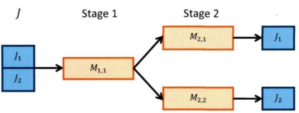
In this dissertation, we study the model of flow-shop with two stages as Figure 1.1.

The criterion we seek to minimize the overall completion time of the jobs, known as the

makespan. This problem may be defined as follows.

We are given a set J of n independent jobs partitioned in two disjoint subsets that

have to be scheduled on a two-stage flow-shop: the first stage contains one machine

processed first by the machine of the first stage, and then by on machine of the second

stage. The second subset is processed by the machine of the first stage, the by the other

machine of the second stage. We assume that all of the jobs are available at time 0 and

have exactly two operations executed on two different machines; the transportation

time and latency are included in the processing time of operation; pre-emption is not

allowed and the machines in the model are always available and can process only one

job at one time [Chikhi, Boudhar, and Soukhal, 2011]. This problem is strongly NP-hard

[Tuong Soukhal and Miscopein, 2009].

Set N of Jobs each of which has two operations. Two subsets of job Jx a n d /2/ / i u/ 2 = 1 •

Subset/j must be executed by machine 1 and then by machine 2,1. Subset]2 must be executed by machine 1 and then by machine 2,2.

The order of the jobs is the same at each stage.

Figure 1.1: The model studied

Our study is three folds. First, we seek polynomial time algorithms to solve this

model in some special cases, in our case the processing times are special pattern. The

second goal is to solve the general model by two meta-heuristic algorithms. The third

goal is to improve the original meta-heuristic and make it more efficient for our model.

This thesis is divided into six chapters. Besides this present chapter, Chapter 2

introduces the different models encountered in the theory of scheduling. Chapter 3 is

devoted to the basic concepts used in the complexity theory, along with the different

methods used when confronted with an NP-difficult problem. Chapter 4 first proposes a

formulation of the problem we are considering, and then presents several special cases

along with their solving algorithms and proofs of their optimality. Chapter 5 is devoted

to the study of the heuristic approach. In this chapter, we proposed two new algorithms

along with an experimental study to discuss their performance. Chapter 6 is about the

meta-heuristic approach. In this chapter, we first proposed two meta-heuristic

algorithms: one is based on the tabu search approach, and the second is based on the

particle swarm optimization approach. After studying their respective performance

through an experimental simulation, we proposed a third approach which is a

hybridisation of the two approaches. Again an experimental study is performed to see

Chapter 2

Scheduling problems

2.1 Introduction

With the development of science and technology, the scale of production has

become increasingly important, and the process of production has also become more

and more complicated, and market competition is getting increasingly fierce. In this

environment, organizations have to face increasingly greater numbers of problems, such

as the control of production process in response to changing production planning, and

also how to maximize their interests or efficiencies.

As a solution to these problems, [Harrington, 1974] introduced the concept of CIM

(computer integrated manufacturing), as pictured by Figure 2.1. CIM is a manufacturing

approach in which computers are used to control the entire production process [Serope

and Steven, 2006]. In a CIM system, functional areas such as design, analysis, planning,

purchasing, cost accounting, inventory control and distribution are all linked through the

computer with factory floor functions such as material handling and management,

thereby allowing monitoring of all of the operations.

The production plan is an important component of CIM as it plays a substantial role

in the entire operation of an enterprise. The task of the production plan is to maximize

the benefits of the targeted companies. The development of a production plan is

generally considered as a static situation. The production plan is executed by the scheduling system. ReqpestfertsiimaiiS Proposais 1 * 7 Oesigû, Chatty peftamanoe i / methods,

I /

What and wheft?

t

Figure 2.1 CM and a production control system [Toni and Tonchia, 1998]

Production scheduling plans the production process as a decisive advantage, which

is t h e core of t h e production plan. An efficient scheduling m e t h o d is a key t o improve t h e efficiency of production. Improvements in production scheduling n o w allow us t o pay more attention t o improving t h e efficiency o f production and resource use. Production scheduling is based on t h e production plan and depends on market demands and conditions and technical equipment. The task of production scheduling is t o plan and organize t h e production process. Its main factors are as follows:

(1) The n u m b e r of products. (2) Production Line.

(4) The production constraints.

In the field of theoretical research, production planning and production scheduling

are referred to as scheduling problems. The difference between them is that the

production planning principally considers the long-term plan while neglecting or

simplifying production constraints. In contrast, production scheduling considers the plan

in the short term; its main purpose is to organize the production and distribute

resources over time. So, it must take into account a variety of constraints in the real

production environment. Therefore, production scheduling is the process of achieving

the production plan.

A scheduling problem involves the organization, overtime, of the realization of a set

of tasks based on the resource availability.

Production management may differ for different optimization objectives, such as

strategy optimization or model optimization of a scheduling problem. Each production

environment is almost unique because of the dynamics of the production environment

and the diversity of the knowledge production, which makes it difficult to find a

corresponding method for all situations. Scheduling problems are usually of

optimization nature and are part of the combinatorial optimization class (for more

details see Section 3.4). It is worth to mention that the vast majority of scheduling

problems turn out to be NP-complete (see the definition in Chapter 3). When a problem

is shown to be an NP-complete problem, this means that there is a little hope to find an

exact algorithm to solve it within a reasonable time. The use of approximation approach

or the design of well solvable cases is therefore justified.

2.2 Problem description

Scheduling problems are described basically by two sets:

/ = {JiJ2> — Jn) of n jobs that will be executed in the system.

- M = {Mlt M2,..., Mm} of m machines present in the system to process set J. A scheduling problem involves assigning the set M to complete all jobs o f / with

some constraints/Scheduling has two constraints: occupation constraints and order

constraints. Occupation constraints indicate that each job is executed by at most one

machine at the same time and that each machine can process at most one job at the

same time; order constraints indicate that each job must be executed in a certain order.

All scheduling solutions can be represented by a diagram called the Gantt chart.

This is a type of bar charts, developed by Gantt [Gantt, 1910]. These diagrams help to

visualize a solution. Gantt charts illustrate the starting and finishing dates of the

terminal elements and summary elements of a project. Terminal elements and summary

elements comprise the work breakdown structure of the project. The chart has two

perpendicular axes; the horizontal axis represents the time units, while the vertical axis

represents the machines that are in the centre.

Example 2.1: Let J = {JlfJ2/ ••• ,]v), with n = 3, and M — {Mlf M2,..., Mm}, with m = 2. Table 2.1 shows the processing time for each job.

Mi M2

h

h

h

Figure 2.2 shows the Gantt chart associated with the scheduling solution. From this

diagram, we can determine the value of the criterion we considered. This diagram may

help to determine the strength or the weakness of this solution.

Machines

M

(a) A machine-oriented Gantt chart for example 2-1

i Machines

A

h

h

M

| M

M

|

(b) A job-oriented Gantt chart for example 2-1 Figure 2.2 Two Gantt charts for Example 2.1

2.3 Classification of scheduling problems

The variety of scheduling problems that arise in practice leads to a notation that

allows us to classify them. This notation was first proposed by Graham et al. (1979) and

expanded later by several authors to include other new scheduling problems.

This notation comprises three fields and is of the form a\P\y . The first field a

represents the environment of the machines; the second field (5 describes the

characteristics of the jobs and the resources that are utilized, and the third field y

represents the criterion (or the set of criteria) we are optimizing.

Let us now go into details. Field a consists of two parameters ax and a2 :

a± G { 0 , P, Q, R, PMPM, QMPM, G,X, 0, J F] and ct2 are equal to positive integer

1. If <*! G { 0 , P, Q; R, PMPM, QMPM}: any job comprises one single operation.

2. If <*! = 0 : we have one single machine to process the set of jobs. The processing

times Pij are reduced to pj.

3. If c*! G {P, Q, R}, then we have a set of m machines (m > 1) operating in parallel,

that is to say each job can be processed by one of the machines M1 ;. . . , Mm. Usually

we distinguish between three models as below according to the speed of the

machines:

a. If a± = P, then the machines are identical, and thus the speed is the same for

the machines. The processing time pjj of job Jj on Mj are reduced to Pi for all

machines Mj.

b. b. If cti = Q, then the machines have related speeds, and we say that the

machines are uniform. Indeed, within this model, the processing times become

as Pij = Pi/Sj where Sj is the speed of machine Mj.

c. Finally, if ax = R, then there is no relationship between their speeds, and the

machine are said to be unrelated. In this case, the processing times depend on

the machine in which the jobs are processed. So the notation p^ denote the

4. If a ! = PMPM or a± = QMPM, then we have multi-purpose machine model with

identical and uniform speeds, respectively.

5. If ax E {G,X, 0, J F}, then we have a multi-operational model known as the general

shop. This means that the jobs comprise several operations. We indicate the

general shop by setting ax = G. Job shops, flow-shops, open shops, and mixed

shops are special cases of the general shop. The differences are based on the nature

of the job routing.

a. The job shop is indicated by at = J. In this case, an associated route through

the machine is associated with each job.

b. The Flow-shop is indicated by ax = F. In this case, the route though the

machine is the same for the whole set of jobs; by convention each job start from

machine 1, and then machine 1, and so on, until reaching machine m. If addition,

if the same order of processing is kept through all the machines, then we have a

restricted model (which exists in its own right) known as the permutation flow

shop. There are some situations where this model is dominant over the set of all

the solution of a flow shop model.

c. The open shop is indicated by a± = 0. The route of processing of the jobs, in

this case, is not known in advance, but is part of the solution.

d. The mixed shop indicated by at = X is a combination of a flow shop and an

open shop (the combination of a job shop and an open shop is known as the

Parameter cx2 denotes the number of machines utilized if ct2 = k. However, this value is

fixed in advance. Thus/it is part of the input of the problem. If the number of machines

is arbitrary, we set oc2 = 0 .

The second field p describes the characteristics of the jobs and resources utilized. It

comprises eight parameters J31j32j33j34p5fi6j37ps.

• pxe {0,pmtn} indicates whether pre-emption is permitted or not.

• P2 e{0,res} indicates whether resources considerations are taken into account. The

presence of res means that additional resources other than machines (such as

manpower) are needed for the processing of jobs. In case parameter res is not

empty, then it is further divided into three fields "res AoS " denoting respectively

the number of resources, the total amount of available resources per time unit, and

the maximum resource requirements of operations. Note that a dot "." for each of

these parameters indicates that the corresponding variable can take any integer

value, whereas a positive integer indicates that the corresponding variable is fixed.

Moreover, researchers in this area distinguish between renewable and

non-renewable resources.

• J33 E { 0 , prec} indicates whether precedence relations exists between jobs.

Sometimes, we only consider special graphs. In this case, we have to specify the

nature of this graph. Usually we consider tree (denoted by tree), chains (denoted by

chains), series-parallel graphs (denoted by sp-graph).

• /?4 e{0,rj} indicates whether release dates are associated with jobs. Otherwise,

• jB5 G{0,pij = 1, p. = p, px<ptj <p2} indicates special values that can be taken by

the processing times of the jobs. Other values are also possible. The case of 0

indicates that the processing times are arbitrary.

• J36 e{0,df} indicates whether deadlines for the jobs are considered.

• /?7 e{0,ni <k) indicates the maximal number of operations of jobs in the case of a

job shop model.

• /?8 G { 0 , nowait} indicates in the case of shop models whether the processing of the

jobs is done in a no-wait manner. This means that once a job is completed in a

machine, it should immediately, without any waiting time, start its processing in the

following machine.

The third field y represents the criterion we are optimizing. The quality of a

schedule is evaluated to a given criterion (or to a set of given criteria if we are in a

multi-objective environment). In scheduling theory, several criteria are considered in the

literature to build a solution; Mellor [Mellor, 1966] enumerated 26 different criteria.

Associated with each job Jf is a function y^ that depends on the completion time Ci of that

job. Basically two type of objective function are considered in the literature:

1. Bottleneck objective function fW2^ = m a xb^ ,I / ( C - ) .

2. Sum of objective functions

Even though Mellor [Mellor, 1966] has enumerated more than 27 criteria (some of

them are equivalent between each other), the most common criteria utilized in the

literature in building a scheduling solution are as follows:

a. The overall completion time (known as the makespan): C =maxC,.

1<7<«

b. The mean finish time:

7 = 1

n

c. The maxim lateness: L^ = m a x f e ~

i\

d. The number of tardy jobs: 2mdUi where Uj = l i f Ci < di, 0 otherwise.

7 = 1

e. The total tardiness: ^maxjO^C, -dt\

7 = 1

Let us first mention that when deadline are specified, then in some cases there is no need

to minimize an objective function. The only problem we need to solve is to find a feasible

solution. If it is the case, then the field y =

Let us also mention that we usually differentiate between two types of criteria:

regular and non-regular.

Definition 2.1: A criterion is regular if it is non-increasing with respect to the

completion times of the job.

Most of the research in scheduling theory has been done under the assumption that

criteria considered are regular. However, a few papers appeared in the literature in

which non regular criteria are also studied (for more details see for e.g. [Raghavachari,

1988].

Definition 2.2: A schedule is called semi active when machines never idle if they can

Theorem [Brucker, 1995] Semi-active schedules are dominant with respect to regular

criteria.

To conclude a scheduling problem is fully described by the above notation. As an

illustration, the following problems denote:

1. l\prec,pmtn\ C^ : scheduling problem with a single machine, the jobs are

related by a general precedence graph, and pre-emption is allowed. The criterion

to minimize is the makespan.

2. Pm \treer)pi = l , r . \L1SBgi: scheduling problem with m (fixed) identical machines

operating in parallel, the precedence constraints form a tree, the processing

times are unitary, each job is associated with a release date, and deadline which

is stated in the criterion Zmax to be minimized.

3. Fm\no — wait\^jcoiCi\ flow shop problem with no-wait in process. The

criterion to minimize is the mean weighted finish time.

Let us recapitulate. The goal is to build a schedule that generates an optimal (or a

near optimal) solution with respect to a given criterion (or several criteria if we are in a

multi-objective environment; however this is not the case in this thesis). We will assume

throughout this dissertation that all the parameters are known in advance.

Definition 2.3: A solution is feasible if a machine does not process more than one job at

a time, and a job is not processed by more than one machine at a time. In addition,

depending on the problem, a number of specific characteristics may be requested to be

satisfied.

Definition 2.4: We say that a schedule is optimal if it minimizes a given criterion.

2.4 Flow-shop problem

In this dissertation, FSP is the problem we will be focussing on. The Flow-shop

scheduling problem (FSP) can be described as follows:

A set of n jobs is to be processed by Stage 1, Stage 2, and so on until reaching Stage

m, in that order. Each centre may have more than one machine operating in parallel.

The processing time ttj ( i = 1,2, ...,n;y = 1,2, ...,m)of job i in centre y is given. For the FSP, we usually make the following assumptions:

(1) Each machine can only process one job, at the same time.

(2) A job cannot be processed by two machines at the same time.

The preparation time is included in the processing time, and has nothing to do with the

order.

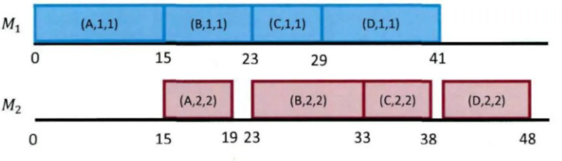
Example 2.2: Let A, B, C, D be 4 jobs, where every job includes two operations 0lf 02 and the processing times are shown in Table 2.2.

Jobs

A

B

C

15

8

6

t

4

10

5

Table 2.2: Processing times of jobs for Example 2.2

Here, tx is the processing time of operation 0x and t2 is the processing time of

operation 02- O n e machine, Mj., is in operation 0x and another machine M2 is in operation 02. In the above scheduling problem, we use three variables (i,j,k) to express that the operation y of job i is executed by machine k. If the jobs are executed

with order A, B, C, and D, then the Gantt chart that expresses it, as it is pictured by Figure 2.3. 1 (A,l,l) 0 2 15 (B,l,l) (A,2,2) (C,l,l) 23 (B, 29 2,2) D,l,l) (C,2,2) 4] (D,2,2) Af, 0 15 19 23 33 38 48

Figure 2.3: Gantt chart for order A->B->C-^D

In Figure 2.3, the boxes represent the operations while the length of the box indicates

the processing time ttjk of the operation (i,j,k).

In a Gantt chart, a feasible schedule should ensure the order of jobs and that no

overlap occurs between boxes. For this example, if we change the job order to B, D, C,

and A, and the corresponding Gantt chart is shown in Figure 2.4.

41

Af,

0 8 18 20

Figure 2.4: Gantt chart for order

27 _{32 41} 45

The makespan of the first schedule is 48, while the makespan of the second schedule is

45. So, we may conclude that the second solution is better than the first one.

Chapter 3

Concepts of complexity theory

3.1 Introduction

Complexity theory is used to measure the degree of difficulty to solve given problem.

Intuitively, if longer computing time is needed to solve a problem, we could say this

problem is harder, otherwise, we say the problem is easier. An important source of

information about this theory is the book of [Garey and Johnson, 1979].

3.2 Class P and NP

Polynomial time is the central concept in computational complexity. This is the

criterion that determines whether an algorithm finds a solution efficiently. Let us recall

that a polynomial time algorithm is an algorithm whose running time is bounded above

by a polynomial expression of the size of the input of the considered problem.

Definition 3.1: Class P is the class of problems for which there exists a polynomial time

algorithm that solve them.

However, there exist problems for which we do not know whether there exist

polynomial time algorithms for their resolution. In order to proceed we need first to

introduce another class named the NP class.

Intuitively, NP class represents the set of all decision problems (see the definition

were given a candidate answer, we are able to verify that whether it is the right answer

of our question in polynomial time. From this definition, it is easy to observe that class P

is a subset of class NP.

3.3 NP-hard and NP-complete problems

Besides class P, there is also another subclass of NP class called NP-complete (NPC

for short) class. This class contains the hardest problems of NP in the following sense.

Definition 3.2: NP-Complete class is a class that is composed of problems that:

Belong to class NP.

If only one problem of that class can be solved in polynomial time, then every

problem in that class can also be solved in polynomial time.

The central notion behind NP-completeness is the concept decision problems and

the concept of polynomial reduction (transformation).

Definition 3.3: A decision problem is a problem for which the solution is a yes or a no

answer.

Definition 3.4: A decision problem L is said to be reducible to another decision problem

K if we can transform an instance of problem L into a instance of problem K in such a

way there is yes-answer to problem L if, and only if, there is a yes-answer problem K.

In order to prove the NP-completeness of a problem L, from above/we proceed as

follows.

1. First, show that the decision version of the considered problem is class NP.

2. Find a known NP-complete problem K and a construct a polynomial reduction

from L to K such that there is a yes answer to L if, and only if, there is yes answer

to problem K.

In other word, we have to prove that problem L is a special case of problem K. Let us

also observe that proving that a problem is NP-hard means only that there exists at least

one instance of that problem which is difficult to solve. In other words, there can be

instances of that problem which can be solved efficiently.

[Cook, 1971] was the first to prove the existence of such a problem known as the

satisfiability problem. Shortly after this important result, 21 other problems were

proved to be NP-complete by [Karp, 1972]. Nowadays, thousands of problems have

been proved to be NP-complete. In fact, as cited in [Graham et al., 1979] the vast

majority of combinatorial optimization problems (the definition follows shortly) are

NP-complete.

Figure 3.1 resumes the relationship between NP, P, and NP-complete classes.

The most important open question in the complexity theory is whether P = NP, that

is to say whether all problems in NP can be solved in polynomial time. This widely

believed not to be the case.

Before closing this section, let us make the following observations. First, when we

talk about optimization problem problems, we prefer to use the term NP-hard problem

when its corresponding decision version is NP-complete. Second, when we talk about

the encoding of an input, we mean the binary encoding. However, even if it is not used

in practice, one could also use the unary encoding. Within that respect, in the

complexity theory, the degree of hardness of a problem is further refined.

Definition 3.5: A problem is complete in the strong sense if it still remains

NP-complete even if the input is encoded in unary.

Definition 3.5: A problem is NP-complete in the weak sense if it can be solved in

polynomial time within the unary encoding. This type of algorithm is called

pseudo-polynomial time.

3.4 Combinatorial optimization problems

Combinatorial optimization is a topic of operations research that consists of finding

an optimal solution from a finite set of solution, which constitutes the search (solution)

space. These kinds of problems are involved in many areas such as: information

technology, timetabling, production scheduling, graph theory, transportation,

bioinformatics, and so on. Let us observe that, even though the solution space is finite,

solution space is huge to enumerate in a reasonable time even with the fastest

computer.

Most of combinatorial optimization problems are NP-Complete problem as are

scheduling problems. However, for small instances they can still be solved efficiently. In

what follows, we describe some resolution techniques that are used to solve scheduling

problems.

3.5 Exact algorithms

In what follows we will be discussing a number of approaches used to solve

combinatorial optimization problems.

3.5.1 Branch and bound

A branch and bound algorithm consists of breaking up the target problem into successively smaller sub-problems, computing bounds on the objective function associated with each sub-problem, and using them to discard certain of these sub^ problems from further consideration. The procedure ends up when each sub-problem has either produced a feasible solution or been shown to contain no better solution than the one already in hand. The best solution found at the end of the procedure is the global optimum. Applying a branch-and-bound algorithm requires specifying the several ingredients (lower bounds, dominance rules, search strategies, etc). It is worth mentioning that the effectiveness of branch and bound algorithms relies not only on the tightness of these ingredients but also on the running time to compute them. For more details on this technique see for e.g. [Balas and Toth, 1985].

3.5.2 Dynamic programming

The method of dynamic programming is an approach, which starts by establishing a

recursion to link the optimal solution of the whole problem under consideration to

those of its sub-problems. Then by carefully implementing this recursion though the use

of a table, we avoid solving sub-problems several times. When the number of different

sub-problems is polynomially bounded, the dynamic programming approach generates

efficient solutions. For more details on this approach, see for e.g. [Dasgupta etal., 2007].

3.5.3 Reduction methods

This method consists of reducing the problem under study into another problem for

which a method of resolution is already known. The most used one are the following.

However, one could use other problems to reduce the original problem into them. For

more details on this approach, see for e.g. [Levitin, 2003].

1. Graph theory: this approach consists of translating the problem into an

equivalent problem of graph theory, such as travelling salesman problem, graph

coloration, shortest path, linear assignment, etc.

2. Mathematical programming: this approach consists of formulating the problem

into a mathematical program by introducing suitable decision variables and an

objective function. We usually try either the linear programming formulations

with or without integer variables. The reason is that for those formulations,

there exist several resolution methods, and certain of them are quite efficient

such as the simplex methods. On the other hand, from the computational point

of view, when we succeed to derive a linear formulation, this means that the

corresponding problem can be classified as an easy problem.

3.5.4. Constructive methods

This approach uses some properties related to the problem under study to generate

simple rules that may lead to the solution of the considered problem. We may mention

Johnson rule that solves to optimality the two-machine problem with respect to the

overall completion time criterion.

3.6 Approximation approach

Approximation algorithms are methods that find near optimal solutions. They are

often used to solve NP-hard problems since it is unlikely that these problems can be

solved exactly by efficient methods.

We usually distinguish between two types of approximation techniques: the

heuristic approach and the meta-heuristic approach. In the former, only one solution is

generated, whereas in the second approach, several solutions may be generated

iteratively.

3.6.1 Heuristic algorithms

Heuristic algorithms usually start with an empty solution. According to some

predefined rules for the problem under study, the algorithm expands the partial

solution at each iteration until getting into the complete solution. Greedy methods and

list scheduling fall into this category of algorithms. The strength of these algorithms is

optimal. Even though, for some problems this way of proceeding may lead to optimal

solutions as it is the case for Johnson rule in the-two machine flow shop problem for the

makespan criterion or the Shortest Processing Time rule in the single machine problem

for the mean finish time criterion.

Heuristic algorithms may produce results by themselves, or they may be used in

conjunction with optimization algorithms to improve their efficiency (e.g., they may be

used to generate good seed values).

Let us mention an important feature of heuristic algorithms. They lend themselves

to a mathematical analysis. This analysis measures the distance that separates the

optimum solution (that we do not know) to the value of the solution produced by this

algorithm. Thus evaluation may be undertaken in the worst case or in the probabilistic

case. In the former, the goal if to find an upper bound on this distance; for more details,

see for e.g. [Fisher, 1982]. In the latter, we measure this distance by means of average

and standard deviation; for more details, see for e.g. [Rinnooy Kan, 1986].

3.6.2 Meta-heuristic algorithms

A meta-heuristic algorithm, also called ameliorative methods, is a method that

solves a problem (usually of optimization nature) by iteratively trying to improve a

candidate solution over the space of feasible solutions with regard to a given measure

of quality, without guaranteeing the optimal solution. Let us point out that the main

difference between meta-heuristic algorithms and heuristic algorithms is that the

former produce several solutions, whereas the latter generate one single solution.

Popular meta-heuristic algorithms for combinatorial optimization problems include

simulated annealing [Kirkpatrick, Gelatt, and Vecchi, 1983], genetic algorithms [Holland,

1975], ant colony optimization [Dorigo, 1992], scatter search [Glover, 1977], tabu search

[Glover, 1986], and particle swarm optimization [Kennedy and Eberhart, 1995]. Tabu

search algorithm and Particle swarm optimization algorithm are discussed in details in

Chapter 6. For the sake of completeness, we present briefly in the following some of the

above cited meta-heuristic algorithms. For a general view on these techniques, see for

e.g. [Fatos and Ajith, 2008].

1. Hill climbing (steepest descent) technique: This method is an iterative search

procedure that, starting from an initial feasible solution, progressively improves it by

applying a series of local modifications. At each iteration of the algorithm, the algorithm

moves to a better feasible solution. The search terminates when no more improvement

is possible. The major drawback of this approach is that, since it is somehow greedy, it

ends up in a local optimum frequently of low quality. Meta-heuristic algorithms (such as

the ones that follow) extend steepest descent methods by allowing the search beyond

the first local optimum. An immediate improvement of this technique is to repeat the

hill climbing technique from several different initial feasible solutions.

2. Simulated annealing algorithm: Annealing is t h e process of slowly cooling a

physical system in order t o obtain states w i t h globally minimum energy. By simulating

such a process, near globally-minimum-cost solutions can be generated in a efficient

way. The corresponding algorithm (see for e.g. [Kirpatrick, Gelatt, and Vecchi, 1983])

are worse than the current solution. The probability of such acceptance decreases over

time. In order to apply the Simulated Annealing method to a specific problem, the

following parameters must be specified: the search space, the objective function, the

neighborhood of solution S, the initial temperature, the cooling factor, and the stopping

criteria. The choice of these parameters has a significant impact on the efficiency of the

method.

3. Genetic algorithms: Genetic algorithm (GA), introduced by [Holland, 1975] is a

method that uses techniques inspired by natural evolution, such as inheritance,

mutation, selection, and crossover. Indeed, once the fitness function is defined, which is

associated to the objective function, the genetic algorithm consists of improving an

initial set of solutions, generated usually at random, through the use of application of

the mutation, crossover, and selection operators. Crossover operator consists in

generating new solutions by combining candidate solutions, whereas the mutation

operator generates a solution by slightly changing a candidate solution. Basically, a

genetic algorithm starts from an initial set candidate solutions, say P, and repeats the

following steps until some stopping criterion is reached:

a. Generate a set of new solutions, say Q, from the set of solutions that can be

obtained from P through the use of crossover and mutation operators.

b. Choose a subset TŒQUP according to the selection rule, and set P = T.

For more details, see for e.g. [Yagiura and Ibaraki, 2001].

3.7. Solving scheduling problems

We present in this section the methodology to follow in order to solve a scheduling problem.

Indeed, the first question to ask, when confronted to a scheduling problem, is whether the

problem is NP-hard or not. The only way to state that a problem is easy to solve is to exhibit a

polynomial solution. If the problem has already been shown to be in the class P, then we usually

try to design other solutions with a better time complexity than the existing solution. If, on the

other hand, the problem under study is shown to be NP-hard, then several approaches can be

tried.

1. We could tight up the NP-hardness by showing the NP-hardness in the strong

sense, or by exhibiting a pseudo-polynomial time algorithm.

2. We could also study to what extent the problem can be solved efficiently by

designing polynomial solutions to special cases. What we mean by that is we

relax some constraints of the problem and see whether the problem is well

solvable or it is still NP-hard. In scheduling problem, we usually consider the

cases where the processing times are restricted to some particular values, we

assume that preemption is permitted; the precedence graphs are of special

types if precedence relations exist between jobs, etc.

3. Design exact algorithms (branch and bound, dynamic programming,

mathematical formulation, etc.) and try to solve larger input of the problem

through the design of ad hoc properties (tight lower bound bounds, strong

dominance relations, etc.).

4. The approximation approach by designing either heuristic algorithms or a

a. If we have chosen the heuristic approach, then the goal here is generally

to undertake a worst-case analysis and get a better ratio by measuring the

distance between the optimal value and the value produced by the

heuristic algorithm. A simulation is also performed to measure the

effectiveness of the proposed solution.

b. If we have preferred the meta-heuristic approach, then in this case we try

to design efficient solutions that solve large instances. In the recent years,

many papers appeared in the literature combined two or more

met-heuristic algorithms. This approach seems to be promising as the results

they produce are by far much better.

Chapter 4

Two-stage Flow-shop with a shared machine in

stage one and two parallel machines in stage two

4.1 Introduction

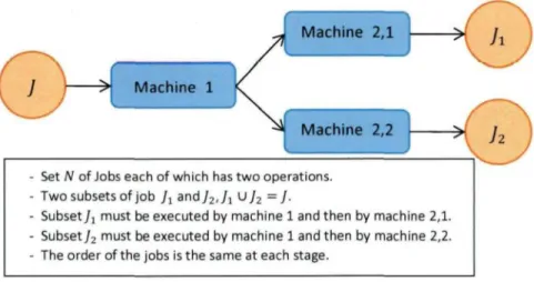
In this dissertation, we study one kind of FSP, named Two-Stage Flow-shop with one

shared machine in stage 1 and two parallel machines in stage two. It is denoted

by F3\M1 -» M2,M\ -» M3\Cmax. This problem may be described as follows.

We are given a set of n independent jobs to be distributed in two disjoint subsets

and scheduled on a two-Stage Flow-shop. The first Stage contains one machine and the

second one contains two machines operating in parallel. We assume that all jobs are

available at time 0 and have exactly two operations to be executed by the two stages.

Furthermore, the jobs in the first subset must be executed on the machine of stage one,

and on machine of stage two, whereas, the jobs of the second subset must be processed

by the machine of stage one, and the other machine of stage two (as illustrated by

Figure 4.1).

The processing times of each job in each Stage are not equal to 0; the transport

time between different Stages are included in the processing time; the three machines

are always available and can process only one job at a time, and one job can be

executed by only one machine at a time. The goal is to minimize the makespan of the

Stage 1

Stage 2

h

h

M2,1

'2,2

Figure 4.1: Two-stage flow-shop with one shared machine in stage one and two parallel machines in Stage two

Even though a problem is NP-hard, there might still are special instances for which

this problem may be solvable in polynomial time. In this section, Then, several special

cases for which the corresponding problem is well solved are discussed.

4.2 Study of special cases

This section is devoted to the presentation of special cases that are solvable in

polynomial time.

4.2.1 First special case: standard two-stage flow-shop

We consider the following two cases:]x = 0 or/2 = 0. This means that Stage 2 is

reduced to one machine. In this case, this problem corresponds to the standard

flow-shop, as illustrated by Figure 4.2.

Figure 4.2: Divide the problem into two standard Two-stage flow-shop problems

This problem can then be solved by the Johnson's rule. Johnson's rule may be

resumed as follows: If min{pii l, p7- 2] — m^n{Pi,2' Vj,\\>tnen job i precedes job ; .

We can use this rule to construct the optimal schedule of a two-Stage FSP. The

following is the corresponding algorithm.

Step 1: Select the job with the shortest processing time. If that processing time is for

the first Stage, then schedule the job first. If that processing time is for the

second Stage then schedule that job last.

Step 2: Repeat steps 1 until all the jobs have been scheduled.

Example 4.1: Assume we have a two-machine Flow-shop problem, and there are 6 jobs

to be executed; the processing times are shown in Table 4.1.

Job

The processing time in Stage 1 The processing time in Stage 2

1 10 4 2 5 7 3 11 9 4 3 8 5 7 10 6 9 15

Table 4.1: Processing times of jobs for Example 4.1

1. The smallest time is located with Job 4 (3, 8). Since the time is in Stage 1, schedule

I 4 I I I I I

2. The next smallest time is located with Job 1 (10, 4). Since the time is in Stage 2,

schedule this job last. Eliminate Job 1 from further consideration.

3. The next smallest time after that is located with Job 2 (5, 7). Since the time is in

Stage 1, schedule this job first. Eliminate Job 2 from further consideration.

i 2 i

4. The next smallest time after that is located with Job 5 (7, 10). Since the time is in

Stage 1, schedule this job first. Eliminate Job 5 from further consideration.

1:1

5. The next smallest time after that is located with Job 6 (9, 15). Since the time is in

Stage 1, schedule this job first. Eliminate Job 6 from further consideration.

1 4 I 2 I 5 I 6 I — T i l

1 4 1 2 1 5 1 6 1 3 1 1 I

4.2.2 Second special case: constant processing times

In this case, the processing times of the jobs both stage the same. Furthermore, the

processing times of the jobs within the same subset are also identical. Formally we have

„ _(Pi,k = 1,2, if iej

>

-\p

k = 1,2, if iej

.

Since there is just one machine in Stage 1, we have that

C

=n

xp

+n

x p

On the other hand, the following is an obvious lower bound on the value of the

makespan.

min C

= C

+ min(p

p

).

For the different subsets, the processing times of the jobs may be the same or different.

So, we need to distinguish between these two cases.

A. Processing times of the two subsets are identical

This corresponds to the case where no difference between J1 and/2. Intuitively, an optimal solution is achieved by any permutation of the jobs.

Theorem 4.1 An optimal solution can be achieved by any permutation, if the processing

times of the two subsets are identical and constant.

Proof: Recall that we have Pi = p2 = V- $°> 'n t n's case, for any processing sequence, no job is delayed on stage two. So, the completion time of the last job o f / in Stage 2 of any

sequence is (nx +n2 + l ) p as pictured by Figure 4.3. Thus, the statement of the theorem follows immediately.

Machines

+

n

)p

Figure 4.3: Gantt chart for the case where Pi = P2 = P

B. Processing times of two subsets are different

Without loss of generality, we suppose that px > p2. In what follows, we discuss two

Case 2.1 y < p2< P i

Let us again distinguish two cases: nx > n2 and nx < n2. Let us start with the first case, and derive the following result:

Theorem 4.2 Let A = {xl9x2, .~,xni},J2 = [yi,y2> ->yn2], an d assume that ^ > n2. If

7 < P2 < Pi, then S = {xl9x2, ^fxn^n2txn^n2+lfyltxn^n2+2fy2f ...,xni,y2,n2) i s a n

optimal solution.

Proof: Since the last processed job in S isyn 2, then we first need to prove that the

equations

Cyn2>2=CMll+p2 (4.1) and

cyn2.2 > cXni.2, (4-2)

Hold. Second, cyn 2 is the makespan of Sand is also the lower bound of the model.

From here, we may conclude that schedule 5 is optimal. To do so, we proceed by

mathematical induction. The start time yt is

"yiX = Cxni-n2+i'lu

So, its start time in Stage 2 is

by±,2 = cyltl = byltl + P2/

and its completion time is

cy±,2 = byi,z +P2 = byitl + 2p2.

The start time of the second job of J2 in Stage 1 is

by2,i = cyi.i + Pi = bylti + Vi + Vi>

and its start time in Stage 2 is

Since

by2ti + P2= by±tl + 2 p2 +Vi> Cy1>2,

then

by22 = by2>i +P2 = cy2

,i-It means that job y2 need not wait to be processed in Stage 2. Hence,

cy2,2 = Cy2tl + Vi = by2fl + 2p2 = cXni_nz+ltl + 2p2. Now, assume that the start time of yk, 1 < k < n2, is

Its start time in Stage 2 is

byk,2 = Cy^ = by^ + P2f and its completion time is

cyfc,2 = byk>2 + p2 = byk>1 + 2p2.

So, the start time of yk+1 in Stage 1 is

b

y

i.i =

y^

Vi = by

+p

+Pt

Its start time in Stage 2 is

byk+i>2 = m a x(6y *+ 1, i + P2. c2 J f 2) .

Since

b yk + l fi + P z = b2J>1 + 2 p2 + p x > c2J>2,

It means that job y^+j need not wait to be executed in Stage 2. Therefore, = c_{yk + 1, i} = b yk+lil 2p2 = 2p2. Therefore, we have and 2p2 = 2p2

As yn2 is the last job processed in S, then cyn t = CMl x. Therefore

P i

Moreover, since — < p2 < Pi, then cyn 2 = cXn x + 2p2 > cXn % + px. It follows that

(4.1) and (4.2) are established. Therefore, schedule 5 is optimal (Figure 4.4). •

i M2,2 Pi Pi Pi • • • Pi Pi . . . Pz Pi . . . Pz Pi Pz Pi t » • • Pz Pi 1 « •

c

Figure 4.4: Size of J1 larger than that of J2

-Now, let us focus our attention to the case where n2 > n1. We get the following result.

Theorem 4.3: Let A = {x1 (x2, - , xn i} , 72 = {yi,y2, - ,yn2}, a n d assume thatr^ < n2. L, thenS= O i , y i , x2 )y2, . . . xn i, yn i, yn i + 1, yn i + 2, ...,yn2) is an optimal

schedule.

Proof: Again, since the last processed job in S is yn2, then we first need to prove (4.1) and (4.2), which in turn establish Theorem 4.3. Similarly as in Theorem 4.2, we have that

P2 = T>2 =

It means that yn i + 1 need not wait to be processed in Stage 2 as after yni, jobs in )1 will have already finished. So, next, the rest jobs of J2 will be continuously processed.

Furthermore, in Stage 1 and 2, the processing times o f / are the same. Thus, the rest of

the jobs need not wait either to be processed in Stage 2. Now, since yn2 is the last job of

S, then Cyn x = CMii. Therefore, we have that cyn 2 = CMll + p2, and since — < p2 <

p1; then Cyn 2 == cXn a + 2p2 > cXn fl + px. It follows that (4.8) and (4.9) hold. Thus

schedule S is optimal (Figure 4.5). •

Pi P2 Pi Pi P2 P2 Pi * • • P2 Pi t • • • • P2 Pi • P2 P2 P2 Pi Pi

Pz

• ••

_Time

Figure 4.5: Size of J2 larger than that of J1

Based on Theorem 4.2 and Theorem 4.3, we may conclude that Case 2.1 is solvable

in polynomial time with an optimal makespan as follows:

Vz-The following discusses the case in which the processing times of two subsets are

different.

First, let us point out that If k=l, then Case 2.2 is the same as Case 2.1. So, in what

follows we assume that k > 1. In this case, we must first reconstruct the subset that has

the shorter processing time. The method is as follows:

Compose k original jobs as a group and regard it as a new subset;^, where k is the

smallest integer, which makes kxp2> plf and the jobs' processing time of j21 is

kxp2=p2 . Thus, subset j'2 includes —I new jobs and n2 mod k original

jobs, that is to say

A = ]J2,1'J2,2> ~'J2 \J}2.\>J2,1>J2,2> ' • 'J2,(n2 mod k) (•

Now, if I—I < nlf we first get nx — I—I jobs out of N± and put them at the top of the

schedule. Then, we use — jobs of ]1 and — new jobs of J2 to make — pairs of jobs

(put the jobs of J± in front of the new jobs of ]2) and then put them into the schedule.

At last, we put y mod n jobs originally from ]2 at the end of the schedule.

On the other hand, if — > nlf we use nx jobs from ]t and n± new jobs from ]2 to

m a k e n ! pairs of jobs (put the jobs of ]1 in front of the new jobs of J2), and put them at

the front of the schedule. Then, we put the rest of the original jobs of J2 at the end of

the schedule. Therefore, Case (2.2) is reduced to Case (2.1) already studied above.

Both of these two schedules, pictured by Figure 4.6 and Figure 4.7, generate the

minimum makespan Cmax = C1 + p2.

I

I

0

-pairs

of jobs

Figure 4.7: [^J >

Combining Case 2.1 with Case 2.2, we derive a polynomial algorithm in the case of

constant processing time as follows. Without loss of generality, we may suppose

that Pi >

p2-Step 1: If — < p2 < plf then process J± and ]2 as in Case 2.1.

Step 2: If — < p2 < —, k > 2, reconstruct J2 as follows:

/ C T I /C

Jl = y2,1^2,2' •'•J2

\I}2\>J2,l>J2,2>'''J2,(ji2rnodkU-Step 3: Schedule \j'2 lfj2 2,... ,jr in^i | and /x as in Case 2.1, and then, put the rest of

the jobs of ]2 at the end of the schedule generated in Step 2.

In the previous section, we considered the case with constant processing time. Now,

we turn our attention into some more general processing times.

4.2.3 Third special case: Large processing times in Stage 1

In this case, for each subset, the minimal job processing time in Stage 1 is larger

than the maximal processing time in Stage 2. It then follows that no job will wait to be

executed in Stage 2. Next, based on Lemma 4.1, we provide the algorithm for this case

though Theorem 4.1. Let us first define following notations.

If j2 = 0f p is the optimal schedule of problem, and its makespan is CP. If ]1 = 0, Q is the optimal schedule of problem, and its makespan is CQ. CJliMl is the total processing times of ]1 in Stage 1.

Cj2 Ml is the total processing times of J2 in Stage 1.

Without loss of generality, we suppose that CP>CQ. Let us first prove then following result.

Lemma 4.1: Let 5 be a schedule of / = { / i , /2} in which the jobs in J± and J2 are processed alternately in Stage 1. Then, there exists another schedule Sr, where the jobs of/x and/2 are continuously processed in Stage 1. Moreover, the makespan of 5" is not

worse than the makespan of S.

Proof: For any subset, the maximum processing time in Stage 2 is always smaller than

the minimum processing time in Stage 1. So, we know that any job need not wait when

it is ready to enter Stage 2. This means that the makespan of a subset equals its total

processing time in Stage 1 plus the processing time of its last job in 5 in Stage 2. Without

loss of generality, we assume that the last job in 5 belongs t o /2 and one job oij1 is processed first, and in 5, the jobs from the two subsets are not continuously processed.

Let us now consider another schedule, say S ' , in w h i c h / ! is processed before/2 .

Before proceeding further, let us introduce the following notations in schedule S:

- The start time to process /x is Ttl = 0. The makespan of J± is C±.

- The start time to process]2 is T2i±.

The end of processing time of /2 in Stage 1 is C2|1. - The makespan of/2 is C2.

- The makespan of S is Cmax = max{Clf C2}, see Figure 4.8. Similarly, we introduce the following notations in schedule 5':