Fan noise analysis using a microphone array

HAL Id: hal-01828422

https://hal.archives-ouvertes.fr/hal-01828422

HAL is a multi-disciplinary open access archive for the deposit and dissemination of sci-entific research documents, whether they are pub-lished or not. The documents may come from teaching and research institutions in France or abroad, or from public or private research centers.

L’archive ouverte pluridisciplinaire HAL, est destinée au dépôt et à la diffusion de documents scientifiques de niveau recherche, publiés ou non, émanant des établissements d’enseignement et de recherche français ou étrangers, des laboratoires publics ou privés.

Fan noise analysis using a microphone array

Olivier Minck, Nicolas Binder, Olivier Cherrier, Lucie Lamotte, Valérie

Pommier-Budinger

To cite this version:

Olivier Minck, Nicolas Binder, Olivier Cherrier, Lucie Lamotte, Valérie Pommier-Budinger. Fan noise analysis using a microphone array. Fan 2012 - International Conference on Fan Noise, Technology, and Numerical Methods, Apr 2012, Senlis, France. pp. 1-9. �hal-01828422�

To cite this document: Minck, Olivier and Binder, Nicolas and Cherrier, Olivier and Lamotte, Lucie and Pommier-Budinger, Valérie Fan noise analysis using a

microphone array. In: Fan 2012 - International Conference on Fan Noise,

Technology, and Numerical Methods, 18-20 Avr 2012, Senlis, France.

O

pen

A

rchive

T

oulouse

A

rchive

O

uverte (

OATAO

)

OATAO is an open access repository that collects the work of Toulouse researchers and makes it freely available over the web where possible.

This is an author-deposited version published in: http://oatao.univ-toulouse.fr/

Eprints ID: 5737

Any correspondence concerning this service should be sent to the repository administrator: [email protected]

FAN NOISE ANALYSIS USING A MICROPHONE

ARRAY

Olivier MINCK1, Nicolas BINDER2, Olivier CHERRIER2, Lucille LAMOTTE1, Valérie BUDINGER2

1

MicrodB, 28 chemin du Petit Bois, 69130 ECULLY, France

2

ISAE, 10, avenue Edouard Belin - BP 54032. 31055 TOULOUSE, France

SUMMARY

The purpose of this paper is to show the capabilities of MicrodB's acoustic imagery algorithm to characterize rotating sources. First part will explain the main specificity of the treatment, in the second part, Possibilities of analysis and validations on simple tests will be demonstrated. In the last part, an industrial application will be studied, a Technofan extract fan with a 10000 RPM rotational speed will be analysed. Both fixed and rotating sources will be separated, allowing the localization of rotating sources on the blades.

INTRODUCTION

For many years now, acoustic arrays are successfully used for all types of sound sources localization. Most of applications concern stationary sources with a fixed radiating surface. Fans present both, stationary and rotating sources, that make current algorithm non useable for localization. To properly study all rotating sources, MicrodB has developed an algorithm as part of its standard array software that takes into account the rotational characteristics of the sources. It allows the engineers to study industrial fans, and understand where the noise is generated.

BEAMFORMING FOR ROTATIVE SOURCES

Beamforming equations

For stationary sources, beamforming in temporal domain is basically given by the expression:

∑

with P( ts, )the pressure estimation at the source location s, _∆m(s) the time delay between the focused point s and microphone m, w_m the weighting applied on microphones, and P_m( ) the t temporal signal recorded on microphone m.

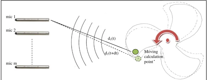
For rotating sources, previous work [1] has demonstrate easily locate sound sources. The

each position of the source (figure .1).

In the equation 1, the rotating motion will change the

Equation 1 becomes :

s P(

with wm(t) the weighting applied on microphones proportional to the distance. This formulation has the advantage to take

to the rotation of the source. This algorithm is suitable for general moving objet like pass by applications.

Data re-sampling

From equation 3, the signal reconstructed at source location will lead to irregular sampled temporal signal on microphone. The best way to

data, and to use a sampling frequency more than

Autospectra exclusion

Equation 3 can be re-written as :

with ( , ) ( ) ( ( c d t P t w t s A m m m m = × +

In practical implementation, before summation over microphone

shift to frequency domain, and the summation is done following the equation : mic 1

mic 2

mic m

previous work [1] has demonstrated the capacity of temporal approach to beamformed signal is processed by calculating reception date for (figure .1).

Figure 1: Near field signal delay

equation 1, the rotating motion will change the ∆m(s) term with time dependenc

c t s d t s m m ) , ( ) , ( = ∆

∑

the weighting applied on microphones proportional to the distance. This formulation has the advantage to take into account the time delays, and the

to the rotation of the source. This algorithm is suitable for general moving objet like pass by

From equation 3, the signal reconstructed at source location will lead to irregular sampled temporal hone. The best way to re-sample signal with good results is to interpolate linearly data, and to use a sampling frequency more than twice the analysis frequency.

∑

In practical implementation, before summation over microphone is achieved, the temporal signal is shift to frequency domain, and the summation is done following the equation :

Moving calculation point d1(t) d1(t+dt) 2

e capacity of temporal approach to signal is processed by calculating reception date for

time dependency : (2)

(3) the weighting applied on microphones proportional to the distance.

the time delays, and the Doppler effect due to the rotation of the source. This algorithm is suitable for general moving objet like pass by

From equation 3, the signal reconstructed at source location will lead to irregular sampled temporal signal with good results is to interpolate linearly

the analysis frequency.

(4)

, the temporal signal is shift to frequency domain, and the summation is done following the equation :

3 ) ( ) ( 2 ) , ²( 0 1 * f A f A f s P M m M m n n m

∑ ∑

In equation 5 the autospectra terms are removed from the summation, it result in the cancelation of microphone self noise which can be electric noise or some real noise like wind noise on the microphone itself.

VALIDATION FOR BOTH MOVING AND STATIONNARY NOISE

Tonal source

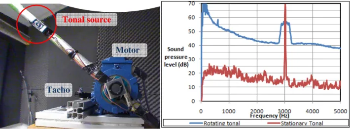
First validation has been done for a tonal source at 3000Hz, this source consists in a small speaker plugged on a signal generator. It is fixed on a motor with a speed of 1000 rpm

Figure 2: Tonal source test setup (left); typical pressure spectrum for rotating and stationary source (right)

In the figure 2, the typical spectrum recorded in front of the source is given. When rotating, a frequency shift is clearly visible, it is due to the Doppler effect. Fixed and rotating measurements have been done for the same source with the same level. Figure 3 shows the spectrum back-propagated on the source, both levels at 3000 Hz are equivalent witch show the capability of the algorithm to estimate correctly the sound pressure level. Outside the sound source frequency, the global spectrum has more level, this is the aerodynamic noise emitted by the system itself (motor and rotating axis). The reconstructed level for rotating source shows that the frequency of the source is now correctly estimated.

Motor Tonal source

Figure 3:

In addition, the figure 3 present the spectrum of the rotating tonal source treated with the stationary algorithm, it appears that the level over the whole frequency band is lower than with the rotating algorithm. It makes possible by comparing the level given by the two algorithm

the sound source is rotating or fixed. Broadband rotating source with

In real fan noise applications, tonal noise often radiates from the blades, fixing elements). To be more close to this case

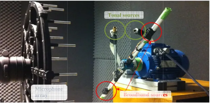
consists in two broadband noise fixed on th be stationary (figure 4). The goal of this both rotating and fixed sources.

Figure 4: Test setup with fixed and rotating sound source in front of the array. 40 45 50 55 60 65 70 75 80 85 90 0 500 1000 Sound pressure level (dB)

Rotating source, rotating processing Fixed source, fixed processing

Microphone array

: Sound pressure estimation at the source location

addition, the figure 3 present the spectrum of the rotating tonal source treated with the stationary it appears that the level over the whole frequency band is lower than with the rotating algorithm. It makes possible by comparing the level given by the two algorithm

the sound source is rotating or fixed.

Broadband rotating source with stationary tonal

In real fan noise applications, tonal noise often radiates from the fixed parts of the fan (counter blades, fixing elements). To be more close to this case, a second experiment

in two broadband noise fixed on the rotating axis, and two other tonal sources e goal of this approach is to show capability of the algorithm to

Test setup with fixed and rotating sound source in front of the array. 1000 1500 2000 2500 3000 3500

Frequency (Hz)

Rotating source, rotating processing Rotating source, fixed processing Fixed source, fixed processing

Tonal sources

Broadband source

4

addition, the figure 3 present the spectrum of the rotating tonal source treated with the stationary it appears that the level over the whole frequency band is lower than with the rotating algorithm. It makes possible by comparing the level given by the two algorithms to understand if

parts of the fan (counter experiment has been done. It e rotating axis, and two other tonal sources which will to show capability of the algorithm to separate

Test setup with fixed and rotating sound source in front of the array.

4000 4500 5000 Rotating source, fixed processing

5

Tonal sources have been tuned to 1800 and 3000 Hz, broadband sources are fixed on the rotating axis, speed for this measurement will be 1500 rpm. Next figure (N°5) shows the average pressure level on the calculation grid.

Figure 5: Average sound pressure level on the calculation grid.

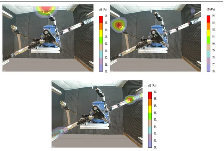
As previously mentioned, by considering that the correct algorithm will give a higher pressure level, it appears that tonal sources are some stationary sources, and broadband noise is rotating noise. The noise around 10 kHz, comes from the electric motor itself, so it is also stationary noise.

Figure 6: Acoustic hologram fixed tonal source 1800 Hz (top left), tonal 3000 Hz (top right), and rotating broadband noise (bottom). 0 10 20 30 40 50 60 70 0 2000 4000 6000 8000 10000 12000 14000 Average pressure level (dB) Frequency (Hz)

Our case concerns an industrial fan use

axial fan with 11 blades on the rotor, and 31 blades on the stator. Rotor diameter is around 200 mm, and rotational speed around 10000 RPM.

Figure

Validation of the algorithm for high rotational speed The goal of the first measurement is

(counter clockwise), it consists in two o assumed to be noisy.

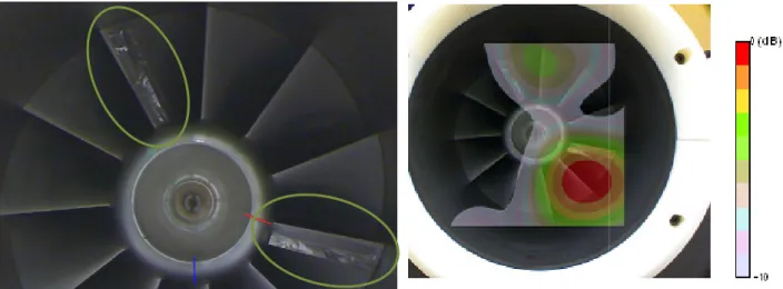
Figure 8: Obstacles on blades

Those obstacles are shown in figure 8, they are fixed just after the leading edge of the blade. Angle between the two blades has been c

array. Hologram is presented in figure 8, for the two obstacle on the following blade at its tip

measurement at 5000 RPM has been done

CASE STUDY ON A FAN

an industrial fan used in aeronautics industry for air extraction. It consist

axial fan with 11 blades on the rotor, and 31 blades on the stator. Rotor diameter is around 200 mm, and rotational speed around 10000 RPM. The fan is mounted inside a duct.

Figure 7: Test setup at the ISAE test bench.

m for high rotational speed

The goal of the first measurement is to validate the processing for a 10000 RPM rotational speed in two obstacles fixed on two blades, which produce

Obstacles on blades(left), and sound source localization (right)

are shown in figure 8, they are fixed just after the leading edge of the blade. Angle between the two blades has been chosen to avoid amplifying reflection or seco

Hologram is presented in figure 8, for the two obstacles, it is clear that the source is created on the following blade at its tip area. To confirm this behavior which seems possible, a second measurement at 5000 RPM has been done and gives the same localization.

6

in aeronautics industry for air extraction. It consists in an axial fan with 11 blades on the rotor, and 31 blades on the stator. Rotor diameter is around 200 mm,

for a 10000 RPM rotational speed , which produce a stall and are

(left), and sound source localization (right)

are shown in figure 8, they are fixed just after the leading edge of the blade. Angle reflection or secondary lobe of the , it is clear that the source is created To confirm this behavior which seems possible, a second

7

Standard fan analysis

In [2] Alain Guédel gives some rules about the noise sound generation on fans. Considering that in our case, we may find the blade pass frequency and its harmonics as stationary sources radiating near the stator blades, and we may also find some broadband noise as rotating source on the trailing edge

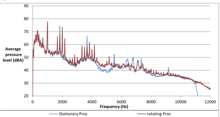
Figure 9: Pressure level on calculation grid with and without rotating processing

Figure 9 present the spectrum for both stationary and rotating processing. Considering that the maximum level is found on the correct algorithm, it is possible to know if sources are rotating or not. A nice improvement of this approach would be to filter stationary tonal signal on microphone before doing the rotating treatment.

Figure 10: Hologram with rotating processing, in frequency range 4500-5500Hz

Figure 10 is the rotating processing done around 5000 Hz, it clearly shows the trailing edge of each blade. 20 30 40 50 60 70 80 90 0 2000 4000 6000 8000 10000 12000 Average pressure level (dBA) Frequency (Hz)

Stationary Proc rotating Proc

dBA (Pa) 86. 87. 88. 89. 90. 91. 92. 93. 94. 95. 96.

8

CONCLUSION

Validations measurements has shown the possibility of our algorithm to analyze rotating sources, and to separate stationary of rotating ones. The test case on a "in duct fan", has shown its capability to correctly track a high speed fan. For further analysis on such device, green functions (in free field condition in our application) has to be estimated closer to the real environment.

BIBLIOGRAPHY

[1] P. Sijtsma, S. Oerlemans, H. Holthusen – Location of rotating sources by phased array measurements, 7th AIAA/CEAS Aeroacoustics Conference, Maastricht, 2001

[2] A. Guédel – Acoustique des ventilateurs - Génération du bruit et moyen de réduction. Editions PYC LIVRES, 1999