Fast aggregation of Student mixture models

HAL Id: inria-00383948

https://hal.inria.fr/inria-00383948

Submitted on 29 Oct 2014

HAL is a multi-disciplinary open access

archive for the deposit and dissemination of

sci-entific research documents, whether they are

pub-lished or not. The documents may come from

teaching and research institutions in France or

abroad, or from public or private research centers.

L’archive ouverte pluridisciplinaire HAL, est

destinée au dépôt et à la diffusion de documents

scientifiques de niveau recherche, publiés ou non,

émanant des établissements d’enseignement et de

recherche français ou étrangers, des laboratoires

publics ou privés.

Fast aggregation of Student mixture models

Ali El Attar, Antoine Pigeau, Marc Gelgon

To cite this version:

Ali El Attar, Antoine Pigeau, Marc Gelgon. Fast aggregation of Student mixture models.

Euro-pean Signal Processing Conference (Eusipco’2009), Aug 2009, Glasgow, United Kingdom. pp.312-216.

�inria-00383948�

FAST AGGREGATION OF STUDENT MIXTURE MODELS

Ali El Attar, Antoine Pigeau and Marc Gelgon

Nantes university, LINA (UMR CNRS 6241), Polytech’Nantes rue C.Pauc, La Chantrerie, 44306 Nantes cedex 3, France

phone: + (33) 2 40 68 32 57, fax: + (33) 2 40 68 32 32, email: firstname.lastname@univ-nantes.fr

ABSTRACT 1. INTRODUCTION

Probabilistic mixture models form a mainstream approach to unsupervised clustering, with a wealth of variants pertaining to the form of the model, optimality criteria and estimation schemes.

Clustering vs density estimation : via criterion (NEC,Biernacki) or via form of model. This paper : latter option, Student. Mixture of Students : exists (citer ML ; pb estimer le degr de liberts. Bayesian, including efficient vari-ational estimation - Archambeau).

Many computation contexts involve handling of multi-ples models of the same process and aggregating them for improving their performance. Both for supervised (boosting) clustering of distributed data (citer qqs papiers).

In particular, multiple partitions of data represented. 2. THE CLUSTERING ALGORITHM

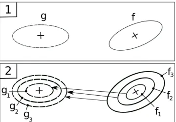
Figure 1: Reduction of a mixture model with [2] : dotted and solid ellipses represent respectively the g and f models. (1) shows the first step where the divergence between compo-nents of g and f are computed (see arrows). (2) presents the parameter update of g based on the mapping m, minimizing the criterion 1.

The algorithm [2] proposes to reduce a large Gaussian

model f into a smaller model g while preserving the initial structure. The particularity of the task is due to the sole use of model parameters to regroup the components. The algorithm minimizes a distance between f and g defined as:

d( f , g) = K

∑

where K and M are respectively the number of components of f and g, πiis the mixing proportion of the Gaussian

com-ponent i and KL is the Kullback Leibler divergence.

Similar to the k-means algorithm, the optimization pro-cess is divided in two steps. The first one is to determine the association of components between f and g minimizing equation 1. Practically, it amounts to determine the best map-ping m from{1 . . . K} to {1 . . . M} such that the criterion (1) is minimized: d( f , g) = d′( f , g, m) = K

∑

where the function KL is an approximation of the Kullback Leibler divergence defined as:

KL( fi||gi) = 12[log |Σ_gi| |Σ_fi|+ Tr|Σ−1gi Σfi| −d + (µfi− µgi) t_Σ−1 gi (µfi− µgi)] (3) where d is the dimension.

The second step is to update the model parameters of g. These parameters are re-estimated from the sole model pa-rameters of f .

These two steps are iterated until the convergence of the criterion defined in equation 1. Figure 1 depicts the cluster-ing algorithm.

Adaptation of this algorithm to a Student mixture raises two distinct problems. First, to our knowledge, it does not exist any analytic solution to compute the Kullback Leibler divergence between two Student components. We propose then a new approximation of the Kullback Leibler diver-gence, based on a decomposition of a Student component with a finite sum of Gaussian component. Second, and this problem results from our proposed approximation, the up-date of model parameters (step 2) is adapted.

The algorithm 1 summarizes the different steps of our approach.

2.1 Approximation of the Student distribution

The Student distribution is defined by an infinite sum of Gaussian distributions with a similar mean and different co-variance values:

f(x, µ, Σ, ν)st=

Z ∞

0

Algorithm 1 Clustering algorithm

Require: two Student mixtures f and g, respectively of K and M components (K> M). Means of g are initialized randomly and the pth_{(1 < p < P) covariance is set to the}

identity matrix pth

1.Approximate each Student component of f and g with P Gaussian components

while d( f , g) is not minimized do

2.1.compute the Kullback Leibler divergence approxi-mation between the components of f and g.

2.2.update the model parameters of g based on the map-ping functions m and m′.

end whilethe model g, which is the reduction of the model f −100 −8 −6 −4 −2 0 2 4 6 8 10 0.05 0.1 0.15 0.2 0.25 0.3 0.35 0.4 v = 30 v = 1 v = 0.1

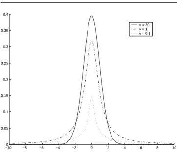
Figure 2: Student density for several values of the degrees of freedom. As ν→ ∞, the distribution corresponds to a Gaus-sian. For a low degree of freedom, the heavy tails involves more robustness face to outliers.

where N (x, µ, Σ/u) is a Gaussian component with mean µ and covariance Σ, ν is the degrees of freedom and G is the the Gamma distribution. Figure 2 presents the curve of a Student distribution in accordance with the degrees of freedom.

The term u of equation 4 can be interpreted as follows: it represents the covariance’s weight of each Gaussian com-ponent. Knowing this, a fair solution to obtain an analytic solution for an approximated KL is to randomize a finite set of P Gaussian components in accordance with the distribu-tion of u. Our Student approximadistribu-tion is then defined as a sum of P Gaussian components: fst(x) = K

∑

∑

Figure 3 presents an example on our approximation of a Stu-dent component with 3 Gaussian components.

Notice that the number P of Gaussian components to ap-proximate a Student distribution depends of ν. Indeed, when ν→ ∞, the distribution corresponds to a Gaussian compo-nent: the higher is ν, the lower should be P. Our experiments confirm this point.

Figure 3: Left figure presents the Gamma distribution of the term u. We select randomly a finite sum of Gaussian components to represent the Student distribution (here three terms u1, u2and u3). Right figure shows the selected

Gaus-sian components (gray lines) to approximate the Student one (black line).

2.2 Kullback Leibler divergence between two Student approximations

Our Gaussian representation of a Student component gives us the opportunity to use an approximation of the Kullback Leibler divergence between Gaussian mixture. Several ap-proaches were compared in [3]. Sampling method based on the Monte Carlo are of course proposed, leading to the best result, but presents the disadvantage of an high calculation complexity. Methods based on models parameters are then a good compromise between the quality and the cost, in term of calculation complexity, of the approximation. Experiments in [3] conclude that, among the approximation methods, the best approaches are the matched bound and the variational approximations. Because this latter needs a costly optimiza-tion with an EM procedure, our choice fells on the matched bound criterion [1].

This approximation of the Kullback Leibler divergence between two models f and g is very similar to the previous criterion 2, also based on a mapping function m′minimizing the sum of Kullback Leibler divergences:

KL_matchBound( f ||g) =

_∑

Approximation of a Kullback Leibler divergence be-tween two Student components amounts then to compute the Kullback Leibler divergence between two Gaussian models, both composed of P components and a similar mean. Fig-ure 4 shows an example of our method to compute an ap-proximate Kullback Leibler divergence between two Student components.

Once the Kullback Leibler divergence obtained for each approximate Student between f and g, each component of g can be assigned to the closest components of f . Parameters of g are then updated in accordance with the mappings m and m′.

2.3 Update of the model parameters

Initially proposed for Gaussian components, the parameter update of [2] need to be adapted to deal with our approxi-mation of Student components. [2] proposed to compute the average of the mean and the covariance in accordance with

Figure 4: Example of the Kullback Leibler divergence be-tween two approximate Student components. Solid and dot-ted lines represent respectively the models f and g. On figure (1) the original Student components. On figure (2), our pro-posed approximation of the Student component with P= 3 Gaussian components. Optimization of the matched bound criterion amounts to map the components of f and g such that the sum of the Kullback Leibler divergences is minimized. Here, the arrows show the obtained mapping m′. Note that the mapping is not necessarily surjective.

the mapping m obtained at previous step. Our approach is similar to assign a Student approximation of g to f , but in-clude a new inner step to update the parameters of its Gaus-sian components. Each GausGaus-sian is updated in accordance with its m′−1associated Gaussian component from the m−1 component of f . Let j a Student component of g assigns to ncomponents of f . Its parameters are updated as follows:

µj= 1 πj_i∈m

∑

∑

∑

Its single center is the average of the n center of f . Each one of its P covariances is the average of the associate co-variance of f , based on the mapping m′.

Note that since m′is not surjective, a covariance Σj pcan

be associated to none covariance among the n covariances of f. In this case, we update it with the average of n covari-ances, one per associated components of f , minimizing their Kullback Leibler divergence.

3. EXPERIMENTS

To validate our proposal, we first compute a KL divergence between a Student and our approximation for different num-ber of Gaussian components. Then we propose an example of a Student model reduction with our adapted algorithm.

For our first experiment, we sample 5000 data in accor-dance with a Student distribution and compute the KL diver-gence based on the Monte Carlo method. For p varying from 1 to 50, we carried out the following steps, 20 times each:

0 10 20 30 40 50 0 2 4 6 8

Number of Gaussian components

KL divergence df=0.3 df=0.8 df=2 df=4 df=8 df=15

Figure 5: KL divergence between our approximation and the Student distribution according to the number of components and the degrees of freedom. As this latter increased, the num-ber of needed components to obtain a low KL divergence de-creased. This is explained by the fact that the distribution tends to a Gaussian when v→ ∞.

• select the p Gaussian components: randomize p values of term u in accordance with the Gamma distribution • compute the KL divergence

The average KL divergence for the 20 iterations are plotted on Figure 5, for various values of ν.

This experiment confirms that as ν increases, the number of components to obtain a low KL divergence decreases. In-deed, for ν≥ 2, the associated curves tend quickly to 0 giving a good approximation for p varying between 8 and 20 com-ponents. For a smaller value of ν, the result is more chaotic, involving an optimization of the divergence for nearly 40 Gaussian components.

REFERENCES

[1] J. Goldberger, S. Gordon, and H. Greenspan. An efficient image similarity measure based on approximations of kl-divergence between two gaussian mixtures. In Proceed-ings of Ninth IEEE International Conference on Com-puter Vision, volume 1, pages 487–493, 2003.

[2] J. Goldberger and S. Roweis. Hierarchical clustering of a mixture model. In Advances in Neural Information Pro-cessing Systems 17, pages 505–512, Cambridge, MA, 2004. MIT Press.

[3] J. R. Hershey and P. A. Olsen. Approximating the kull-back leibler divergence between gaussian mixture mod-els. In Acoustics, Speech and Signal Processing, 2007. ICASSP 2007. IEEE International Conference on, vol-ume 4, pages IV–317–IV–320, 2007.