Robust ensemble learning framework for day-ahead forecasting of household based energy consumption.

1

Robust ensemble learning framework for day-ahead forecasting of

household based energy consumption

1 _{Department of Civil Engineering and Applied Mechanics, McGill University, 817 Sherbrooke Street West,} Montréal (QC), H3A 2K6, Canada

2 _{Eau Terre Environnement, Institut National de la Recherche Scientifique, 490 Rue de la Couronne, Québec (QC),} G1K 9A9, Canada

*_{Corresponding author; Email: mohammad.alobaidi@mail.mcgill.ca}

Abstract

Smart energy management mandates a more decentralized energy infrastructure, entailing energy consumption information on a local level. Household-based energy consumption trends are becoming important to achieve reliable energy management for such local power systems. However, predicting energy consumption on a household level poses several challenges on technical and practical levels. The literature lacks studies addressing prediction of energy consumption on an individual household level. In order to provide a feasible solution, this paper presents a framework for predicting the average daily energy consumption of individual households. An ensemble method, utilizing information diversity, is proposed to predict the day-ahead average energy consumption. In order to further improve the generalization ability, a robust regression component is proposed in the ensemble integration. The use of such robust combiner has become possible due to the diversity parameters provided in the ensemble architecture. The proposed approach is applied to a case study in France. The results show significant improvement in the generalization ability as well as alleviation of several unstable-prediction problems, existing in other models. The results also provide insights on the ability of the suggested ensemble model to produce improved prediction performance with limited data, showing the validity of the ensemble learning identity in the proposed model. We demonstrate the conceptual benefit of ensemble learning, emphasizing on the requirement of diversity within datasets, given to sub-ensembles, rather than the common misconception of data availability requirement for improved prediction.

Keywords: household energy consumption; ensemble learning; robust regression; day-ahead energy

2

1. Introduction and Motivation

The demand for energy is continuously rising and, consequently, leading to unsustainable exhaustion of the nonrenewable energy resources. The increase in urbanization have led to an increase in electricity consumption in the last decades [1-3]. Many countries are continuously moving toward decentralized power systems; therefore, the use of distributed generation of electrical energy instead of the traditional centralized system is becoming popular [4-8]. To face the growing electricity demand and reinforce the stability of this new energy infrastructure, a more decentralized microgrid represents the key tool to improve the energy demand and supply management in the smart grid [9, 10]. This is achieved via utilizing information about electricity consumption, transmission configuration and advanced technology for harvesting renewable energy on a finer demand/supply scale. These systems are expected to improve the economy and deliver sustainable solutions for energy production [11, 12].

Furthermore, power balance is one of the major research frontiers in decentralized energy systems; the high penetration levels of renewables prompt additional demand-supply variability which may lead to serious problems in the network [13, 14]. Also, the relatively small scale of new decentralized energy systems highlights the importance of predicting the demand projections, which are not similar to the demand projections in the main grid and impose additional variability in the net-load of the system [9, 15]. Hence, short-term load forecasting at the microgrid level is one of the critical steps in smart energy management applications to sustain the power balance through proper utilization of energy storage and distributed generation units [3, 16, 17]. Day-ahead forecasting of aggregated electricity consumption has been widely

Nomenclature

ANFIS adaptive neuro fuzzy inference system MLR multiple linear regression ANN artificial neural network OLS ordinary least squares BANN ANN based bagging ensemble model RBF radial basis functions

DT decision tree rBias relative bias error

EANN proposed ensemble framework RF-MLR robust fitting based MLR

KF kalman filter RMSE root mean square error

MAD median absolute deviation rRMSE relative RMSE MAPE mean absolute percentage error SANN single ANN model MDEC mean daily electricity consumption SCG scaled conjugate gradient

3 studied in the literature; however, forecasting energy consumption at the customer level, or smaller aggregation level, is much less studied [13, 18]. The recent deployment of smart meters helps in motivating new studies on forecasting energy consumption at the consumer level [11, 13, 19]. On the other hand, forecasting energy consumption at smaller aggregation level, down to a single-consumer level, poses several challenges. Small aggregated load curves are nonlinear and heteroscedastic time series [13, 20, 21]. The aggregation or smoothing effect is reduced and uncertainty, as a result, increases as the sample size of aggregated customers gets smaller. This is one of the major issues leading to the different challenges in household-based energy consumption forecasting. The studies in [22-24] discuss the importance and the difficulties in forecasting the energy consumption at the household level.

Further, the behavior of the household energy consumption time series becomes localized by the consumer behavior. Additional information on the household other than energy consumption, such as household size, income, appliance inventory, and usage information can be used to further improve prediction models. Obtaining this information is very difficult and poses several user privacy challenges. For example, Tso and Yau [25] achieve improved household demand forecasts by including information on available appliances and their usage in each household. The authors describe the different challenges in attaining such information via surveying the public. As a result, innovating new models that can overcome prediction issues with the limited-information challenge is indeed one of the current research objectives in this field. In short-term forecasting of individual households’ energy consumption, ensemble learning can bring feasible and practical solutions to the challenges discussed earlier. Ensemble learners are expected to nullify bias-in-forecasts, stemming from the limited features available to explain the short-term household electricity usage. However, to the best of our knowledge, there has not been much work done on utilizing ensemble learning frameworks for the problem at-hand.

This work focuses on the specific problem of practical short-term forecasting of energy consumption at the household level. More specifically, we present a proper ensemble-based machine learning framework for day-ahead forecasting of energy consumption at the household level. The study emphasizes on the

4 successful utilization of diversity-in-learning provided by the two-stage resampling technique in the presented ensemble model. This ensemble framework allows for utilizing robust linear combiners, as such combiners are not used before due to the unguided overfitting behavior of the ensemble model in the training stage. The results of the study focus on the ability of the presented ensemble to produce improved estimates while having limited amount of information about the household energy usage history (in terms of variables and observations available for the training).

This paper is organized as follows; Section 2 presents a concise background on common techniques for forecasting of energy consumption as well as the significance of ensemble learning in such case studies. In Section 3, we introduce the methodology of the proposed ensemble. Section 4 is devoted to an application of our method to mean daily household energy forecasting. The case study in this paper and the comparison studies are given in this section as well. The discussion of the results is provided in Section 5, and concluding remarks are given in Section 6.

2. Background and Literature Review

A summary of the methods commonly used in the literature for forecasting energy consumption is presented. Table 1 provides an overview of the advantages and disadvantages of the different categories of models discussed in this section. Common techniques for energy consumption forecasting include time series models [26], Exponential Smoothing [27], Linear Regression [28], Generalized Additive Models [29, 30], and Functional Data Analysis [13]. Such classical methods, also referred to as non-machine learning methods, have been comprehensively studied in the literature, and a useful overview of their common attributes can be found in [31]. The previously mentioned techniques have been demonstrated on aggregated demand studies. On the other hand, such techniques are expected to yield unsatisfactory results at the household level due to the challenges in the individual household energy usage patterns [32, 33]. Instead, the limited literature on forecasting household-level (not aggregated) energy consumption suggests machine learning techniques.

5 Table 1: General characteristics of classical, single and ensemble machine learning models (not only for energy applications).

Broad

Group Attributes and Advantages Weaknesses and Disadvantages

Non-Machine Learning Methods

- Common and well established in the wide literature.

- Perform well in forecasting aggregated load time series at different temporal resolutions. - Provide statistical significance of prediction. - Usually quantify uncertainty in obtained

predictions.

- Fast-Implementation to any case study.

- Poor performance in forecasting short-term complex time series.

- Dependence of various assumptions which may be very unreliable.

- Limited ability to utilize additional variables in the prediction model.

- Sensitivity to correlations within explanatories. - Curse of dimensionality.

Single Machine Learning Methods

- Do not require assumptions on the nature of variables.

- Increasingly accepted methods for various applications in the literature.

- More flexible methods that can fit better to complex time series.

- Can accommodate different variables in time series forecasting.

- Often provide better generalization ability than classical methods.

- May be computationally more expensive than classical methods.

- In time series forecasting, mostly used for curve-fitting objectives rather than statistical

interoperability of predictions.

- Fitting-behaviour of many methods are still poorly understood.

- Curse of dimensionality.

- Inherent instability in the learning of a case study, even with similar training configurations.

Ensemble Machine Learning Methods

- Do not require assumptions on the nature of variables.

- Very flexible methods that can provide the best fitting approaches.

- Enjoy far more stable performance than single modeling frameworks.

- Can provide information on uncertainty. - Can significantly reduce the effect of

dimensionality; high dimensional systems are handled better without significant impact on performance.

- Relatively new learning frameworks.

- Learning in-series may create computationally expensive methods.

- Mostly available for classification problems rather than regression.

- Diversity concept, contribution to its generalization ability, is not usually tackled in an explicit manner in many of the common ensemble models. - Generalized learning frameworks require careful

consideration when applied to a definite field and a certain case study.

Machine Learning in Forecasting Energy Consumption

Examples of machine learning models are Support Vector Machines (SVMs), Adaptive Neuro-Fuzzy Inference Systems (ANFISs), Kalman Filters (KFs), Decision Trees (DTs), Radial Basis Functions (RBFs) and Artificial Neural Networks (ANNs) [3, 34-37]. The literature is abundant with research studies stating that machine learning models significantly outperform the classical statistical methods [38, 39]. For example, Pritzsche [40] compares machine learning models to classical ones and shows that the former can significantly improve forecasting accuracy in time series. In the specific literature of forecasting electricity consumption, the work in [25] utilizes DTs in predicting energy consumption levels. The use of KF is

6 proposed in [41]. It is critical to note that the two previous studies use a large dataset of consumers, not individuals, but refer to the work as household energy forecasting. In addition, the earlier study relies on household appliance information, which is a significantly impractical requirement to build prediction models. In [36], the authors demonstrate a forecasting approach using SVM applied on a multi-family residential building. Also, SVMs and ANNs are adopted for household energy forecasting in [42]. However, the study focuses on determining the optimum aggregation size of households rather than energy consumption forecasts. A more recent study by Xia et al. [43] develops wavelet based hybrid ANNs in electrical power system forecasting, which can be applied to forecast electricity price or consumption. The results of the study show a significant improvement in the generalization ability of this model when used to forecast power system states. Nevertheless, wavelet based machine learning techniques are expected to provide a deteriorated performance when individual-human behavior becomes a driving variable to the power system. In other word, decomposing the individual household electricity consumption time series is expected to provide misleading patterns that are not useful for daily load forecasting.

The day-ahead average energy consumption forecasts of individual households are important for a wide variety of real life applications. For example, household energy forecasts on a daily basis can support wholesale electricity market bidding, where the load serving entity may submit a fixed Demand Response offer curve that is constructed from knowledge of the day-ahead average energy consumption of individual smart homes [44]. In addition, day-ahead average energy consumption can benefit the energy storage of relatively small and islanded power systems, down to a household level [45]. Also, this forecasting problem has recently been targeted in estimating greenhouse gas emissions and short-term carbon footprints of individual households [46].

Perhaps the alluring nature of machine learning is also considered one of its major drawbacks. More precisely, machine learning models are instable learners; optimization of a certain model can yield different optimum configurations, even with the same training and validation environment. In the case of ANNs, this instability manifests in the random initiation of the hidden neuron’s weights, required to start the training

7 stage, which leads to different local optimum solutions for the model. This suggests that such instability can negatively affect the generalization ability of machine learning models if certain inferior conditions exist in the variables considered or in the data available for training and validation. To this extent, ensemble learning is a recent advancement to common machine learning techniques, and has been suggested over a wide spectrum of applications in the literature [47-50].

Common Ensemble Models in the General Literature

The main advantages of ensemble models, compared to single models, are depicted in their improved generalization ability and flexible functional mapping between the system’s variables [51, 52]. Figure 1 depicts the common architecture of ensemble models, in a homogeneous-learning setting where the sub-ensemble processes are similar. Hybrid sub-ensembles, also called Nonhomogeneous or Heterogonous ensembles, comprise a combination of different models. Ensemble learning commonly comprises three stages [34] which are resampling, sub-model generation and pruning, and ensemble integration. Resampling, which deals with generating a number of data subsets from the original dataset, is often the main character behind a key-ensemble model, as described later. Sub-model generation defines the process of choosing a number of appropriate regression models for the system at-hand. Pruning the sub-models (or ensemble members) determines the optimum ensemble configurations and the sub-models’ structures. Lastly, ensemble integration is the specific technique that transforms or selects estimates coming from the members, creating the ensemble estimate.

The most common ensemble learning frameworks throughout the applied science literature are Bagging [53], Generalized Stacking [54] and Boosting [55]. These ensembles can be used to in a Homogeneous as well as Nonhomogeneous (Hybrid) setting. Bagging ensembles, for example, employ Bootstrap resampling to generate the subsets and use a mean combiner to create the ensemble estimates. A wide variety of machine learners can be used as ensemble members, whereas this is a common feature to all ensemble models rather than Bagging. Stacked Generalization (or Stacking) is a two-level learner, where resampling

8 and model generation and training are done as a first level training stage in the ensemble process. The second level training stage is the generation of the ensemble integration, which is a weighted sum of the members’ estimates.

While Bagging and Stacking are viewed as ensembles with parallel learning framework (i.e. individual members can be trained independent from each other), Boosting is an in-series ensemble that creates members, in a receding horizon, based on the performance of the previous members in predicting all the observations in the training set. The first member will take in the observations of the original sample set as observations with the same probability of occurrence, and the observations with poor estimates will prompt an informed change in the whole sample to shift the focus of training toward such observations in succeeding ensemble members. For more information about ensemble learners, a survey of common ensemble techniques in the machine learning literature can be found in [48, 56].

The main advantages of ensemble models, compared to single models, are depicted in their improved generalization ability and flexible functional mapping between the system’s variables [51]. Figure 1 depicts the common architecture of ensemble models, in a homogeneous-learning setting. Ensemble learning commonly comprises three stages [34] which are resampling, sub-model generation and pruning, and ensemble integration. Resampling, which deals with generating a number of data subsets from the original dataset, is often the main character behind a key-ensemble model, as described later. Sub-model generation defines the process of choosing a number of appropriate regression models for the system at-hand. Pruning the models (or ensemble members) determines the optimum ensemble configurations and the sub-model’s structure. Lastly, ensemble integration is the specific technique that transforms or selects estimates coming from the members, creating the ensemble estimate.

9 Figure 1: Typical ensemble learning frameworks specific to homogeneous ensemble models; a) In-Series Learning, native

to Boosting ensembles; b) Parallel Learning, as in Bagging ensembles.

Diversity Concept

The main attribute of ensemble learning, in which the improved generalization ability is manifested, is theorized to be the diversity-in-learning phenomenon. Diversity is simply the amount of disagreement

10 between the estimates of the sub-models [58, 59]. One major source of ensemble diversity is the nature of the resamples in the training stage. When the resamples are created for the members’ training, the relative uniqueness of the information available in each subset prompts the members to capture different patterns along the system dynamics. While infrequently highlighted in the literature, the concept of diversity is not directly tackled in the most employed ensemble methods and is commonly of-interest for classification-based studies rather than the regression [60, 61].

In regression settings, the realization of diversity effects on the ensemble generalization ability has been implied by Krogh and Vedelsby [62], as the variance in estimates by the ensemble members. The authors also suggest that an ensemble whose architecture successfully increases ensemble diversity, while maintaining the average error of the sub-models, should have an improved generalization ability, in terms of mean squared error of the ensemble estimates. Ueda and Nakano [63] extend the previous work to derive an explicit description to ensemble diversity, manifested in the bias-variance-covariance decomposition of a model’s expected performance. This notion is the main reason behind the common preview “the group is better than the single expert” and becomes an identity, defining a proper ensemble. More recently, Brown et al. [64] develop a diversity-utilizing ensemble learning framework, which is inspired from an ANN learning technique [65]. The authors show that an error function for each individual can be derived by taking the ensemble integration stage into account, enabling explicit optimization of ensemble diversity. The authors also show that resultant ensemble models provide improved generalization over many case studies when compared with common ensemble learners, such as Bagging.

In this work, a robust ensemble learning framework is presented. One of the major characteristics of the presented model is the direct utilization of ensemble diversity investigation in the training process. This diversity is created from the first ensemble learning component, the resampling technique. It is expected that creating diverse resamples will prompt the whole model to become diverse. The novelty in the presented model is its ability to measure diversity, via introducing information mixture parameters, without affecting the random learning character of the training stage. In addition, the suggested ensemble can utilize

11 linear combiner as ensemble combiner, unlike common ensemble learners. This enables the addition of a robust combiner, which significantly contribute to the prediction accuracy of the problem at-hand.

Furthermore, ANNs are selected in this study as sub-ensembles, or ensemble members, due to their resiliency in generating diverse realizations, facilitating the resampling plan to create the expected diversity in the ensemble learner [49, 66]. The bias-variance-covariance composition of ANN-based ensemble models have been studied in the literature. They show many benefits of ANNs as ensemble members [38, 58, 62]. More recent, the work by Mendes-Moreira et al. [48] provides a survey on ensemble learning from diversity perspective and concludes that the most successful ensembles are those developed for unstable learners that are relatively sensitive to changes in the training set, namely Decision Trees and ANNs. The next section provides a detailed overview of the proposed model.

3. Methodology

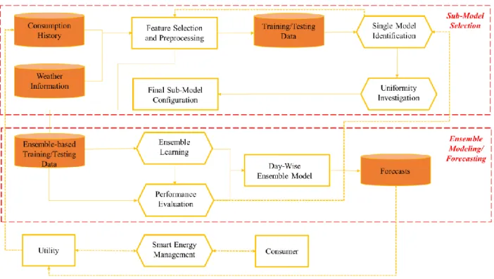
In general, the three main stages that make up ensemble learning are: resampling, sub-ensemble generation and training, and ensemble integration. A certain ensemble learning framework utilizes a method in one or more of these three stages, unique to that ensemble. In this work, an ensemble-based ANN framework with minute-controlled resampling technique and robust integration is proposed. In addition, an ensemble model is constructed using the proposed framework to estimate the day-ahead average energy consumption for individual households. Figure 2 summarizes the ensemble learning process presented in this work. From a machine learning perspective, the novelty in the presented ensemble learning framework exists within the first and third ensemble learning stages; the developed two-stage resampling technique utilizing diversity within the ensemble members allow explicit diversity-control within the resamples and, consequently, the sub-ensemble models. Also, the ability of the presented ensemble framework to exploit robust linear combiners for the ensemble integration stage is unique, compared to common ensemble frameworks.

12 In this section, the description of the ensemble learning methodology follows a systematic process that takes into consideration the ensemble identity, namely resampling, model generation and pruning, and sub-ensemble integration. Also, the methodology is designed to describe the utilized techniques in resampling and ensemble integration because the proposed ensemble model is unique in these two stages.

Figure 2: Comprehensive methodology to the ensemble learning process within a potential application. The dashed arrows indicate processes that are out of the scope of the current paper.

The Two-Stage Resampling Plan

The resampling plan consists of a two-stage diversity controlled random sampling procedure. In the first stage, the dataset is divided into k resamples, where k is the size of the ensemble model (i.e. number of sub-models in the ensemble). These resamples are referred to as first-stage resamples, and are described as follows: 𝑛1 = 𝑁 − 𝑛_{𝑏𝑙𝑜𝑐𝑘𝑒𝑑} 𝑘 = 𝑁 (1 − 𝑚_𝑐) 𝑘 , 1 ≤ 𝑘 ≤ (𝑁 − 𝑛𝑏𝑙𝑜𝑐𝑘𝑒𝑑), (1)

13 where 𝑛1 is the first-stage subsample size, and 𝑛𝑏𝑙𝑜𝑐𝑘𝑒𝑑 is the number of the blocked observations from the

training sample, N is the size of the sample set available for the training, and 𝑚_𝑐 is the mixture ratio used to determine the amount of blocked information which will be utilized in the training of the linear ensemble combiner.

Typically, 𝑚_𝑐 can vary between 10% and 30%, depending on the availability of training data, the ensemble size, and the nature of the ensemble combiner used. A simple random sampling without replacement is used to pick out the samples for the purpose of blocking them from the members’ training. Although the resamples have the same size, each subsample will have different observations from each other; no observation can be found in more than one first-stage subsample.

The second-stage resamples are then generated by random, but controlled, information exchange between all the first-stage resamples. Using a parameter that controls the amount of information mixture in each resample, a certain number of observations is given from one resample to another. In this work, the mixture-control parameter is utilized in the generation of the second-stage resamples as follows:

𝑛_2𝑖 = 𝑛_1𝑖+ ∑ 𝑚_𝑒× 𝑛_1𝑗

𝑘 𝑗=1 𝑗≠𝑖

, ₍₂₎

where 𝑛_2𝑖 is the size of the ith _{second-stage resample, 𝑚}

𝑒 is the information-mixture ratio, 𝑛1𝑗 and 𝑛1𝑖 are

the size of the jth and of the ith first-stage subsample, respectively (𝑖, 𝑗 = 1,2,3, . . , 𝑘). It is worth noting that although all first-stage and consequent second-stage resamples have the same size, the subscripts i and j are added in order to emphasize the fact that the first-stage resamples hold different information.

The mixture ratio, 𝑚_𝑒, should vary between 0 and 1. The value 0 means that the second-stage resamples are the same as the first-stage resamples (no information-mixture). The value 1 means that all the second-stage resamples have the same observations in the original dataset (and have the same size). Figure 3

14 presents the relationship between the information-mixture and the ratio of the second-stage resamples to the net sample set. It is expected that the optimum resamples (i.e. prompts the best ensemble learning performance) lie somewhere between the two values. In addition, the zero-mixture downgrades diversity-in-learning, and the saturation of the second-stage resamples (𝑚_𝑒= 1) implies that diversity will only arise from the individual member models rather than the training resamples. Consequently, the mixture ratio, for all the second-stage resamples, is defined as:

𝑚_𝑒= 𝑛𝑠ℎ𝑎𝑟𝑒𝑑𝑗

𝑛_1𝑗 , 0 ≤ 𝑛𝑠ℎ𝑎𝑟𝑒𝑑𝑗≤ 𝑛1𝑗, (3)

where 𝑛_{𝑠ℎ𝑎𝑟𝑒𝑑𝑗} is the number of observations shared by the jth first-stage resample, and 𝑛1𝑗 is the size of

the same resample. Notice that equation (4) states that the jth _{homogeneity ratio, 𝑚}

𝑒, will have a value

between 0 and 1, bounding the amount of information shared by the jth first-stage resample in order not to exceed its size (preventing redundancy in shared information). In addition to the diversity reasoning behind the mixture ratio, equation (4) distinguishes the proposed resampling technique from that suggested in the common Bagging ensembles. The information-mixture ratio 𝑚_𝑒 can be optimized for a given case study by a validation plan, where a set of mixture ratio values is defined and used to generate the resamples. The effect of the resamples on the overall ensemble performance is then investigated for each value, discussed in the following section.

Sub-Ensemble Models

After the resamples are prepared, sub-ensemble models are created and trained using the resamples. The choice of the ensemble members (sub-ensemble members) depends on the type of the problem, available variables as well as the dataset itself. In this paper, the ensemble members used are ANN. Multi-Layer Perceptron (MLP) Feed-Forward ANN is well established in the literature and detailed information about this model can be found in [34, 66]. Hence, discussing MLP-based ANNs is not necessary. However, optimum design of ANN-based ensemble architecture (parameter selection) is discussed in the next section.

15 The Scaled Conjugate Gradient (SCG) is used as the training algorithm for the ANNs [67]. SCG has been shown to provide satisfactory learning performance to ANNs with relatively complex inputs [68, 69].

Figure 3: Relationship between the information-mixture parameter and the amount of information contained in the second-stage resamples.

The ensemble size, k, plays a major role in the proposed resampling plan, as it determines the size of the first-stage resamples and the size of the shared information, along with the mixture ratios in the second-stage resamples. On the other hand, determining the optimum number of sub-models, i.e. the ensemble size k, is expected to be time consuming and very complex. When the dataset is relatively large, fixing the ensemble size to reasonable value, with respect to the available training information, can be considered in order to reduce the computation cost. In the case of a limited dataset, it is recommended to investigate the optimum ensemble size by running a validation check to different ensemble models. The ensemble size should provide enough training observations to successfully train the ensemble members with resampled

16 subsets, and at the same time allow generalization over the whole target variable space. In this study, the ensemble size k is set to equal 10, and the effect of different mixture ratio values is investigated for optimum parameters’ selection, explained in the experimental setup section.

Ensemble Integration Using a Robust Combiner

Ensemble integration is the last stage in ensemble modeling. In this stage, estimates obtained from the ensemble members are combined to produce the final ensemble estimate [70]. Unlike the available ensemble models in the literature, the presented ensemble can utilize Multiple Linear Regression (MLR) combiners as integration techniques. This is allowed due to the controlled diversity in the ensemble members, the training approach to the whole ensemble, and the introduction of the parameter mc. The

diverse resamples prompt the ensemble members to have different optimum configurations, with localized overfitting, i.e. each member overfits to its own resample. At this stage, when MLR is used as an ensemble combiner, the training is carried out using different information. This allows for MLR parameters to generalize over the behavior of the sub-ensemble estimates for unseen information, successfully utilizing it as a linear combiner.

The common MLR technique is utilizing Ordinary-Least-Squares (OLS) algorithm to derive the solution of its parameters. The MLR function maps the sub-model estimates, 𝑦̂_𝑗,𝑖, into the ensemble estimate, 𝑦̂_𝑒,𝑖, and is represented as:

𝑦̂_𝑒,𝑖 = 𝐵_𝑜+ ∑𝐵_𝑗× 𝑦̂_𝑗,𝑖

𝑘 𝑗=1

, (4)

where 𝐵𝑜 and 𝐵𝑗’s are the unknown MLR coefficients that can be estimated by using the OLS approach

with all the sub-models’ estimates at all the available observations in the training phase to the coefficients of the MLR which can be obtained analytically [71-73].

17 The use of OLS-based MLR combiner is inspired by the idea of assessing the performance of linear combiners in ensemble modeling. Such combiner uses fixed coefficients, derived from inferences about all estimates coming from the sub-models, to combine all sub-models’ estimates into one ensemble estimate, for each observation. Nevertheless, while the OLS estimates stem from a Gaussian distribution assumption of the response data, outliers (and skewed response variables) can have dramatic effects on the estimates. As a consequence, Robust Fitting based MLR (RF-MLR) of the sub-models’ estimates should be considered [74-78]. In this work, a RF-MLR technique is used as an ensemble integration method. This method produces robust coefficient estimates for the MLR problem. The algorithm uses an iterative least-squares algorithm with a bi-square as a re-weighing function. The robust fitting technique requires a tuning constant as well as a weighing function, by which a residual vector is iteratively computed and updated. Robust regression overcomes the problem of non-normal distribution of errors. Robust regression has been thoroughly studied and various robust MLR techniques exist in the literature, but outside of ensemble learning applications [75, 79, 80]. This technique computes the ensemble output 𝑦̂𝑒,𝑖 from the 𝑘

sub-ensemble estimates 𝑦̂_𝑗,𝑖 in the following form:

𝑦̂_𝑒,𝑖 = 𝐵_{𝑟𝑜𝑏𝑢𝑠𝑡𝑜}+ ∑ (𝐵_{𝑟𝑜𝑏𝑢𝑠𝑡𝑗}× 𝑦̂_𝑗,𝑖)

𝑘 𝑗=1

, (5)

where 𝐵_{𝑟𝑜𝑏𝑢𝑠𝑡𝑜} and 𝐵_{𝑟𝑜𝑏𝑢𝑠𝑡𝑗} are the robust regression bias and explanatory variables’ coefficients, respectively. The robust regression coefficients are obtained as the final solution using the iterative weighted least square function of a robust multi-linear regression estimate of the training data:

∑𝑁 (𝑟_𝑖𝑡+1)2

𝑖=1 = ∑ 𝑤_𝑖𝑡+1[𝑦𝑖− (𝐵_{𝑟𝑜𝑏𝑢𝑠𝑡𝑜𝑡+1}+ ∑𝑘𝑗=1𝐵_{𝑟𝑜𝑏𝑢𝑠𝑡𝑗𝑡+1}× 𝑦̂𝑗,𝑖)] 2 𝑁

18 where 𝑟_𝑖𝑛+1 is the (𝑡 + 1)𝑡ℎ _{iteration of weighted residual of the sub-model estimates of the 𝑖}𝑡ℎ _observation

from the training data, and 𝑤_𝑖𝑡+1 is the corresponding weight. 𝑦𝑖 is the 𝑖𝑡ℎ observation from the training

data, and 𝑦̂𝑗,𝑖 is the estimate of the 𝑖𝑡ℎ observation coming from the 𝑗𝑡ℎ sub-model.

The weighing function takes the form:

𝑤_𝑖𝑛+1= { 𝑟_𝑖𝑛+1× [(𝑟_𝑖𝑛+1)2− 1]2 , 0 ≤ 𝑟_𝑖𝑛+1≤ 1 −𝑟_𝑖𝑛+1× [(𝑟_𝑖𝑛+1)2− 1]2, − 1 ≤ 𝑟_𝑖𝑛+1< 0 [(𝑟_𝑖𝑛+1)2− 1]2 , |𝑟_𝑖𝑛+1| > 1 (7)

The updating process of the weighted residuals takes the form:

𝑟_𝑖𝑛+1= [(_{𝑡𝑢𝑛𝑒 × 𝜎}𝑟𝑖𝑛

𝑛) × √(1 − 𝑒𝑖)] , 𝜎𝑛=

𝑀𝐴𝐷_𝑛

0.6745 , (8)

where 𝑟_𝑖𝑛 is the residual for the 𝑖𝑡ℎ _{observation from the previous iteration, and 𝑒}

𝑖 is the leverage residual

value for the 𝑖𝑡ℎ _{observation from an OLS-based MLR fit in the training process. Further, 𝑡𝑢𝑛𝑒 is a tuning}

constant to control the robustness of the coefficient estimates, 𝜎_𝑛 is an estimate of the standard deviation of the error terms from the previous iteration, and 𝑀𝐴𝐷_𝑛 is the median absolute deviation of the previous iteration residuals from their median.

The tuning constant is set to be 4.685, which in return produces coefficient estimates that are approximately 95% as statistically efficient as the ordinary least-squares estimates [79], assuming that the response variable corresponds to a normal distribution with no outliers. Increasing the tuning constant will increase the influence of large residuals. The value 0.6745 generally makes the estimates unbiased, given the response variable has a normal distribution.

19 As an advantage over Stacked Generalization ensembles, which utilizes non-negatives coefficients to combine sub-ensemble estimates, RF-MLR introduces a bias correction parameter in addition to the weighted sum of the sub-model estimates. This integration technique is expected to be a good choice for many cases. Like any other linear fitting tools, the amount of information dedicated to training is critical to the generalization ability of that regression-based combiner tool. This issue should be taken into consideration before deciding on choosing the robust fitting tool.

4. Experimental Setup

One of the main objectives of this work is to illustrate the benefits of utilizing ensemble learning for short-term forecasting of energy consumption on the household level. More precisely, improved forecasts of day-ahead average energy consumption for individual households are expected. The proper application of any method is an important factor contributing to the success of such method. In this section, the considered case study is presented and the application of the presented ensemble framework is then demonstrated.

Description of the Data

Mean daily electricity consumption (MDEC) of a household in France, observed from 24/09/1996 to 29/06/1999, is considered. In addition, the temperature variation in France for the same period is used because it is well known that it describes the daily, weekly and seasonal behavior of the electricity consumption and therefore it is relevant for localized load forecasting. The temperature data are of hourly resolution; therefore, a preprocessing plan is adopted to represent the temperature for a given day via maximum linear-scaling transformation of the hourly temperature data. The temperature observations over the considered study period are linearly scaled to be transformed to values between 0 and 1. Then, for each day, the scaled maximum hourly observation is used to represent the temperature of that day. The considered temperature preprocessing plan preserves sufficient correlation with the mean daily energy consumption. One of the main challenges in this case study is the limited number of useful features

20 describing the variation of the household energy consumption. Hence, the considered representation of the time series, as input variables, should alleviate this problem.

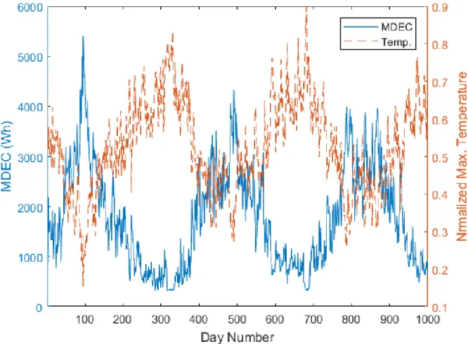
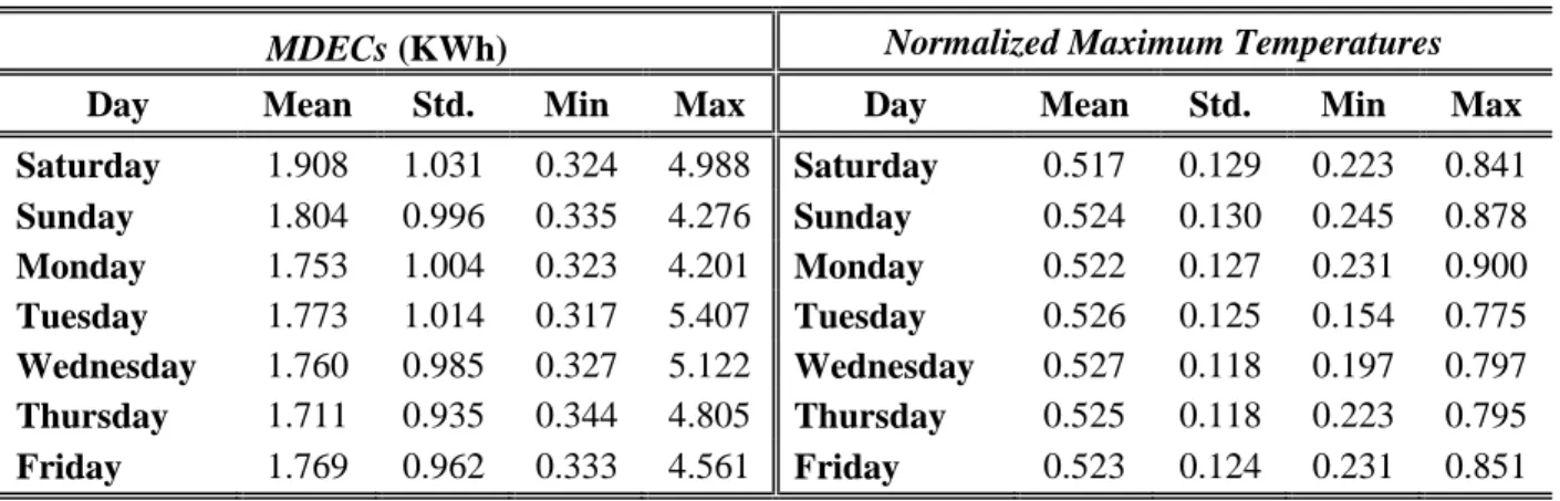
Since our target in this paper is day-ahead forecasting of energy consumption, it is reasonable to utilize energy consumption observations of the previous days and transformed temperature variations as explanatory variables. The descriptor statistics of energy consumption throughout the week are summarized in Table 2. Also, Figure 4 provides a comprehensive view of the nature of the daily variations in energy consumption and temperature variations. The figure shows negative correlation between daily energy consumptions and scaled temperatures. While seasonality is not explicitly treated in the learning framework, it is expected to be captured in the increased MDEC and decreased temperature observations

21 which will describe the projected MDEC estimates. Hence, no data split, for further hierarchy in building additional models that account for seasonality, is required.

Table 2: Descriptive statistics of the case study variables.

MDECs (KWh) Normalized Maximum Temperatures Day Mean Std. Min Max Day Mean Std. Min Max Saturday 1.908 1.031 0.324 4.988 Saturday 0.517 0.129 0.223 0.841 Sunday 1.804 0.996 0.335 4.276 Sunday 0.524 0.130 0.245 0.878 Monday 1.753 1.004 0.323 4.201 Monday 0.522 0.127 0.231 0.900 Tuesday 1.773 1.014 0.317 5.407 Tuesday 0.526 0.125 0.154 0.775 Wednesday 1.760 0.985 0.327 5.122 Wednesday 0.527 0.118 0.197 0.797 Thursday 1.711 0.935 0.344 4.805 Thursday 0.525 0.118 0.223 0.795 Friday 1.769 0.962 0.333 4.561 Friday 0.523 0.124 0.231 0.851

In this work, a fixed input-variable configuration is selected. It is worth mentioning that the specific number of features to be used comprises a different study (feature selection) for ensemble learning frameworks and is beyond the scope of this paper. However, the used feature configuration aligns with that commonly applied in the literature and is justified due to the immediate relation between the target variable and the used features, i.e. explanatory variables [38, 81]. For a given day, the MDEC is assumed to be explained by 8 variables, two temperature variables and six MDEC variables. The temperature variables (represented as the current and day-before maximum linearly-scaled temperatures) are those for the day on which MDEC prediction is considered, and the day before. The six MDEC variables are as follows; the MDEC values of four previous days as well as the MDEC value of the same day, but from two previous weeks. Hence, the six variables have different lags. For example, the ensemble model dedicated to predict the MDEC of a given Saturday will have the input variables as the temperature on the same day, the temperature from the previous Friday, the MDECs from the previous Tuesday to Friday, and the MDECs of two previous Saturdays. Moreover, it is expected that energy profiles, on an individual level, may depend on socio-economic variables. Examples of such variables are the socio-economic state of the country where the household is located, the urban/suburban categorization of the household, changes in household income, etc. On the other hand, it is expected that such variables categorize or scale the expected usage profile among the

22 different households on a long-term basis. Therefore, since the modeling problem is on the household level and in a short-term setting, the economic impact on the targeted energy consumption trends may not be apparent.

Parameter Selection and Model Comparison

The two-stage resampling ANN ensemble framework with robust linear combiner is proposed to predict day-ahead household energy consumption. The search process for the optimum uniform ANN configuration, diversity (or information mixture) parameter and combiner-information parameter are presented here. The information mixture parameter, me, is used to investigate and eventually tune the

information diversity between the ensemble members. The combiner-information parameter, mc, is used to

identify sensitivity and performance of linear combiners to available information for ANN training as well as dedicated information to the combiner’s training. The optimum values of these parameters, along with the ANN sub-models’ parameters, are found by cross-validation studies. Seven ensemble models should be selected to represent each day of the week, as the study will predict day-ahead MDECs for Saturday through Friday. Hence, for each ensemble model, a cross-validation study should be carried out.

Initially, the system inputs and outputs are pre-processed. The observations are normalized and then linearly scaled to meet the range-requirement of the ANN and ensemble members [34]. As described in the methodology, MLP-based feed-forward ANN models are used as the sub-ensembles. All the ANNs will be initiated with one hidden layer because the nature of the input variables does not require further hidden layers. The hidden neurons are defined to utilize log-sigmoid transfer functions. The optimum model configuration of the ANNs, in terms of the number of hidden neurons in the hidden layer, is found via a separate validation study. The number of hidden neurons, which appears to be suitable for all or most of the days, is then selected for all ensemble models. This allows for practically uniform and, therefore, fast application to such case study. Complex-enough ANNs are needed so that overfitting is achieved and the diversity within the ensemble is manifested. Moreover, the validation study is carried out such that 40% of

23 the data is randomly selected and used to train a single model, while the remaining 60% of the data is estimated to evaluate the testing performance. This process is repeated ten times for each hidden neuron configuration and each day of the week. The performance of the ten versions of the same configuration is then averaged to reliably select the best configuration over all the examined ensemble models. A step-by-step summary of the ANN selection study is provided as follows:

1) Retrieve the dataset for a given day of the week.

2) Using random sampling without replacement, split the dataset into testing set and training set, where the testing set comprises 40% of the dataset and the training set has the remainder 60% of the dataset.

3) Initiate the predefined ANN models, each with different number of hidden neurons. 4) Perform training and testing using the constructed training/testing set.

5) Repeat steps 2 to 4 for ten times, where the testing performance for each ANN model is saved after each time.

6) Retrieve the average testing performance of the ANN models and select the ANN configuration with the best performance to represent that day (selected in step 1).

7) Repeat steps 1 to 6 and retrieve the best ANN configuration results for each day of the week. 8) Using majority voting, select the ANN configuration that persists throughout most of the days to

set a uniform-optimal configuration for the ensemble learning framework.

The above procedure indicates that once the optimum ANN configuration for each day is selected, the number of hidden neurons is found as a majority vote and becomes fixed for all the ensemble model validation studies. This will enforce a homogeneous ensemble model (the ANN individual members have the same structure), which will then undergo performance evaluation for each me and mc case. In other

words, the next step is to find the optimum ensemble model, in terms of mixture ratios. To do so, the two-stage resampling is carried out for a different information-mixture me case, after reserving the dedicated

data for combiner training via the mc parameter. At this point, the parallel nature of the ensemble framework

will allow for each sub-ensemble model to be trained in the same time, and the trained ensemble combiner is used to produce the ensemble estimates for that particular ensemble architecture. This process is repeated until the optimum ensemble parameters are found.

24 A Jackknife validation technique is used to evaluate the relative performances of the proposed ensemble models [82]. For a given ensemble model, the Jackknife validation is used to determine the optimum values of me and mc as follows. The MDEC value of an observation is temporarily removed from the database and

is considered as a testing observation. The ensemble members and the ensemble combiners are trained using the data of the remaining observations. Then, sub-ensemble estimates are obtained for the testing observation using the calibrated ensemble model. Figure 5 depicts the process of creating the ensemble learner for any given day. The performance of the proposed model is examined for all the seven days of the week, where each day will have an ensemble model. Jackknife validation is used for each simulation. These simulations investigate different combinations of homogeneity parameters to find the optimum ensemble configuration. In the next section, the validation results are then presented and the performances of the optimal ensemble models are compared to the benchmark studies. The following is a step-by-step summary of the study experiment:

1) Choose a potential ensemble configuration (type and size of ensemble members, k, me, mc, and

ensemble combiner) as described above in this section;

2) Keep one observation from the original sample as a test observation;

3) Create k subsets using the proposed resampling technique and train the ensemble models (members and combiner) using the generated resamples;

4) Estimate the test observation (create the ensemble estimate); 5) Repeat steps 2 to 4 for all observations in a jackknife framework; 6) Repeat steps 1 to 5 for every ensemble configuration;

25 Figure 5: The utilized ensemble learning process, where the different components used in the initial modeling problem

and in the update/forecasting setting are highlighted.

Evaluation Criteria

For each ensemble configuration (in terms of me and mc values), a Jackknife validation is carried out. In

each simulation, the Jackknife process is repeated until we obtain the ensemble estimates for all available observations. The estimates are then evaluated using predefined evaluation criteria in order to select the optimum values for these ensemble parameters. The reason behind using Jackknife validation in this work is due to its ability to evaluate the optimum parameters with relatively better independence of the model’s performance from the available training information [83, 84]. Hence, the final models’ performance for the seven days are presented as jackknife validation results, for the chosen models.

Root mean square error (RMSE), bias (Bias), relative root mean square error (rRMSE) relative bias (rBias) and mean absolute percentage error (MAPE) are used as measures of model performance and generalization ability over different ensemble parameter values, i.e. mixture ratios. The rBias and rRMSE measures are

26 obtained by normalizing the error magnitude of each point by its own magnitude. The MAPE measure is similar to rRMSE and rBias in the relative sense, yet it provides a different outlook on the model’s generalization ability. The considered performance criteria are defined as follows:

𝑅𝑀𝑆𝐸_𝑑= √1 𝑁 ∑(𝑀𝐷𝐸𝐶𝑑𝑖− 𝑀𝐷̂𝐸𝐶𝑑𝑖) 2 𝑁 𝑖=1 (9) 𝑟𝑅𝑀𝑆𝐸𝑑= 100 × √ 1 𝑁 ∑ ( 𝑀𝐷𝐸𝐶_𝑑𝑖− 𝑀𝐷̂𝐸𝐶_𝑑𝑖 𝑀𝐷𝐸𝐶_𝑑𝑖 ) 2 𝑁 𝑖=1 (10) 𝐵𝑖𝑎𝑠_𝑑= 1 𝑁× ∑(𝑀𝐷𝐸𝐶𝑑𝑖− 𝑀𝐷̂𝐸𝐶𝑑𝑖) 𝑁 𝑖=1 (11) 𝑟𝐵𝑖𝑎𝑠_𝑑=100 𝑁 × ∑ ( 𝑀𝐷𝐸𝐶_𝑑𝑖− 𝑀𝐷̂𝐸𝐶_𝑑𝑖 𝑀𝐷𝐸𝐶_𝑑𝑖 ) 𝑁 𝑖=1 (12) 𝑀𝐴𝑃𝐸_𝑑=100 𝑁 × ∑ | 𝑀𝐷𝐸𝐶_𝑑𝑖− 𝑀𝐷̂𝐸𝐶_𝑑𝑖 𝑀𝐷𝐸𝐶_𝑑𝑖 | 𝑁 𝑖=1 (13)

where 𝑀𝐷𝐸𝐶_𝑑𝑖 is the ith observation of the d-day mean daily load (d = Saturday, Sunday, …, Friday), 𝑀𝐷̂𝐸𝐶_𝑑𝑖 is the ensemble model-based estimation of 𝑀𝐷𝐸𝐶_𝑑𝑖, and N is the number of observations.

The use of the above criteria is motivated due to the different information they provide. RMSE and Bias criteria are typical performance measurements. MAPE is a common relative evaluation criterion among energy forecasting studies. However, using this criterion as the only relative measure of error to compare the performance of different methods is not recommended. MAPE may favor models which consistently produce underestimated forecasts. Consequently, rRMSE and rBias complement the latter, as they provide information of the models’ performance distribution. Low rRMSE and rBias values indicate that the target

27 variable’s lower observations have relatively low prediction errors, which is obviously the preferred target. In contrast, if these measures are found high, it would imply that the low and high target variable’s observations are poorly predicted. Hence, using the five error measurement criteria is important.

5. Results and Discussion

Baseline Study

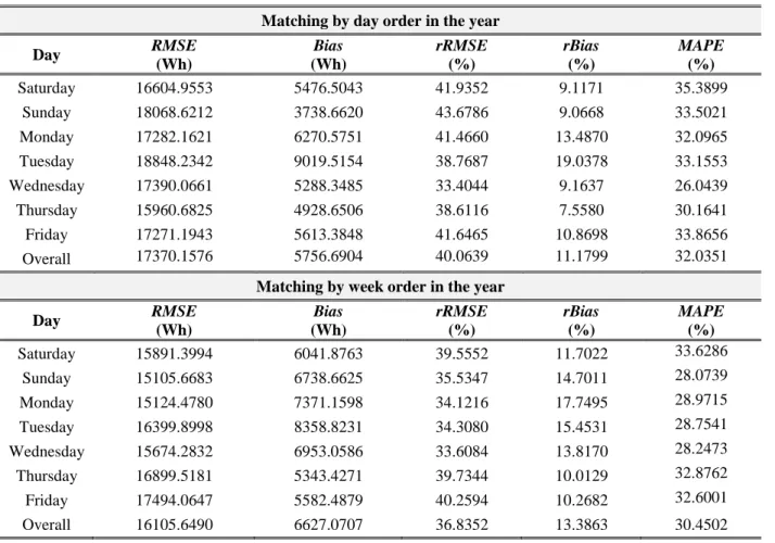
The forecasting error of a baseline model is shown in Table 3 for all days of the week. A baseline model simply takes the previous year’s consumption as the predicted value. This methodology has been utilized in previous work as well as in real-life by utility companies to contextualize model performance [36, 85, 86]. As for the baseline study, the household’s daily energy consumption observations of the year 1997 are used to predict the next year’s daily energy consumption. Furthermore, two procedures are used for the latter in order to provide better investigation; in the first procedure, the days are matched by their order in the year without initial matching of their order in the week. For example, the first day in year 1998 is matched with the first day in year 1997, and then its order in the week is identified. Following on the same example, after matching the first day in 1998 with its predecessor, we note that it is a Tuesday. Finally, the prediction errors for this method are computed. The first procedure allows for all the days in the year to be matched without sacrificing incomplete weeks in the year.

In the second procedure, the weeks are matched by their order in the year. For example, the first complete week in the year 1998 is matched by the first complete week in 1997; this process is continued until all the weeks in the test year are matched by their predecessors. By using this procedure, all the days in the week are automatically matched by their predecessors in the previous year and a direct computation of the prediction errors can be performed. When using this procedure, the first and last incomplete weeks are removed to facilitate the baseline’s matching process.

28 It is clear that such approach produces highly biased estimates and imposes large errors. The errors are not only very high, but also as large as the MDEC Summer values. This observation confirms that relying on such approach, while accepted for aggregated energy consumption profiles, does not provide reliable estimates for individual energy consumption patterns. This can be justified by “the law of large number,” where after a certain aggregation size, an individual pattern does not significantly affect the aggregated pattern of interest [36]. Moreover, at smaller aggregation levels, it is shown that predicting individual consumption patterns produce better generalization than predicting the aggregate profile [16]. As a consequence, in decentralized energy systems, forecasting individual energy consumption and using relatively complex modeling methods is essential.

Table 3: Results from the baseline approach utilizing two different matching procedures. Matching by day order in the year

Day RMSE (Wh) Bias (Wh) rRMSE (%) rBias (%) MAPE (%) Saturday 16604.9553 5476.5043 41.9352 9.1171 35.3899 Sunday 18068.6212 3738.6620 43.6786 9.0668 33.5021 Monday 17282.1621 6270.5751 41.4660 13.4870 32.0965 Tuesday 18848.2342 9019.5154 38.7687 19.0378 33.1553 Wednesday 17390.0661 5288.3485 33.4044 9.1637 26.0439 Thursday 15960.6825 4928.6506 38.6116 7.5580 30.1641 Friday 17271.1943 5613.3848 41.6465 10.8698 33.8656 Overall 17370.1576 5756.6904 40.0639 11.1799 32.0351

Matching by week order in the year

Day RMSE (Wh) Bias (Wh) rRMSE (%) rBias (%) MAPE (%) Saturday 15891.3994 6041.8763 39.5552 11.7022 33.6286 Sunday 15105.6683 6738.6625 35.5347 14.7011 28.0739 Monday 15124.4780 7371.1598 34.1216 17.7495 28.9715 Tuesday 16399.8998 8358.8231 34.3080 15.4531 28.7541 Wednesday 15674.2832 6953.0586 33.6084 13.8170 28.2473 Thursday 16899.5181 5343.4271 39.7344 10.0129 32.8762 Friday 17494.0647 5582.4879 40.2594 10.2682 32.6001 Overall 16105.6490 6627.0707 36.8352 13.3863 30.4502

29 Proposed Ensemble Performance

The proposed robust ensemble framework is demonstrated in the day-ahead forecasting of individual household energy consumption and compared against single models and Bagging models, as described in Section 4. For each day of the week, the models are created and trained. The optimum ensemble parameters for each robust ensemble model are then found using Jackknife simulations over different configurations. Moreover, from the separate validation study, dedicated for selecting the uniform ANN configuration, the optimum configuration of the ensemble members is found such that individual ANNs comprise 1 hidden layer and 16 hidden neurons. However, ANNs are inherently instable learners and they provide different optimum configurations every time a single-model validation study is carried out. Hence, the ensemble of ANNs prompts the important benefit of shifting this validation issue towards the ensemble parameters. In other words, the ensemble model produces enhanced generalization ability, and reduces the dependency of performance stability on the ANN sub-models’ individual generalization ability [58, 87]. In the current study, tackling this problem is important because individual household energy consumption is a relatively complex time series, which induces bigger challenges to single ANNs [88]. This is verified in the results provided in this section.

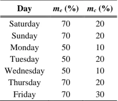
The proposed robust ensemble framework, EANN, is applied on the case study and compared against a single ANN model, SANN, and an ANN-based Bagging ensemble model, BANN. Table 4 shows the results of the optimum EANN configuration for each day of the week. The results agree with the expected behavior as working days, except for Friday. The results show that the household’s MDECs exhibit a more predictable consumption behavior. In addition, the relatively limited mixture of information required by working days suggests that the robust combiners need small amount of information, dedicated for their training. The opposite is seen when the diversity is lowered (higher information sharing), as mc increases

30 This finding further extends the novelty in the proposed ensemble learning framework, as it validates the ensemble learning identity of the proposed method; ensemble learners with higher me are expected to be

coupled with combiners which are trained with higher mc. From Table 4, it can be deduced that the ensemble

model describing Wednesday is found to be the “least complex day”, while Friday is found to be the most complex day. From a household energy consumption viewpoint, the results indicate that the household have fairly regular energy consumption patterns during most of the business days and the proposed model can successfully capture them in the optimum ensemble configuration. On the other hand, energy consumption in Fridays is less regular because the household is expected to consume energy more actively at the end of this business day. Similarly, the proposed ensemble model is able to inform this requirement by the relatively higher information-mixture values for the optimum ensemble model at that day.

Table 4: Ensemble parameters selection.

Day me (%) mc (%) Saturday 70 20 Sunday 70 20 Monday 50 10 Tuesday 50 20 Wednesday 50 10 Thursday 70 20 Friday 70 30

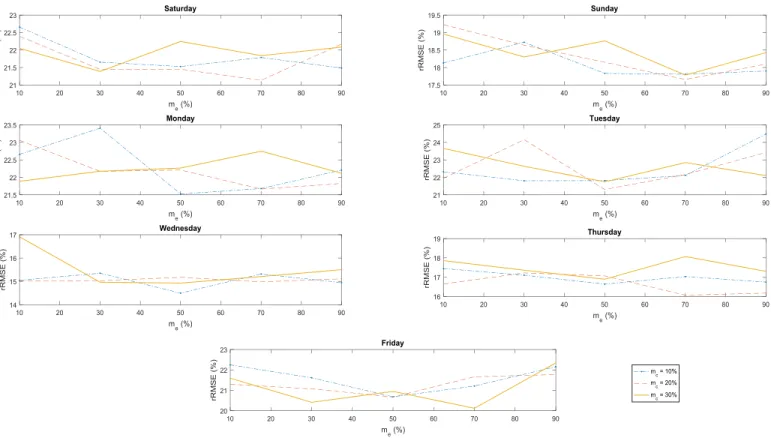
Figure 6 presents Jackknife results for the EANN models’ parameters, performed for each day of the week. Different ensemble configurations are investigated. The figure shows the Jackknife validation performance with respect to changes in the homogeneity parameters. All EANN models provide the best model performance with mixture level values less than unity. This result agrees with the ensemble learning theory and clearly indicates that diversity-controlled ensembles are better than data-saturated ones. In other words, the ensembles do not require all the available training information in order to improve their generalization ability, but rather diverse-enough models with limited information-sharing among their sub-ensembles. In the proposed model, this identity stems from a controlled information-exchange environment suited to the nature of the relationship and the available intelligence on the system. In addition, each curve in Figure 6

31 has a relatively convex shape; this observation suggests that optimal mixture levels are expected to be found between 0 and 1. Each case study is expected to have information-mixture parameter curves with global optimum corresponding to a unique ensemble configuration.

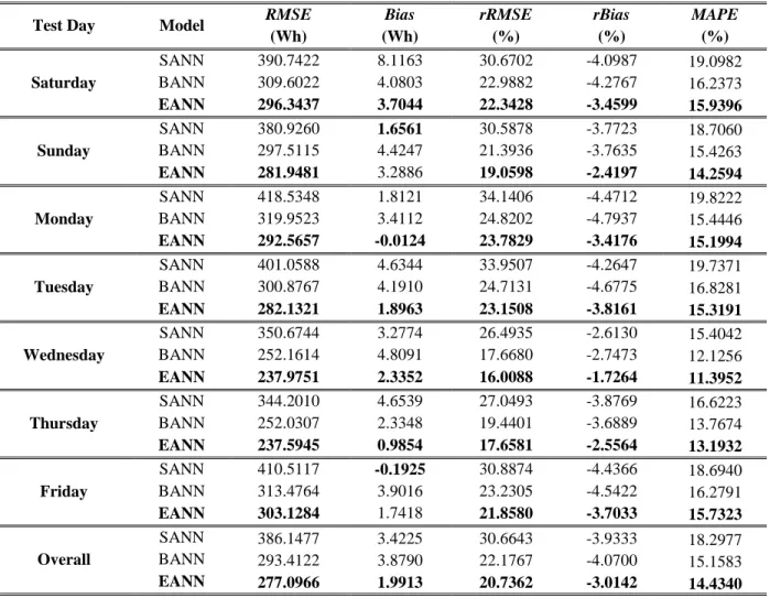
After identifying the best EANN models, summarized in Table 4, their performances are compared to SANN and BANN models. For reliability, all the optimum models are constructed repeatedly, where in each time they are retrained and retested; the average performance is reported. Table 5 presents the performance results of the proposed ensemble, compared to SANN and BANN models. The proposed model has significantly improved the estimation performance in terms of absolute and relative errors. Considering RMSE, rRMSE, and MAPE, the EANN models outperform the SANN and BANN models. BANN models’ performance is slightly better than SANN models’ performance, which is expected from

32 an ensemble model. Among all the day-wise EANN models, EANN models for Wednesday and Thursday have the lowest errors, while EANN model for Friday has the highest error in terms of RMSE, rRMSE, and MAPE results. This important finding further validates the proposed ensemble learning framework’s interpretability. Also, the three measurement criteria have consistent results among themselves throughout the day-wise models. Where the best MAPE result is found (Wednesday), the second-best RMSE (with a close margin from the lowest) and the best rRMSE are also located.

If we recall the results retrieved for optimum day-wise EANN models’ information-mixture parameters, i.e. diversity requirement, the generalization ability is found to be proportional to the amount of information-sharing. For example, the optimum EANN model configuration for Wednesday requires the lowest amount of information-mixture (highest induced diversity) and produces the second-lowest error (second-highest accuracy). In a similar manner, the optimum EANN model configuration for Friday requires the highest amount of information-mixture and has the highest error (lowest accuracy) among all EANN models. It should be noted that most of the day-wise EANN models exhibit this characteristic, except in the EANN model that forecasts Mondays. Due to the heuristic nature of the model, this slight inconsistency is expected. Hence, the novel characteristic of the proposed ensemble framework relates the model’s optimum parameters to its performance and the corresponding physical interpretation of the results is still apparent.

The Bagging ensemble produces inferior results in terms of Bias and rBias criteria, even when compared to the SANN models. EANN also outperforms BANN in terms of Bias in all the days, with 5 out of 7 days when compared to SANN models. The EANN clearly outperforms SANN and BANN in rBias and provides the biggest improvement in this error criterion. The significant improvement by EANN in rBias is also a positive feedback on the proposed ensemble since most of the relevant studies in the literature use similar criterion to evaluate the model performance. To this extent, the poor BANN performance in the Bias and rBias criteria exemplifies one of the main limitations discussed regarding the common ensemble learners, which is partly due to their relatively simple ensemble integration methods; the utilization of the diverse

33 ensemble model with the robust linear combiner significantly reduces the Bias errors among all the EANNs. This result confirms the added benefit from utilizing the proposed ensemble learning framework. In the current study, the bias in estimates is expected to persist due to the various challenges inherent in forecasting the individual household energy consumption time series, as discussed in Section 2. Hence, the robust combiner of the proposed ensemble framework overcomes such challenges as opposed to the conventional ensemble models.

Furthermore, the overall performance of the three models is shown at the end of Table 5. This performance is computed when the forecasts coming from all the day-wise models are combined in one dataset and then compared to their corresponding true observations. The overall performance by the EANNs is the best among all the five error measurement criteria, where the relative improvement of EANN (compared with SANN and BANN) is 6% to 28% in RMSE, 42% to 49 in Bias, 7% to 32% in rRMSE, 23% to 26% in rBias, and 5% to 21% in MAPE. The overall performance results further verify the significant improvement which the proposed ensemble learning framework can bring to short-term forecasting of individual household energy consumption.

It is worth noting that seasonality, whether in climate patterns or in energy consumption patterns throughout the year, is not expected to be a significant contributor to the uncertainty in short-term energy forecasts, as described in Section 4. However, the representativeness of the dataset may have implications on the heuristic performance. On one hand, this may relieve the learner from comprehending various consumption patterns throughout the year and fit more concisely on what the cluster pertains. On the other hand, in the case of limited dataset, such hierarchy or clustering approach to data may result in inferior performance due to the threshold of available intelligence in each cluster [27, 34]. Investigating the effects of various feature selection and preprocessing frameworks are usually considered a whole research endeavour, at least in the pure literature (machine learning literature). Hence, the scope of the current paper is defined to utilize useful features which are in-line with the expected behaviour of the household energy consumption for each day of the week. Furthermore, preprocessing the dataset to comprise subsets with pre-informed consumption

34 patterns may influence the proposed ensemble performance, and all other models, in a similar fashion. Consequently, the proposed ensemble model as well as the other models are expected to yield performances relative to that in the current work, in the case of utilizing different feature selection and preprocessing approaches.

Table 5: Average performance results of the Jackknife validation trials for each SANN, BANN and EANN models.

Test Day Model RMSE (Wh) Bias (Wh) rRMSE (%) rBias (%) MAPE (%) Saturday SANN 390.7422 8.1163 30.6702 -4.0987 19.0982 BANN 309.6022 4.0803 22.9882 -4.2767 16.2373 EANN 296.3437 3.7044 22.3428 -3.4599 15.9396 Sunday SANN 380.9260 1.6561 30.5878 -3.7723 18.7060 BANN 297.5115 4.4247 21.3936 -3.7635 15.4263 EANN 281.9481 3.2886 19.0598 -2.4197 14.2594 Monday SANN 418.5348 1.8121 34.1406 -4.4712 19.8222 BANN 319.9523 3.4112 24.8202 -4.7937 15.4446 EANN 292.5657 -0.0124 23.7829 -3.4176 15.1994 Tuesday SANN 401.0588 4.6344 33.9507 -4.2647 19.7371 BANN 300.8767 4.1910 24.7131 -4.6775 16.8281 EANN 282.1321 1.8963 23.1508 -3.8161 15.3191 Wednesday SANN 350.6744 3.2774 26.4935 -2.6130 15.4042 BANN 252.1614 4.8091 17.6680 -2.7473 12.1256 EANN 237.9751 2.3352 16.0088 -1.7264 11.3952 Thursday SANN 344.2010 4.6539 27.0493 -3.8769 16.6223 BANN 252.0307 2.3348 19.4401 -3.6889 13.7674 EANN 237.5945 0.9854 17.6581 -2.5564 13.1932 Friday SANN 410.5117 -0.1925 30.8874 -4.4366 18.6940 BANN 313.4764 3.9016 23.2305 -4.5422 16.2791 EANN 303.1284 1.7418 21.8580 -3.7033 15.7323 Overall SANN 386.1477 3.4225 30.6643 -3.9333 18.2977 BANN 293.4122 3.8790 22.1767 -4.0700 15.1583 EANN 277.0966 1.9913 20.7362 -3.0142 14.4340 Bold numbers indicate best results

At this point, the expected performance of the proposed model has been investigated over the five considered error measurement criteria; to provide a complete assessment on the stability of the proposed ensemble, the variation of the proposed model’s performance criteria from their expected values should also be investigated. Due to the nature of the forecasting problem, the stability of the relative performance measurement criteria is considered, rRMSE, rBias, and MAPE criteria. Moreover, the variation results can