HAL Id: hal-01247882
https://hal.archives-ouvertes.fr/hal-01247882
Submitted on 22 Dec 2015
HAL is a multi-disciplinary open access
archive for the deposit and dissemination of
sci-entific research documents, whether they are
pub-lished or not. The documents may come from
teaching and research institutions in France or
abroad, or from public or private research centers.
L’archive ouverte pluridisciplinaire HAL, est
destinée au dépôt et à la diffusion de documents
scientifiques de niveau recherche, publiés ou non,
émanant des établissements d’enseignement et de
recherche français ou étrangers, des laboratoires
publics ou privés.
Niño Southern Oscillation patterns
Iván Cárdenas-Gallo, Raha Akhavan-Tabatabaei, Mauricio Sánchez-Silva,
Emilio Bastidas-Arteaga
To cite this version:
Iván Cárdenas-Gallo, Raha Akhavan-Tabatabaei, Mauricio Sánchez-Silva, Emilio Bastidas-Arteaga.
A Markov regime-switching framework to forecast El Niño Southern Oscillation patterns. Natural
Hazards, Springer Verlag, 2016, In press, 81 (2), pp.829-843. �10.1007/s11069-015-2106-y�.
�hal-01247882�
Natural Hazards manuscript No. (will be inserted by the editor)
A Markov regime-switching framework to forecast El Ni˜no
Southern Oscillation patterns
Iv´an C´ardenas-Gallo · Raha Akhavan -Tabatabaei · Mauricio S´anchez-Silva · Emilio Bastidas-Arteaga
Received: 26 March 2015 / Accepted: 30 November 2015
Abstract The El Ni˜no-Southern Oscillation (ENSO) is an ocean-atmosphere phenomenon involving sustained sea surface temperature fluctuations in the Pacific Ocean, causing dis-ruptions in the behavior of the ocean and atmosphere. We develop a Markov switching au-toregressive model to describe the Southern Oscillation Index (SOI), a variable that explains ENSO, using two autoregressive processes to describe the time evolution of SOI, each of which associated with a specific phase of ENSO. The switching between these two models is governed by a discrete time Markov chain (DTMC), with time-varying transition proba-bilities. Then, we extend the model using sinusoidal functions to forecast future values of SOI. The results can be used as a decision-making tool in the process of risk mitigation against weather and climate related disasters.
Keywords ENSO · Markov-Switching · Autoregressive processes · Forecasting · Regimes
1 Introduction
The El Ni˜no-Southern Oscillation (ENSO) is an ocean-atmosphere event that involves sus-tained sea surface temperature fluctuations in the Pacific Ocean. This causes a disruption in the behavior of the ocean and the atmosphere, having important consequences for the global weather (National Oceanic and Atmospheric Administration, 2010). This phenomenon is I. C´ardenas
Centro para la Optimizaci´on y la Probabilidad Aplicada (COPA), Departamento de Ingenier´ıa Industrial, Uni-versidad de los Andes, Bogot´a, DC, Colombia, E-mail: [email protected]
R. Akhavan-Tabatabaei (corresponding author)
Centro para la Optimizaci´on y la Probabilidad Aplicada (COPA), Departamento de Ingenier´ıa Industrial, Uni-versidad de los Andes, Bogot´a, DC, Colombia, E-mail: [email protected]
M. S´anchez-Silva
Risk and Reliability in Civil Engineering, Departamento de Ingenier´ıa Civil, Universidad de los Andes, Bo-got´a, DC, Colombia, E-mail: [email protected]
E. Bastidas-Arteaga
LUNAM Universit´e, Universit´e de Nantes-Ecole Centrale Nantes, GeM, Institute for Research in Civil and Mechanical Engineering/Sea and Littoral Research Institute, CNRS UMR 6183/FR 3473, Nantes, France, E-mail: [email protected]
Cárdenas-Gallo I, Akhavan-Tabatabaei R, Sanchez-Silva M, Bastidas-Arteaga E (2016). A Markov regime-switching framework to forecast El Niño Southern Oscillation patterns. Natural Hazards. In press. http://doi.org/10.1007/s11069-015-2106-y
not completely predictable because of the complexity that results from the relationships between ocean currents, atmospheric circulation and winds in the Pacific. ENSO involves two cyclic phases; El Ni˜no and La Ni˜na. El Ni˜no represents the warm phase of the ENSO. During this phase, the sea surface temperatures rise along the North-West coast of tropical South America. The impacts of El Ni˜no episodes depend on the geographical location. For example, in Colombia El Ni˜no results in long periods of droughts leading to problems in the agriculture sector, hydroelectric generation and water supply for vulnerable populations. El Ni˜no is only one phase of the phenomenon. An episode of La Ni˜na is followed most of the times by the El Ni˜no episode. La Ni˜na represents the cool phase of the ENSO and is associated with the cooling of ocean waters of the coast of Peru and Ecuador. Its impacts are completely opposite to those of El Ni˜no. During La Ni˜na conditions in Colombia, the amount of precipitations increases leading to floods, landslides and damages to civil infras-tructure.
The importance of the phenomenon lies in its effect on the global climate. Although ENSO events are characterized by a fluctuation in ocean temperatures in the equatorial Pa-cific, they are also associated with changes in wind, pressure, and rainfall patterns. This set of climate changes cause a significant impact across the tropical Pacific region and areas away from it. Many studies have found a close relationship between Pacific sea surface tem-perature (SST) anomalies and precipitation (Li,2013). As mentioned above, during El Ni˜no and La Ni˜na the usual precipitation patterns can be greatly disrupted by either excessively wet or dry conditions (International Research Institute for Climate and Society, 2008) that may impact the global weather. Therefore, the ability to forecast El Ni˜no and La Ni˜na events is extremely important to define risk mitigation measures.
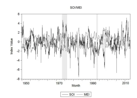
There are several indicators that provide information about the state of ENSO at a given time. One of them is the Southern Oscillation Index (SOI), which is calculated from the monthly fluctuations in the air pressure difference between Tahiti and Darwin. Sustained negative values of the SOI indicate El Ni˜no episodes, while sustained positive values of the SOI indicate La Ni˜na episodes. Another indicator of ENSO is the Multivariate ENSO Index (MEI), which is a monthly measure based on the six main observed variables over the tropical Pacific. MEI contains information of the sea level pressure, surface wind (East-West and North-South), sea surface temperature, surface air temperature and total cloudiness of the sky. In this case, sustained negative values of the MEI indicate La Ni˜na episodes, and sustained positive values of the MEI indicate El Ni˜no episodes. In Figure 1, we can observe the SOI and MEI from 1950 to 2012. Moreover, in Figure 1 it is possible to observe the two strong episodes of ENSO in the shaded areas: one El Nio episode from July-1993 to December-1993, and one La Nia episode from June-1973 to March-1976.
Poveda et al.(2010) reviewed the hydro-climatic variability of the Colombian Andes associated with El Ni˜no-Southern Oscillation (ENSO) using records of rainfall, river dis-charges, soil moisture and a vegetation index (NDVI). Their conclusions point to define ENSO as the main forcing mechanism of interannual climate variability. Given the indexes that were described previously (SOI and MEI), they quantify the anomalies in the sea sur-face temperature in terms of their sign, timing and magnitude. These studies indicate that ENSO indexes become important and valuable tools to forecast several hydro-climatological variables in the region.
Over time, several models have been developed to forecast the behavior of the phe-nomenon. This effort has resulted in the atmospheric general circulation models (AGCMs). AGCMs of the atmosphere, ocean and sea ice were coupled and run asynchronously to pro-duce credible simulations of the global climate (Meehl,1990). Given the implicit complexity to model the weather physically, this kind of approach becomes accessible only for national
Fig. 1 Evolution of the index SOI and MEI over time (1950-2012).
institutions that have the technology and equipment needed. Another alternative that has been used to forecast the behavior of the phenomenon is the application of statistical models as the proposed in Ubilava et al. (2013) and Zhou et al.(2009). Ubilava et al.(2013) present a smooth transition autoregressive (STAR) modelling framework to assess the potentially smooth regime-dependent dynamics of the sea surface temperature anomaly. On the other hand, Zhou et al. (2009) emphasized on the assimilation of historic SST (Sea Surface Tem-perature) data to improve ENSO hindcasts. Thus, predictions are based on the behavior of climatic variables during the last years. These approaches aim to identify correlations in order to establish patterns in the behavior of the relevant variables.
Most statistical models that have been developed for climatic variables are based on the Box-Jenkins methodology (BoxJenkins,1976). These models can represent the basic structure of the time series, but they fail to reproduce the nonstationary behavior that exists in climatic variables. A source of non stationarity is the existence of cyclic patterns that determine the behavior of the weather. For example, El Ni˜no-Southern Oscillation (ENSO) is a cyclical process composed of a warm phase (El Ni˜no) and a cool phase (La Ni˜na).
Given the existence of cyclical processes, several models have been developed to include the fact of various changing regimes over time. For example, Ubilava et al. (2013) adopted a smooth transition autoregressive modeling framework to explain the sea surface temperature in order to forecast ENSO; they argued the advantage of nonlinear models to represent dynamic processes such as ENSO. In order to model the weather, the introduction of a variable that represents the weather type (regime) can be seen in Zucchini et al. (2009) where Hidden Markov Models (HMM) are proposed for modeling the space-time evolution of daily rainfall.
HMMs have a variety of application, including the econometric models. Hamilton et al.(1989) proposes econometric time series, which are composed of a Hidden Markov Model (HMM) and autoregressive models. In Markov Switching Autoregressive (MS-AR) models, several autoregressive models are used to describe the time evolution of the series and the
switching between these different models is controlled by a Hidden Markov chain which represents the possible regimes. MS-AR models were extended by Andrew Filardo (Fi-lardo,1994) who incorporated time-varying transition probabilities (TVTP) between regimes. Since its publication, several applications of the model have been implemented. Ailliot et al. (2012) propose a Markov-Switching Autoregressive model to describe the behavior of wind time series obtaining a good fit to the data. Souza et al. (2010) used a Hidden Markov Model (HMM) to predict future crude oil price movements. Their results indicate that the proposed model might be a useful decision support tool. Walid et al. (2011) proposed a Markov Switching model to investigate the exchange rates for four emerging countries over the period 1994-2009. Yuan (2011) presents an exchange rate forecasting model which com-bines the multi-state Markov Switching model with smoothing techniques. Guo et al. (2010) focus on detecting hot and cold IPO (Initial Public Offering) cycles in the Chinese A-share market using a Markov regime switching model. The hot and cold periods and their turning points are detected clearly (A hot period is related to positive market conditions). Fallahi et al. (2014) used Markov Switching models to identify and analyze the cycles in the un-employment rate and four different types of criminal activities in the US. Finally, Liu et al. (2006) developed a Markov regime Switching model with two regimes representing expan-sion and contraction to catch the cyclical behavior of the semiconductor business.
The main objective of this paper is to propose an MS-AR, in order to evaluate the pattern changes of ENSO along the time and to predict its behavior for the next years. This model contributes to the prediction of hydro-climatic variables, with significant practical implica-tions for agriculture, hydropower generation, fluvial transport, natural hazards and disasters, and human health. The paper is organized as follows: Section 2 describes the proposed model analyzing its advantages and shortcomings. Section 3 presents the steps followed for the model implementation. Section 4 summarizes the results obtained showing the adequacy of the model to establish forecasts. Finally, several concluding remarks are given in the last section.
2 The Proposed - Markov Switching Autoregressive Model (MS-AR)
ENSO is a cyclical phenomenon in which it is possible to identify two regimes over time (La Ni˜na and El Ni˜no). The behavior patterns during each of the two phases are opposite and differentiable. On the other hand, the duration and the change between regimes is vari-able over time. Also, there is uncertainty about the length of episodes or phase transitions. This group of characteristics is properly evaluated by the Markov Switching Autoregressive Model (MSAR) proposed by Hamilton (1989) and improved by Filardo (1994). In this sec-tion we present the model, its applicasec-tion and relevant considerasec-tions for its implementasec-tion. Certain variables undergo episodes in which the behavior of the series seem to change quite dramatically according to a set of regimes. A MSAR model proposes a very tractable approach to model changes in regime. In order to develop a model that allows a given vari-able to follow a different time series process over time (yt), consider a first-order
autore-gression in which the constant term c and the autoregressive coefficientf might be different for each regime stproposed:
yt=cst+fstyt 1+et, (1)
whereet⇠ i.i.d N(0,s2). In order to model the change in regime over time we use a Discrete
values according to a state-space {1,2,...,N}. Also, the probability that st+1 equals some
particular value j depends on the past only through the most recent value st:
P{st+1=j | st=i,st 1=k....} = P{st+1=j | st=i} = pi j (2)
The transition probability pi jgives the probability that state i will be followed by state j in a
one-step transition. It is often convenient to collect the transition probabilities in an (N ⇥N) matrix P known as the transition probability matrix.
In this way, a MS-AR process is a discrete-time process with two components {St,Yt}.
For our case, Ytdenotes the monthly index of SOI with values in ( •,•) and St2 {Ni˜no(1),
Ni˜na(2)} represents the regime at month t. Then, the MS-AR process is characterized by the following two conditional independence assumptions:
– The conditional distribution of Stgiven the values of {St0}t0<tand {Yt0}t0<tonly depends
on the value of St 1. In this manner, we assume that the weather type Stis a first order
Discrete Time Markov Chain.
– The conditional distribution of Ytgiven the values of {St0}t0<tand {Yt0}t0<tonly depends
on the value of St and Yt 1, ...,Yt p. In this manner, we assume that the value of SOI
(Yt)is an autoregressive process of order p whose coefficients evolve in time according
to the regime St.
Hamilton (1989) assumes Fixed Transition Probabilities (FTP) for the DTMC. The as-sumption that the transition probabilities are time-invariant implies that the expected dura-tions of phases do not vary over time. Due to the variability of the ENSO, this assumption might be too strong. El Ni˜no occurs irregularly, with a recurrence ranging from two to eight years with variation in intensity. Each episode lasts about six to fifteen months. On the other hand, La Ni˜na occurs less frequently than El Ni˜no, and an episode lasts from nine months to three years. Therefore, we implemented a Markov-Switching estimation procedure that incorporates time-varying transition probabilities (TVTP) into the Discrete Time Markov Chain (Filardo,1994). There are advantages to using the MS-AR (TVTP) against MS-AR (FTP):
– The TVTP model allows the transition probabilities to decrease or increase after a change of regime. In this way, TVTP models have the flexibility to identify systematic variations in the transition probabilities after turning points.
– The TVTP model captures more complex temporal persistence of the phases than an FTP model. Allowing the transition probabilities to change over time can represent long periods of a specific regime.
– The TVTP model permits time varying expected durations of the phases. It represents a strong advantage over FTP, in which the expected durations of phases are constant along the time.
The TVTP Markov-Switching model for the values of SOI, ytis presented below:
yt=µ1+F(L)(yt 1 µSt 1) +et i f state 1 (Ni˜no), (3)
yt=µ2+F(L)(yt 1 µSt 1) +et i f state 2 (Ni˜na), (4)
whereF(L) = f1+f2L + ... +frLr 1 is the lag polynomial, µSt is the state-dependent
mean,et⇠ i.i.d N(0,s2)and St2 {Ni˜no(1),Ni˜na(2)}. The variation from the FTP model
P{St+1=st+1| St=st,zt} =
p
11(zt) 1 p11(zt)
1 p22(zt) p22(zt) , (5)
where zt={zt,zt 1, ...,zt p} is referred to the values of MEI. In consequence, the monthly
index of MEI becomes a support variable in the model. In the following section we present in detail the implementation of the proposed model.
3 Implementation
This section presents the implementation of the ENSO indexes, along with the description of our proposed methodology. First, it is necessary to identify the order of the autoregressive model (p) to capture the dynamic nature of the phenomenon. During this step, the autocor-relation function (ACF) and partial autocorautocor-relation function (PACF) plots permit to identify the number of autoregressive terms that are needed, the estimation of the parameters includ-ing autoregressive coefficients and transition probabilities. Finally, we revise the model in order to determine whether the specified and estimated model is adequate.
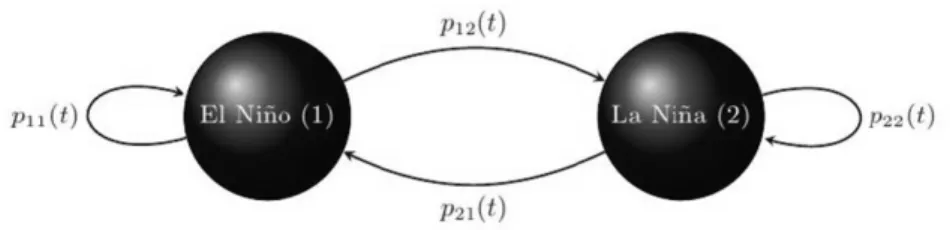
Fig. 2 Transition probability diagram of the DTMC including Time Varying Transition Probabilities. During the MS-AR model specification, the number of regimes and the order p of the autoregressive process were obtained. For our particular model, we defined two regimes trying to represent each phase of the ENSO. In this way, the state space of the Discrete Time Markov Chain is St2 {Ni˜no(1),Ni˜na(2)}. According to our experiments adding a third state
associated with the neutral phase does not improve the results, while adding to the model complexity. The model can be observed in Figure 2. Moreover, the results obtained support the proposal of having only two states. On the other hand, we proposed an autoregressive process of order p = 2 based on the Bayesian Information Criterion (BIC). When choosing from several models, the one with the lowest BIC is preferred. Thus, the autoregressives processes are going to follow this structure:
yt=c1+f11yt 1+f21yt 2+et i f state 1, (6)
yt=c2+f12yt 1+f22yt 2+et i f state 2, (7)
wherefj
i represents the autoregressive coefficient of order i for regime j, cjis the constant
of the process for regime j 2 {Ni˜no(1),Ni˜na(2)}, and et⇠ i.i.dN(0,s2)is a white-noise
For example, the dataset presented in Figure 1 that was used to build the model has a monthly record since 1950 to 2000 and was downloaded from the National Climatic Data Center (NCDC) in Colombia web site (National Climate Data Center, 2013). Given the model specification, the estimation of the autoregressive coefficients and the transition probabilities were developed in the computational software Eviews 8. The software uses the likelihood-based iterative algorithm proposed by Hamilton et al.(1989), whose output is shown in Table 1. As it can be observed in Table 1, each one of the estimated coefficients is statistically significant (Prob. < 0.05). Consequently, the MS-AR(2) model is statistically significant to represent the data series of SOI. The standard errors and the p-values are es-timated by the software EViews 8. The standard errors are computed using the generalized method of moments (GMM) formalized by Hansen (1982). On the other hand, the p-values are obtained via the numerical method proposed by Hansen (1992). Furthermore, the esti-mation of the transition probabilities required in the model was also carried out. Note that the transition probabilities change over time (TVTP); the results are presented in Figure 3.
Variable Coefficient Std. Error z-Statistic Prob. Regime 1 (El Ni˜no)
c1 -1.052 0.192 -5.487 0.000
f1
1 0.428 0.065 6.537 0.000
f1
2 0.199 0.068 2.925 0.003
Regime 2 (La Ni˜na)
c2 0.640 0.165 3.889 0.000
f2
1 0.384 0.066 5.803 0.000
f2
2 0.176 0.065 2.718 0.006
Table 1 MS-AR(2) coefficients
Fig. 3 Evolution of the DTMC Transition Probabilities over time.
As it can be seen in Figure 3, the transition probabilities of being in the same state (p11,p2,2)are approximated to one or zero for various periods. Each of these periods
repre-sent a historical episode of El Ni˜no or la Ni˜na. Thus, during the months in which an episode of El Ni˜no occurred, the probability of remaining in regime 1 (p11)is close to one. On the
other hand, during these time intervals, the probability of remaining in regime 2 (p22)is
close to zero. For example, one historical event of El Ni˜no took place during 1993. For this year, we can clearly observe the related behavior in Figure 3. As it might be expected, the same pattern can be observed during historical episodes of La Ni˜na. A clear example could be the episode of 1975.
In Figure 4, historical episodes of El Ni˜no are shaded in dark grey. During these time intervals, it can be seen that the probability of being in state 1 (El Ni˜no) is approximately one. Likewise, historical episodes of La Ni˜na are shaded in light grey. For these time periods, the probability of being in state 1 (El Ni˜no) is close to zero. Based on these probabilities, we performed a validation process for the model. The duration of each of the episodes based on the model was identified and compared against the historical reports. The results obtained are presented in Table 2. They indicate that the model adequately captures the duration of episodes of both regimes.
Episode Historical Duration Model Duration Regime 1 (El Ni˜no)
March 1951 to February 1952 12 12 March 1957 to November 1957 9 8 September 1963 to March 1964 6 7 March 1965 to November 1965 9 9 June 1969 to February 1970 9 9 March 1972 to December 1972 9 9 June 1977 to November 1977 6 5 April 1982 to February 1983 11 12 May 1987 to January 1988 10 11 July 1993 to December 1993 6 6 March 1994 to December 1994 10 9 April 1997 to March 1998 12 12
Regime 2 (La Ni˜na)
January 1950 to February 1951 14 15 April 1954 to January 1957 34 32 April 1964 to October 1964 7 7 June 1970 to March 1972 22 23 June 1973 to Marc 1976 34 34 April 1988 to July 1989 15 15 Table 2 Comparison between historical and the proposed model durations of ENSO episodes
From the transition probabilities, it is possible to infer the occurrence of El Ni˜no and la Ni˜na episodes. In this way, the MS-AR model allows to make inferences about when the episodes have occurred based on the observed behavior of the series. In Figure 4, the conditional probability of being in state 1 (El Ni˜no) given the two previous observations of yt(P[St=1 | yt,yt 1,yt 2]) is plotted. As we only have two states, the probability of being
in state 2 (La Ni˜na) is computed as the complement probability.
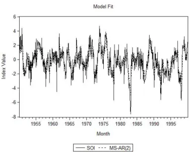
After the estimation of all the parameters of the MS-AR model, we verified its fitting to the data. In Figure 5 the actual values of SOI (1950 2000) are plotted against the values obtained by the proposed MS-AR(2) model. It can be observed that the proposed model captures the behavior of the index over time, highlighting the adequacy of the model. Also, it identifies the peaks and drastic changes in SOI along time. Likewise, it follows the trends
Fig. 4 Conditional probability of being in state 1 (El Ni˜no) given the two previous observations of yt(P[St= 1 | yt,yt 1,yt 2]).
observed during the historical episodes. When values remain positive or negative, the model reproduces the same pattern.
The final stage of the implementation consists of verifying the fit of the model by analysing the residuals. The residuals are defined as the difference between the actual values of SOI and values obtained by the MS-AR(2) model proposed. Both set of values are plotted in Figure 5. The residuals should follow a white-noise process. Thus, it was assessed with statistical tests that the expected value of the residuals is zero. On the other hand, to verify that the residuals are not correlated, the corresponding autocorrelation function (ACF) was developed, and as a result of this we concluded that the residuals are not correlated for any lag. In the following section the implemented model is used to perform forecasts.
4 Forecasting SOI
One objective of this paper is to develop a stochastic model that allows us to predict future values of the SOI index, which is associated with ENSO. The MS-AR(2) model that was implemented in the previous section is useful to describe and analyze the data over time. However, an extension to the model is needed to forecast the SOI index. The main problem is the estimation of the transition probabilities of the Discrete Time Markov Chain. These are completely dependent on the support variable, for our particular application the MEI index. If we want to forecast future values of SOI, it is fundamental to estimate the transition probabilities for those months in the future. In this section we present a method to estimate future transition probabilities.
The proposed approach consists of representing the cyclic seasonality observed in the transition probabilities over time, with a sinusoidal function due to the cyclical behavior of the ENSO phenomenon. Thus, the time series (St) is represented as a periodic function with
period s in which St=St s. The angular frequency w =2ps indicates the angle in radians that
is passed in a unit of time, taking into account that the complete cycle is 2p. To define the length of the period s, we used the expected durations of the El Ni˜no and La Ni˜na episodes. On average, El Ni˜no epidodes last for 6 months, while La Ni˜na epidodes have an average duration of two years. As a result, the length of the period s is established at 28 months. This implies that the transition probabilities p11 t have a cyclical seasonality with s = 28
months. The time series was approximated with the following sinusoidal function.
p11 t=µ + Rsin(wt + q) + at, (8)
whereq is an initial offset angle that permits a more general adjustment to a data set. The constant R represents the amplitude of the cycle. Also, seasonal oscillations occur around the mean value of the seriesµ. Finally, we assume a random error at with mean equal to
zero, constant variance and normal distribution. To fit this model to the data series of p11,
we modify Equation 8 using trigonometric identities:
p11 t=µ + Rsin(wt)sin(q) + Rcos(wt)cos(q) + at. (9)
Now defining A = Rsin(q) and B = Rcos(q), the expression concludes in:
p11 t=µ + bb Asin(wt) + bBcos(wt) + at. (10)
The resulting model is linear with three unknown parameters which can be estimated by least squares. In this way, a sinusoidal function is fit to the monthly time series of the transition probabilities (p11) which is shown in Figure 3.
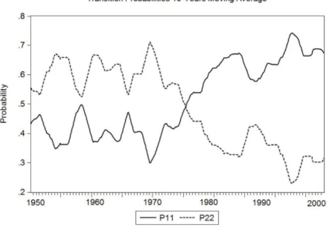
An important contribution in the implementation of the MS-AR(2) model in Section 4 is related to the increase of persistence in time of the El Ni˜no state. Over the years, the probability of being in state 1 (El Ni˜no) seems to augment. To verify this behavior, we performed a 10 year moving average for the transition probabilities (p11and p22). The result
of this procedure is plotted in Figure 6.
Fig. 6 DTMC transition probabilities 10 years moving average.
The increasing trend in the persistence of El Ni˜no state is evident from Figure 6. This conclusion is supported by climatic studies that have been conducted to evaluate the effect of climate change on global phenomena. Results from several earlier global climate model studies indicated that as global temperatures rise due to increased greenhouse gases, the mean pacific climate will tend to resemble an El Ni˜no - like state (Meehl,2000). This fact must be taken into account when estimating the transition probabilities. Consequently, we added the observed trend into the function described in Equation 10. Thus, the final function to estimate the transition probabilities is shown in Equation 14.
p11 t =bµ + bAsin(wt) + bBcos(wt) + btt + at (11)
p11 t =0.5043 0.2081sin(wt) 0.1202cos(wt) + 0.0016t + at (12)
To evaluate the goodness of the predictions, the evaluation period is defined for the months between January 2000 and December 2005. Therefore, the transition probabilities were estimated for these months using the function given in Equation 15. The result of this procedure is shown in Figure 7.
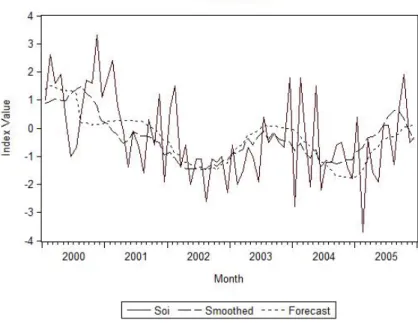
Given the random nature of the Discrete Time Markov Chain, forecasts that are per-formed with the model are random variables. Monte Carlo simulation can be used to evaluate the accuracy of the model. For our particular application, we performed 1000 replications. Then, the monthly average values are computed and presented in Figure 8. The objective of the model is to capture patterns of behavior on the SOI index. The fact of forecasting exact values, peaks and drastic changes is not included in the scope of the model. Therefore, with the aim of properly comparing forecasts with historic values, the historic curve was smoothed with the technique of moving averages. The overall results of the forecast can be
Fig. 7 Estimated DTMC Transition Probabilities using Sinusoidal function.
Fig. 8 Comparison between the forecast obtained with the proposed model and the SOI index (2000-2005). detailed in Figure 8. The error in the forecasts was measured using the mean absolute error (MAE = 0.6254) with respect to the smoothed curve. Moreover, given the random nature of
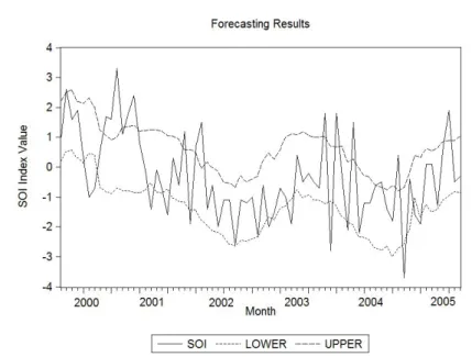
Fig. 9 Comparison between the actual value of SOI the 95% prediction intervals obtained with the proposed model.
the forecasts we computed 95% prediction intervals for each of the months in analysis. In Figure 9 the actual value of SOI and the lower and upper limits for each of the prediction in-tervals are plotted. For 58% of the months, the actual value of SOI was within the prediction interval.
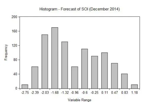
The MS-AR(2) model is able to reproduce the behavior of the smoothed curve. When the index is negative, the average of the forecasts is also negative. This fact also happens in case of positive values. Therefore, it is possible to infer that the model is useful to predict the future behavior patterns of ENSO. The forecast for the next five years (December 2013 - December 2018) has been done and presented in Figure 10. As a result of the forecast done in November 2013, two episodes of El Ni˜no are predicted to occur from September 2014 to June 2015 and July 2017 to January 2018. It should be noted that the predictions were performed with the average of the 1000 simulations. However, from the results it is possible to compute the probability distribution of the forecast in a histogram. For example, the histogram associated with the forecast of SOI for December 2014 is presented in Figure 11. In this way, each monthly forecast may be fit to a known distribution. This fact becomes more useful than obtaining a single value for each month because it is possible to observe the behavior of the forecast over time and calculate the probability that the index variable (SOI) exceeds a particular value. This information is useful to identify the probability of occurrence of extreme events.
5 Concluding remarks
This paper investigates the use of MS-AR model to describe time series associated with ENSO. Our methodology is based on a two regime Markov Switching Autoregressive model that allows separate estimation between El Ni˜no and La Ni˜na episodes. After implementing the model in Section 3 and extending it with a sinusoidal function in Section 4, forecasts
Fig. 10 Forecast obtained with the proposed model for the SOI index (2014-2018).
were performed and compared with historical values. The obtained results indicate that the model fits well to the time series. On the other hand, the forecasts were able to capture the behavior pattern of the index SOI showing the virtues of the model. The proposed model is a very tractable approach to modeling time series with clear changes along the time. It is useful to describe variables to identify various regimes that the state of the weather fluctuates between. We consider this as the main advantage of our proposed method against the Box-Jenkins methodology that has been widely used in this field. Box-Box-Jenkins methodology leads to a good description of the time series, but it does not capture certain non-linearities that occur due to the existence of changing regimes. Moreover, Box-Jenkins methodology does to perform forecasts in long-term. In the study of climatic variables, one source of non-linearity in many meteorological time series is induced by the existence of weather cycles. Thus, the introduction of the cyclical phases of El Ni˜no and La Ni˜na allows to describe the ENSO patterns, properly.
The second advantage presented in the paper refers to the ability of the Markov Switch-ing Model for definSwitch-ing and measurSwitch-ing cycles in a time series. With the model it is possible to draw probabilistic inference about whether and when they may occur based on the observed behavior of the series. This fact allows to discover regimes that are not directly observable and that could be used as explanatory factors of the variables in evaluation. Moreover, the interpretation of the model leads to open structure which allows more physical models. Such models consider the physical behavior of the phenomena to statistically explain the variables in analysis. On the other hand, the estimation of parameters by the method of maximum likelihood provides the foundation for forecasting future values of the series. As the main concluding remark, the Markov Switching Autoregressive Model is a methodology that can
Fig. 11 Histogram associated with the forecast of SOI for December 2014.
represent time series with changing regimes over time. In our particular application, the model explains the cyclical variability of the phenomenon properly, so predictions of future behavior patterns can be successfully performed. Finally, the most important contribution of the paper is that the results can be used as a decision-making tool in the process of risk mit-igation against weather and climate related disasters. Future research directions include the implementation of this model with other climate variables and improvement of the model specifications to obtain better results.
References
1. Ailliot,P. , Monbet, V., Markov-Switching autoregressive models for wind time series, Environmental Modelling and Software, 30, 92-101 (2012)
2. Box,G.E.P, Jenkins,G.M.,Time Series Analysis, Forecasting and control, Holden Day (1976)
3. Fallahi,F. , Rodriguez, G., Link between unemployment and crime in the US: A Markov-Switching ap-proach, Social Science Research, 45, 33-45 (2014)
4. Filardo, A., Business-Cycle Phases and their transitional dynamics, Journal of Business and economic statistics, 12, 299-308 (1994)
5. Guo,H. , Brooks, R. , Shami, R., Detecting hot and cold cycles using a Markov regime switching model - Evidence from the Chinese A-share IPO market, International Review of Economics and Finance, 19, 196-210 (2010)
6. Hamilton, J., A new approach to the economic analysis of nonstationary time series and the business cycle, Econometrica, 57, 357-384 (1989)
7. Hansen. Large Sample Properties of Generalized Method of Moments Estimators. Econometrica 50:1029-1054 (1982)
8. Hansen. The Likelihood Ratio Test Under Non-Standard Conditions: Testing the Markov Trend Model of GNP. Journal of Applied Econometrics 7:S61-S82 (1992)
10. Kulkarni,M.K. , Revadekar, J.V. , Varikoden,H., About the variability in thunderstorms and rainfall ac-tivity over India and its association with El Ni˜no and La Ni˜na., Natural Hazards, 69, 2005-2019 (2013) 11. Li,L.P. , Zhang, K.M. , Luo,T., An analysis of the drought and flood hazard characteristics and riks during
the pre-rainy season in South China., Natural Hazards, 71, 1195-1213 (2013)
12. Liu,W. , Chyi, Y., A Markov regime-switching model for the semiconductor industry cycles., Economic Modelling, 23, 569-578 (2006)
13. Meehl,G., Development of global coupled ocean-atmosphere general circulation models., Climate Dy-namics, 5, 19-33 (1990)
14. Meehl,G., Trends in Extreme Weather and climate events: Issues Related to modeling extremes in pro-jections of future climate change., Bulletin of the American Meteorological Society, 81, 427-436 (2000) 15. NCDC, Climate Information, http://www.ncdc.noaa.gov/climate-information, August 2013
16. NOAA, ENSO, http://www.oar.noaa.gov/k12/html/elnino2.htm, April 2010
17. Poveda,G. , Alvarez, D. , Rueda,O., Hydro-climatic variability over the Andes of Colombia associated with ENSO: a review of climatic processes and their impact on one of the Earth’s most important biodiver-sity hotspots., ClimateDynamics, 36, 2233-2249 (2010)
18. Souza e Silva,E.G. , Legey, L. , Souza e Silva,E.A., Forecasting oil price trends using wavelets and hidden Markov Models., Energy Economics, 32, 1507-1519 (2010)
19. Ubilava,D. , Helmers, G., Forecasting ENSO with a smooth transition autoregressive model., Environ-mental Modelling Software, 40, 181-190 (2013)
20. Walid,C. , Chaker, A. , Masood, O. , Fry,J., Stock market volatility and exhange rates in emerging coun-tires: A Markov-state switching approach., Emerging Markket Review, 12, 272-292 (2011)
21. Yuan,C., Forecasting exchange rates: The multi-state Markov-switching model with smoothing., Inter-national Review of Economics and Finance, 20, 342-362 (2011)
22. Zhou, Xiaobing. , Tang, Youmin. , Deng, Ziwang., Assimilation of historical SST data for long-term ENSO retrospective forecasts., Ocean Modelling, 30, 143-154 (2009)
23. Zucchini,W. McDonald,I., Hidden Markov Models for Time Series: An introduction., Chapman Hall/CRC, 2009