Stiffness modeling for perfect and non-perfect parallel manipulators under internal and external loadings

(1)

HAL Id: hal-01065144

https://hal.archives-ouvertes.fr/hal-01065144

Submitted on 18 Sep 2014

HAL is a multi-disciplinary open access

archive for the deposit and dissemination of

sci-entific research documents, whether they are

pub-lished or not. The documents may come from

teaching and research institutions in France or

abroad, or from public or private research centers.

L’archive ouverte pluridisciplinaire HAL, est

destinée au dépôt et à la diffusion de documents

scientifiques de niveau recherche, publiés ou non,

émanant des établissements d’enseignement et de

recherche français ou étrangers, des laboratoires

publics ou privés.

manipulators under internal and external loadings

Alexandr Klimchik, Damien Chablat, Anatol Pashkevich

To cite this version:

Alexandr Klimchik, Damien Chablat, Anatol Pashkevich. Stiffness modeling for perfect and

non-perfect parallel manipulators under internal and external loadings. Mechanism and Machine Theory,

Elsevier, 2014, 79, pp.1-28. �10.1016/j.mechmachtheory.2014.04.002�. �hal-01065144�

(2)

Stiffness modeling for perfect and non-perfect parallel manipulators under internal and external loadings

Stiffness modeling for perfect and non-perfect parallel

manipulators under internal and external loadings

Alexandr Klimchik

a,b

,

1

Damien Chablat

b,c

,

Anatol Pashkevich

a,b

,

a_{Ecole des Mines de Nantes, 4 rue Alfred-Kastler, Nantes 44307, France}

b_{Institut de Recherches en Communications et en Cybernétique de Nantes, UMR CNRS 6597, 1 rue de la Noe, 44321 Nantes, France} c_{Centre national de la recherche scientifique (CNRS), France}

Abstract

The paper presents an advanced stiffness modeling technique for perfect and non-perfect parallel manipulators under internal and external loadings. Particular attention is paid to the manipulators composed of non-perfect serial chains, whose geometrical parameters differ from the nominal ones and do not allow to assemble manipulator without internal stresses that considerably affect the stiffness properties and also change the end-effector location. In contrast to other works, several types of loadings are considered simultaneously: an external force applied to the end-effector, internal loadings generated by the assembling of non-perfect serial chains and external loadings applied to the intermediate points (auxiliary loading due to the gravity forces and relevant compensator mechanisms, etc.). For this type of manipulators, a non-linear stiffness modeling technique is proposed that allows to take into account inaccuracy in the chains and to aggregate their stiffness models for the case of both small and large deflections. Advantages of the developed technique and its ability to compute and compensate the compliance errors caused by the considered factors are illustrated by an example that deals with parallel manipulators of the Orthoglide family. Keywords:

Non-linear stiffness modeling, parallel manipulators, compliance errors, non-perfect manipulators.

1 Introduction

Stiffness modeling of robotic manipulator is one of the important issues that allows user to evaluate its compatibility for certain tasks. It becomes especially critical for parallel manipulators, for which robot manufactures tend to decrease moving masses via reducing the link cross-sections. The latter improves the robot dynamics but obviously leads to the deterioration of the manipulator resistance with respect to the external forces. In some application areas where high precision is required (robotic based machining, etc.), the stiffness model is in the core of the relevant compliance errors compensation technique and its precision defines the final product quality. For these reasons, the problem of the manipulator stiffness modeling permanently attracts attention of the research community.

Currently, there are a number of works that contains essential results on the manipulator modeling under the external loading. Some of them take into account very specific features caused by the influence of the second order derivatives [1,2], impact of passive joints [3,4] or effect of internal constraints [5,6]. Other works concentrate the problem of stiffness analysis for the manipulators with internal preloading or antagonistic actuating [7-10]. A number of authors address more general problems arising in stiffness analysis of serial and parallel manipulators [11-14]. There are also quite a few works focusing on particular architectures [15-17]. However, some important issues have remained beyond the scope of research activities, they include influence of internal loadings caused by geometrical errors in over-constrained parallel manipulators and impact of auxiliary loadings applied to the intermediate points (different from the end-effector). This paper contributes to the enhancement of the existing stiffness modeling methods by focusing on the above mentioned issues.

The remainder of this paper is organized as follows. Section 2 presents detailed analysis of related works on the stiffness modeling of robotic manipulator. Section 3 deals with the stiffness modeling of serial chain and proposes equilibrium equations and a numerical algorithm for computing of the loaded static equilibrium for the manipulator under internal and external lading as well as equations for computing corresponding stiffness matrix and stresses in virtual joints. Section 5 focuses on the stiffness modeling of parallel manipulators and presents aggregation techniques for the manipulators with perfect and non-perfect serial chains under internal and external loadings. Section 6 contains a set of illustrative examples that demonstrate the advantages of developed technique. Section 7 presents some discussion concerning limitations and possible extensions of the developed method. And finally, Section 8 summarizes the main results and contributions.

1

(3)

2 Related works on the stiffness modeling of robotic manipulator

To ensure efficient compensation of the compliance errors in the robot-based machining, an appropriate stiffness model which is able to take into account both changes in manipulator configuration and influence of the external forces/torques is required. This section presents an analytical review of existing approaches in the stiffness modeling of robotic manipulators of both serial and parallel architectures, with special attention to the virtual joint method providing a reasonable compromise between the model accuracy and computational efficiency. In addition, a special emphasis is given to the stiffness modeling in the loaded mode, which is essential for the considered application area.

2.1 Problem of stiffness modeling and existing approaches

Existing approaches. Similar to general structural mechanics, the robot stiffness characterizes the manipulator resistance to

the deformations caused by an external force or torque applied to the end-effector [18,19]. Numerically, this property is usually defined through the stiffness matrix K , which is incorporated in a linear relation between the translational/rotational displacement and static forces/torques causing this transition (assuming that all of them are small enough). The inverse of K is usually called the compliance matrix and is denoted as k. As it follows from related works, for conservative systems K is a

66 semi-definite non-negative symmetrical matrix but its structure may be non-diagonal to represent the coupling between the translation and rotation [12]. However, in general, for non-conservative systems and/or some special parameterizations of end-effector location, in the loaded mode the stiffness matrix may be asymmetrical2.

In stiffness modeling of robotic manipulator, because of some specificity, there are some peculiarities in terminology. In particular, the matrix K is usually referred to as the ―Cartesian Stiffness Matrix‖ KC and it is distinguished from the

―Joint-Space Stiffness Matrix‖ Kθ that describes the relationship between the static forces/torques and corresponding deflections

in the joints [28]. Both of these stiffness matrices can be mapped to each other using the Conservative Congruency Transformation [29-31], which is trivial if the external (or internal) loading is negligible. In this case, the transformation is entirely defined by the corresponding Jacobian matrix. However, if the loading is essential, it is described by a more complicated equation that includes both the Jacobian as well as the Jacobian derivatives and the loading vector [1,5]. Other specific cases, where the above transformation is non-trivial (non-linear or even singular), are related to manipulators with passive joints and over-constrained parallel architectures [3,4,10]. Since this work contributes to both problems, these issues will be considered in more detail below.

In the most general sense, existing approaches to the manipulator stiffness modeling may be roughly divided into three main groups: (i) the Finite Elements Analysis (FEA), (ii) the Matrix Structural Analysis (MSA), and (iii) the Virtual Joint Modeling method (VJM). Their advantages and disadvantages are briefly presented below, with special emphasis to the computational complexity and accuracy.

Finite Element Analysis method (FEA). Its basic idea is to decompose the physical model of the mechanical structure on

a number of rather small (finite) elements and to introduce compliant relations between adjacent nods described by relevant stiffness matrices. These finite elements have a standard shape (pyramids, cubes, etc.) for which the stiffness matrix can be computed analytically. Using this discretization, the static equilibrium equations for each node are derived, and they are aggregated in a global matrix expression defining relations between the applied force/torque and node deflections. Then, the obtained matrix of rather large size is inverted and is used to obtain the desired stiffness matrix by simple extraction of proper elements. In the modern CAD-environment, the above process is highly automated and is integrated with 3D-modeling of mechanical structures and mechanisms. In particular, the decomposition into a set of finite elements (so called meshing) usually needs definition of the discretization step and the mesh type only. The latter can be either linear or parabolic, which correspond to pyramids with 4 and 10 nodes respectively (with either 6 or 12 compliance relations). Then (for this finite element model), the CAD-based tools provides both numerical data and convenient visualization defining the deflections vectors for each nodes and potential dangerous areas with high stresses.

An evident advantage of the FEA-modeling is its high accuracy that is limited by the discretization step only. For robotic application it is very attractive, since the links/joints are modeled with its true dimension and shape [16,32,33]. However, while increasing of the number of finite elements, the problem of limited computer memory and the difficulty of the high-dimension matrix inversion become more and more critical. Besides the high computational efforts, this matrix inversion generates numerous accumulative round-off errors, which reduce accuracy. In robotics, this causes rather high computational expenses for the repeated re-meshing and re-computing, so in this area the FEA method can be applied for the links stiffness matrix identification [34] that is further used in the frame of the VJM technique. Such combination allows us to use the advantages of the FEA while avoiding intensive computations for different manipulator configurations.

2_{In robotic literature, there is rather intensive discussions concerning the symmetry of the stiffness matrix in the loaded mode [20-27]. But in this work, due to the} adopted assumptions, the stiffness matrix is certainly symmetrical.

(4)

Matrix Structural Analysis method (MSA). This method incorporates the main ideas of the FEA but operates with rather

large compliant elements such as beams, arcs, cables, etc. [35]. This obviously leads to the reduction of the computational expenses and, in some cases, allows us to obtain an analytical stiffness matrix for the specific task. Similar to the FEA-modeling the MSA method gives forces/torques and displacements for each node, but here it has a clear physical interpretation (manipulator active or passive joint), which can be useful for some tasks [14,36]. For parallel robots, this method has been developed in works [37,38], where a general technique for stiffness modeling of the manipulator with rigid/flexible links and passive joints was proposed. It has been illustrated by stiffness analysis of parallel manipulator of Delta architecture where the links were approximated by regular beams. The latter causes some doubts in the model accuracy compared to the combination of the FEA and VJM techniques that are being developed here. Besides, this result was obtained under the assumption that the external forces/torques are relatively small (i.e. for the unloaded mode), and it is unlikely that such approach can be enhanced to take into account particularities of manipulator behavior in loaded mode. In addition, here there exists a problem of the stiffness matrix computation for the manipulator singular configurations.

From a computational point of view, the MSA method is less complicated than the FEA-based one. In spite of the fact that the MSA still involves matrix operations of rather high-dimension, it gives a reasonable trade-off between the accuracy and computational time, provided that links approximations by the beam elements are realistic. It should be also noted that, in their general formulations, the FEA and MSA methods are closed: both of them interpret physical system as a set of nodes with mutual flexible connections. The main difference is that the MSA operates with true physical objects (like beams, arcs and others), while the FEA decomposes them into small finite elements. So, the MSA can be treated as a special case of the FEA that has already found its application in robotics.

From the other side, if each link is applied to the FEA-based stiffness matrix identification technique developed in [34], an advanced combination of the MSA and FEA that is suitable for the stiffness modeling of arbitrary parallel manipulators (with numerous internal loops) can be obtained. However, it is out of the scope of this work because of the above mentioned critical limitation, which makes the method applicable to the case of the unloaded mode only.

Virtual Joint Modeling method (VJM). The core of this method is an extension of the conventional rigid-body model of

the robotic manipulator, where the links are treated as rigid but the joints are assumed to be compliant (in order to accumulate all types of existing flexibilities in the joints only). Geometrically, such approximation is equivalent to adding to the joints some auxiliary virtual joints (with embedded virtual springs). It is obvious that such lumped presentation of the manipulator stiffness (that in reality is distributed) essentially simplifies the model. So, at present it is the most popular stiffness analysis method in robotics. This method was first introduced by Salisbury [39] and Gosselin [40], who assumed that the main flexibility sources were concentrated in the actuator joints. The derived expression defining relation between the joint and Cartesian stiffness matrices (Conservative Congruency Transformation) became a basis for the manipulator stiffness analysis in many research works. Later, these results have been further developed in order to take into account some specific geometrical constrains [5,41] and external loading [1,2]. Nevertheless, external loading is assumed small enough to detect any non-linear effects discovered in this work. Due to its computational simplicity, the VJM method has also been successfully applied to the analytical stiffness analysis of a translational parallel manipulator [42].

A key issue of this method is how to define the virtual spring parameters. At the beginning, it was assumed that each actuated joint is presented by a single one-dimensional virtual spring [11,24,43]. Further, to take into account the links flexibilities, the number of virtual joints was increased and in each actual actuated or passive joint several translational and rotational virtual springs were included [42]. The latest developments in this area operate with 6-dimensinal virtual springs identified using the FEA-based method [3,34]. This leads to essential increasing of the VJM method accuracy that becomes comparable with the accuracy of the FEA-based techniques, but with much lower computational expenses.

The only essential disadvantage of the VJM method is related to some difficulty in stiffness modeling of parallel manipulators. While for strictly parallel architectures, where there are only serial chains between the base and moving platforms, for architectures with internal loops (or with parallelogram-based links) the VJM-base stiffness analysis is rather complicated. Nevertheless, taking into account all advantages and disadvantages of the FEA, the MSA and the VJM techniques, the VJM method looks the most attractive in robotics.

Computational complexity. The main benchmark that allows us to evaluate the computational complexity of the above

described methods is related to the computational efforts required for the matrix inversions inside of the corresponding algorithms. It should be stressed that the matrix inversion is the most time consuming operation for both linear and non-linear stiffness modeling. Generally, for the matrix inversion of size nn, it can be defined as 3

( ) O n [44].

For the FEA method n depends on the discretization step and the type of finite elements used. As it follows from a relevant study, in the case of the parabolic mesh (10 nodes and 12 connections per a finite element) the value of n can be approximately computed as n3 0 nL, where nL is the number of manipulator links,  is the number of finite elements per link (it should be

(5)

via the node number nd. Finally, for the VJM method, the size of the matrix to be inverted is n 6 nq, where nq is total number

of the degrees of freedom in the passive joints.

Using these formulas, it was estimated the stiffness model complexity for three types of manipulators (Stewart platform, Delta, Orthoglide). Relevant results are presented in Table 1. As it follows from them, the VJM method essentially overcomes FEA and MSA, so it will be used in this work as a preferable one. It is presented in more details below.

Table 1 Computational complexity of existing stiffness modeling methods

Stiffness modeling method

Manipulator architecture Stewart Platform

(6 serial chains, each with 2 links and 5 passive joints)

Delta

(3 serial chains, each with 6 links and 5 passive joints)

Orthoglide (3 serial chains, each with 5 links and 4 passive joints)

FEA 16 10 ฀ (nL 1 3) 17 10 ฀ (nL 1 9) 17 10 ฀ (nL 1 6) MSA 7 10 ฀ (nd  5 6) 8 10 ฀ (nd 1 13) 8 10 ฀ (nd 1 33) VJM 3 10 ฀ (nq 5) 3 10 ฀ (nq 5) 3 10 ฀ (nq 4) L

n , nd, nq are the number of links, node points and passive joints (in a single chain) respectively

2.2 Virtual Joint Method in stiffness modeling of robots

Since the VJM-based method is proved to be more computationally efficient while providing acceptable accuracy, let us consider it in more details. Taking into account some specificities of the considered application area, the main attention will be paid to the VJM applicability to the stiffness modeling of parallel manipulators (both under-constrained and over-constrained), considering the impact of the passive joint, evaluating the influence of the external and internal forces/torques as well as accuracy improvement of the stiffness model.

VJM method background. In the frame of this method, all types of compliance existing in a real manipulator (both

distributed and lumped) are replaced by localized virtual springs located in its joints (Table 2). Example of VJM modeling is given in Figure 1, where both kinematic model of Stewart Platform and its VJM model are presented. Then, for this mechanism consisting of rigid links and compliance joints, the static equilibrium equations is derived and linearized in order to obtain Cartesian stiffness matrix, which in a general case depends on the manipulator posture (configuration) [10]. Usually it is assumed that the elastic deflections in virtual springs are relatively small and linearization is performed in the neighborhood of the equilibrium configuration corresponding to zero forces and torques (unloaded mode).

a) manipulator architecture b) VJM model

Platform Link Ps Ac Link Ps L_in k Ps L_in k Ac Ps Lin k Ps Lin k Ac Ps Link Ps Ac Link Ps Lin k Ps Lin k Ac Ps L_in k Ps L_in k Ac Ps Platform Ps Link Ac Link Link Ps Link Ps Lin k Ac Lin k Lin k Ps Lin k Ps L_in k Ac L_in k L_in k Ps L_in k Ps Ac Link Link Link Link Ps Ps Lin k Ac Lin k Lin k Lin k Ps Ps L_in k Ac L_in k L_in k L_in k Ps

(6)

Table 2 VJM-based modeling of manipulator components

Manipulator components VJM-model elements

Component Graphical presentation Components Graphical presentation Actuated joint Ac Actuated joint + 6 d.o.f.

virtual spring Ac

Passive joint

(non-actuated) Ps Passive joint Ps

Rigid link Link _{Rigid link} Link

Elastic link Link Rigid link +

6 d.o.f. virtual spring Link

Rigid base Base _{Rigid base} Base

Elastic base Base Rigid base +

6 d.o.f. virtual spring Base

Rigid platform Platform Chain #1

Chain #2

Chain #3 _{Rigid platform} Platform Chain #1

Chain #2

Chain #3

Elastic platform Platform Chain #1

Chain #2

Chain #3

Rigid platform + set of 6 d.o.f. virtual spring

(for each chain)

Platform Chain #1

Chain #2

Chain #3

This technique originates from the work of Salisbury [39] who derived a closed-form expression for the Cartesian stiffness matrix of a serial manipulator assuming that the mechanical elasticity is concentrated in the actuated joints. The basic equations have been written as it follows

T

θ ; θ ; θ ;

     

t J θ τ J F τ K θ (1)

where t denotes the end-effector displacement in Cartesian space (both positional and orientational), F is the vector of the external loading applied to the end-effector (that includes both the force and the torque components), θ is the deflection in the virtual joint coordinates θ caused by this loading, τ is the vector of reactions in the elastic joints, Kθ is the corresponding joint

stiffness matrix, Jθ is the Jacobian matrix computed with respect to the elastic joints. Here, the first equation is derived from the

manipulator geometrical model, the second one describes the static equilibrium condition (assuming that the load is not essential), and the third equation presents the linear elasticity relation (Hooke's law).

After relevant transformations of (1), the desired linear relation between the external loading F and the end-effector displacement t is presented as



1 T



θ θ θ

   

t J K J F, (2)

which gives Cartesian stiffness matrix

T 1

C θ · θ· θ

 



K J K J (3)

In literature [26,27,45], the latter may be also presented in a slightly different form

T

θ  θ· C· θ

K J K J (4)

which sometimes is referred to as Conservative Congruency Transformation (CCT), to emphasize that it describes mapping from the joint stiffness to Cartesian one, and vice versa.

In further works, similar equations were obtained for parallel manipulators assuming that they are not over-constrained and the elasticity is concentrated in the actuator joints while the passive joints are perfect [40]. Other contributions to this area include [3,15,22,24,25,46-48], where the VJM method was partially extended. It is also worth mentioning the works where the VJM

(7)

technique was applied to particular manipulators, in particular to the CaPAMan, Orthoglide and H4 robots, Stewart–Gough platforms, etc. [42,49-54].

VJM model parameters. In the first works, it was explicitly assumed that the main sources of elasticity are concentrated in

actuated joints. Correspondingly, the links were assumed to be rigid and the VJM model included one-dimensional springs only. In other recent works, compliance of the links has been taken into account by introducing additional virtual joints describing their longitudinal elasticity [11] or stiffness properties in several directions [42]. Recent development in this area use 6-dimensional virtual joints to describe elasticity of each link [17].

At the beginning, the stiffness parameters of the virtual joints describing the link elasticity (and incorporated in the matrix

θ

K ) were evaluated rather roughly, using a simplified representation of the link shape by regular beams. Besides, it was assumed that all linear and angular deflections (compression/tension, bending, torsion) are decoupled and are presented by independent one-dimensional springs that produce a diagonal stiffness matrix of size 66 for each link. Afterwards, this elasticity model was enhanced by using complete 66 non-diagonal stiffness matrix of the cantilever beam [17,55]. This allowed taking into account all types of the translational/rotational compliance and relevant coupling between different deflections. Other enhancements include the link approximation by several beams, but it gives rather modest improvement in accuracy.

Further advance in this direction (applicable to the links of complicated shape) led to the FEA-based identification technique that involves virtual loading experiments in CAD environment and stiffness matrix estimation using dedicated numerical routines [34]. The latter essentially increased accuracy of the VJM-modeling while preserving its high computational efficiency. It is worth mentioning that usual high computational expenses of the FEA is not a critical issue here, because it is applied only once for each link (in contrast to the straightforward the FEA-modeling for the entire manipulator, which requires complete re-computing for each manipulator posture). As a result, this approach allowed the authors to integrate accuracy of the FEA-modeling into the VJM-modeling technique that provides high computational efficiency. General methodology of this hybrid approach is presented in Figure 2.

VJM-based stiffness model of the manipulator CAD model

for the link 1

FEA-based virtual experiments

Stiffness matrix for the link 1

CAD model for the link n

FEA-based virtual experiments

Stiffness matrix for the link n

Link 1

...

Link n

...

Figure 2 Integration of VJM modeling approach with FEA-based identification technique of the stiffness model parameters

Stiffness matrix for manipulators with passive joints. Another important issue is related to taking into account influence

of the passive joints, which are widely used in parallel manipulators. In the simplest case, when the geometrical constraints imposed by the manipulator assembly are not redundant, the passive joint coordinates may be just eliminated from the kinematic model, allowing us direct application of the Salisbury formula. However, in the case of over-constrained or under-constrained manipulators, the elimination technique cannot be used directly.

For serial kinematic chains with passive joints, the problem has been solved for the general case [56]. In particular, it was proposed an algorithmic solution that extends the Salisbury formula and is able to produce the rank-deficient stiffness matrices

describing ―zero-resistance‖ of the end-effector to certain types of displacements, which do not require deflections in the virtual

springs (due to presence of passive joints and/or kinematic singularity of the examined posture). The relevant technique involves inversion of dedicated square matrix of size (n_θ 6 )(n_θ 6 ), which is composed of the links stiffness matrices, and kinematic Jacobians of both virtual springs and passive joints (here n_θ is the number of passive joints). Then, the desired Cartesian stiffness matrix is obtained by simple extraction of an appropriate 66 sub-matrix from the computed inverse. Corresponding expression for stiffness matrix computation can be presented as

1 1 T θ θ θ q C T q       _{  }   _ _     J K J J K J 0 (5)

(8)

where J_θ is Jacobian related to the virtual springs (6n_θ), J_q is Jacobian related to the passive joints (6n_q). The main advantage of this method is its computational simplicity, since the number of the virtual springs do not influence on the size of the matrix to be inverted. Besides, the method does not require manual elimination of the redundant spring corresponding to the passive joints, since this operation is inherently included in the numerical algorithm.

Because of its evident advantages, this approach found further development [4,57]. In these works, an analytical expression for the matrix KC has been derived from (5) using the blockwise inversion and presented as





1 0 0 T 0 T 0 C C C· q· q· C· q · q· C  K K J J K J J K K (6)

where the first term 0 1 T 1 C ( θ· θ· θ)

 



K J K J is the stiffness matrix of the corresponding serial chain without passive joints and the second term describes the impact of the passive joints. Another important contribution in this area is a recursive procedure that allows user to take into account the impact of passive joints sequentially (one by one or by specific groups). Relevant expression has the following form





1 1 T T C C C· q· q · C· q · q · C; 1, 2, ... i i i i i i i i i i   _ _ _ K K K J J K J J K (7)

where the matrices _qi _q



J J are extracted from the full Jacobian 1 2 q   q, q, ...

J J J in arbitrary order (column-by-column, or by groups of columns).

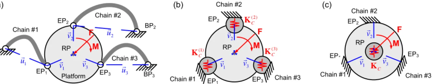
However, for parallel manipulators with passive joints, solutions were obtained for less general cases. They include ―pure‖ parallel architectures where the base and the end platform are connected by strictly serial kinematic chains. Here, the total stiffness matrix can be presented as the sum of partial matrices corresponding to separate chains (computed using the above described technique) 1 1 ( ) θ θ θ q ( ) _C C T q ; T i i i i i i C i i        _ _ ___{ }    _ _



K J K J J K K J 0 (8)

so the passive joints are taken into account easily. Besides, in this case the over-constraining of the mechanism does not create additional difficulties. For instance, for the over-constrained manipulator of Orthoglide family [58], each of the parallel chains yields the stiffness matrix of rank 4 while their aggregation gives the matrix of full rank 6. But if there exists a cross-linking between the parallel chains (like in kinematic parallelograms, for instance), this method can not be applied directly. For this case, some interesting results are presented in [6,41] where the geometrical constraints were treated in a general way but detailed computational techniques were not developed.

VJM modeling of parallel manipulators: problem of internal stresses. In spite of the fact that the VJM technique has

been originally developed for serial manipulators, it can be efficiently applied to parallel robots. The basic idea here is to obtain first the stiffness models of each kinematic chain separately, and after, to integrate them in a united model corresponding to the parallel manipulator. This idea was partially implemented in [3,48], where the manipulator structure was assumed to be strictly parallel (i.e. without internal loops) and the kinematic chains where assembled in the same end-point.

Under such assumptions, the stiffness matrix of the parallel manipulator can be computed via straightforward summation of the chain stiffness matrices

( ) C C 1 n i i 



K K (9)

where the index i defines the kinematic chains and n is the total number of chains. However, in more general (and practically important) cases where the kinematic chains are connected to different points of the end-platform, this formula cannot be applied directly. Besides, for parallel manipulators with parallelogram-based links, some essential modifications are required.

Other limitation of the existing results devoted to the parallel manipulators is related to the assumption that the assembling does not produce any internal stresses. But in practice, numerous errors are accumulated in serial chains [59] and they cause non-negligible internal forces in manipulator joints (even if the external force applied to the end-effector is equal to zero). The internal forces may essentially change the manipulator behavior (modify the stiffness matrix, change the end-effector location, etc.) and should be obviously taken into account in the stiffness model. However, existing works ignore this issue. Another research issue is associated with stiffness modeling of parallel manipulators under loading, which has not received proper attention yet.

(9)

2.3 Stiffness modeling under external and internal loadings

Manipulator stiffness modeling in the loaded mode is a relatively new research area, which is worth to be considered separately. This subsection presents analysis of related works and defines some important research problems that will be in the focus of this work. Some of them are based on the analogy that can be established between robotics and structural mechanics (it concerns buckling phenomena, for instance).

Types of loadings. Manipulator loading may be of different nature. For the stiffness modeling, it is reasonable to distinguish

two main types of loading, external and internal ones. The external loading is caused mainly by an interaction between the robot end-effector and the workpiece, which is processed or transported in the considered technological process [2,26]. Another type of external loading exists due to the gravity influence on the manipulator links, for many heavy manipulators employed in machining the link weight is not negligible [5,7]. Besides, to compensate in a certain degree the gravity influence, some manipulators include special mechanisms generating external forces/torques in the opposite direction. It is worth mentioning that the external loading generated by a technological process is always applied to the manipulator end-effector while others may be applied at intermediate points (at joints, for instance). Besides, the external loadings caused by gravity have obvious distributed nature.

In addition to the above mentioned forces/torques, internal loading in some joints may exists. For instance, to eliminate backlash, the joints may include preloaded springs, which generate the force or torque even in standard "mechanical zero" configuration [9]. Though the internal forces/torques do not influence on the global equilibrium equations, they may change the equilibrium configuration and have influence on the manipulator stiffness properties. For this reason, internal preloading is used sometimes to improve the manipulator stiffness, especially in the neighborhood of kinematic singularities. Another case where the internal loading exists by default, is related to over-constrained manipulators that are subject of the so-called antagonistic actuating [8,60]. Here, redundant actuators generate internal forces and torques that are equilibrated in the frame of close loops. It is obvious that the both external and internal loadings influence on the manipulator equilibrium configuration and, consequently, may modify the stiffness properties. So, they must undoubtedly be taken into account while developing the stiffness model.

Stiffness matrix for the loaded manipulator. At present, in most of related works the stiffness is evaluated in a quasi-static

configuration with no external or internal loading. There is a very limited number of publications that directly address the loaded mode case (or so-called case of ―large deflections‖), where in addition to the conventional ―elastic stiffness‖ in the joints it is

necessary to take into account the ―geometrical stiffness‖ arising due to the change in the manipulator configuration under the

load. Although the existence of this additional stiffness component for elastic structures has been known for a long time [61], the importance of this problem for robotic manipulators has been highlighted rather recently. The most essential results in this area were obtained in [1,2,62] where there are presented both some theoretical issues and several case studies for serial and parallel manipulators. Several authors [8,9,60] addressed the problem of stiffness analysis for the manipulators with internal preloading or antagonistic actuating, but in relevant equations some of the second order kinematic derivates were neglected. Using notation adopted in this work and summarizing existing results [1,2,13], the manipulator stiffness matrix for the loaded can be expressed as follows





-T -1

C  θ θ F θ

K J K K J (10)

where KF is nθnθ stiffness matrix that is induced by external loading and is not presented in previous equation (3). This matrix

depends on both the derivatives of the Jacobian J_θ and the loading vector F. Required details concerning computing of KF are

given in [1].

In the frame of the same concept, the manipulator stiffness model for the loaded mode was proposed in [5,7], where numerous factors were taken into account (conventional external loading, gravity forces, antagonistic redundant actuation, etc.). The final results for the stiffness matrix is presented as

-T 1

C θ u θ





K J K J (11)

where Ku is a solution of a non-linear matrix equation, which includes the joint stiffness and the external/internal loadings as

parameters. However, this approach is rather hard from computational point of view. Besides, in this work the Jacobians and all their derivatives have been computed not in a "true" equilibrium configuration (it was unreasonably replaced by unloaded one). For this reason, since the equilibrium obviously depends on the loading magnitude, some essential issues were omitted. As a result, any nonlinear effects have been detected in the stiffness behavior of the examined manipulators.

Another significant result, which should be mentioned here, is related to the stiffness modeling of the parallel manipulators with the cross-linkage. Firstly this problem was considered in [5,7] where all coordinates where decomposed into two groups (dependent and independent ones). But no clear rule for such coordinate splitting has been proposed, besides the developed

(10)

technique involved very non-trivial computations. Further, the cross-linkage was in the focus of [6,41] where a rather compact expression for the stiffness matrix has been proposed





-T 1 C θ θ F I θ     K J K K K J (12)

which, compared to (10), includes additional matrix KI that is induced by the geometrical constraints (cross-linkage). However,

there are still a number of open questions concerning the coordinate splitting rule (i.e. dividing them into dependent and independent ones) and computing of the equilibrium configuration corresponding to the applied loading.

It should be noted that this problem of (computing the loaded equilibrium) has been omitted in most of the related works. At the same time, it is clear that the changes in the manipulator configuration directly influence the Jacobians (and their derivatives) as well as on the end-effector location. For this reason, computing the Jacobians and Hessians in a traditional way (i.e. for the unloaded configuration) may lead to excessively rough simplification of the stiffness model. In particular, some non-linear phenomena in manipulator stiffness behavior can be hardly detected, while they should obviously exist from the point of view general theory of elastic structures.

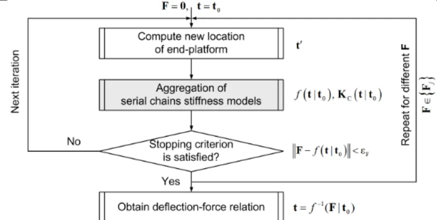
To our knowledge, the most extended results in this area has been presented in [10], where the authors proposed a non-linear stiffness model for parallel manipulators with passive joints which take into account deviations in the manipulator configuration caused by the external loading applied to the manipulator end-effector. In the frame of this conception, an iterative scheme that allows them to compute a static equilibrium configuration has been developed

1 1 q θ q θ 1 q 1 θ θ θ 0 0 0 0 0 0 i i i T i T i                    _{ } _                       F J J t J q J θ q J θ J K K θ (13)

where the vector t defines the end-effector displacement caused by the external loading and θ0 is preloading in virtual springs.

Since, this procedure cannot distinguish a stable equilibrium configuration from an unstable one, there were proposed a matrix criteria that allows user to check stability via analyzing matrix properties

o o o o 0 T F F q F F q q q q                                  V H K H V V H H V (14) where o  V , o q

V are the sub-matrices corresponding to the zero singular values of aggregated Jacobian J, Jq after applying to

it SVD-factorization (see [10] for detail), H_qqF, H_F,H_qF_, H_F_q are the Hessians of scalar function  g q( ,θ)TF with respect to virtual and passive joint coordinates. In accordance with this criteria, the manipulator configuration is stable if (and only if) the matrix (14) is negative-definite. The stiffness matrix for the manipulator with passive joints under the end-point loading can be computed as 1 F T F F C q q T F F T F F F F q q q q q q                            _ _  _ _ _ _ _ _         K J k J J J k H J H k J H H k H (15) where F





1     F

k K H . Among the limitations of the proposed approach it should be mentioned that it is suitable for the manipulators under the loading applied to the end-effector only and with perfect serial chains. These limitations will be overcome in this paper.

Nonlinear-behavior of the manipulator under loading. In mechanics, it has been known since a long time that the elastic

structures may suddenly change their configuration if the loading exceed some critical value. A classical example is the so-called Euler column that retains its straight shape until the loading. This effect (buckling) is well known in structural mechanics, however in robotics this aspect has never been studied before.

Non-linear behavior of force-deflection relation and possible buckling effects have been known since a long time. However in robotics, these questions did not attract much attention, mainly due to high rigidity of commercially available robots. But current trends in mechanical design of manipulators that are targeted at essential reduction of moving masses motivate relaxing this assumption. Hence, non-linear stiffness analysis is also important for the robotic manipulator. As it was mentioned before, existing stiffness analysis techniques for robots are strictly assumed that loading cannot change configurations of an examined manipulator or these changes are negligible. This simplification imposes crucial limitations for the stiffness analysis and, as a result, does not allow us to detect buckling and other non-linear phenomena known from general theory of elastic structures.

(11)

Similar to the classical mechanics three types of buckling can appear in a robotic system: buckling of the link, contact buckling and geometrical buckling. First type of buckling is defined by the mechanical properties of the link and easily can be detected by FEA analysis or critical loading for it can be computed via approximated equations. Normally these loadings are unreachable in robots, while minimization of the link cross-sections can make these limits reachable. Thus it is reasonable to check critical loads for the buckling of elements on the design step. The second type of buckling is caused by the contact of the links with environment. It can be avoided on the machining process designing stage. The nature of the geometrical buckling is closed to the buckling of the elements, while several elements should be analysed together. In this case the critical force is defined by the stiffness of the links and junctions between them. Since stiffness of the junction may be lower than stiffness of links, or even in parallel manipulators can be negligible (for the passive joints), the critical force can be reduced in times comparing with the critical loading of the separate elements. So, nonlinear effects and buckling can appear in robots and they require additional analysis, however these questions have been omitted before.

In practice, it is impossible to detect non-linear effect without finding the loaded equilibrium, while this question was omitted in previous works. Besides, the loading may potentially lead to multiple equilibriums, to bifurcations of the equilibriums and to static instability of the manipulator configurations. These effects are essentialy dangerous for parallel manipulators wich impose numerious passive joints. Some aspects of multiple-equilibrium problem for robotic manipulators have been examined in the works [63,64] who applied the Catastrophe theory for the stability analysis of the planar parallel manipulators with several flexural elements under external loading. However, they did not propose a general approach for stability analysis of the manipulator configurations. Therefore, it will be also in the focus of this research.

3 Stiffness modeling for serial chain with internal and external loadings

Typical examples of the examined kinematic chains can be found in the 3-PUU translational parallel kinematic machine [17], in the Delta parallel robot [65] or in the parallel manipulators of the Orthoglide family [58] and other manipulators [66]. It is worth mentioning that here a specific spatial arrangement of under-constrained chains yields the over-constrained mechanism that posses a high structural rigidity with respect to the external force. In particular, for Orthoglide, each kinematic chain prevents the platform from rotating around two orthogonal axes and any combination of two kinematic chains suppresses all possible rotations of the platform. Hence, the whole set of three kinematic chains produces a non-singular stiffness matrix while for each separate chain the stiffness matrix is singular. This motivated the development of dedicated stiffness analysis techniques that are presented below.

3.1 Problem statement

Let us consider a general serial kinematic chain, which consists of a fixed ―Base‖, a number of flexible actuated joints ―Ac‖,

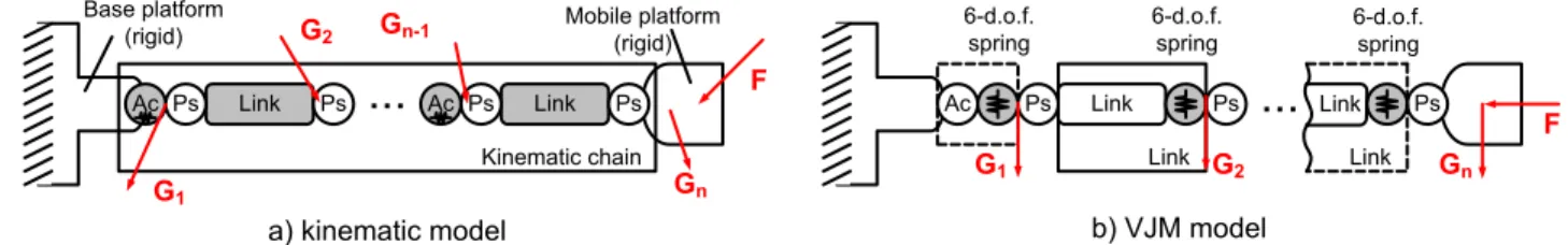
a serial chain of flexible ―Links‖, a number of passive joints ―Ps‖ and a moving ―Platform‖ at the end of the chain (Figure 3). It is

assumed that all links are separated by joints (actuated or passive, rotational or translational) and the joint type order is arbitrary. Besides, it is admitted that some links may be separated by actuated and passive joints simultaneously. Such architecture can be found in most of the parallel manipulators where several similar kinematic chains are connected to the same base and the platform in a different way (with the rotation of 90° or 120°, for instance), in order to eliminate the redundancy caused by the passive joints. It is obvious that such kinematic chains are statically under-constrained and their stiffness analysis cannot be performed by the direct application of the standard methods.

Link

...

Ac Ps Ps Ac Ps Link Ps Kinematic chain Base platform

(rigid) Mobile platform_(rigid)

...

Ps Ps Link Ac Link Link Ps Link 6-d.o.f. spring 6-d.o.f. spring 6-d.o.f. spring

a) kinematic model b) VJM model

G1 G2 F Gn-1 Gn F Gn G2 G1

Figure 3 General structure of kinematic chain with auxiliary loading and its VJM model

In order to evaluate the stiffness of the considered serial chain, let us apply a modification of the virtual joint method (VJM), which is based on the lump modelling approach [39,40]. According to this approach, the original rigid model should be extended by adding virtual joints (localized springs), which describe elastic deformations of the links. Besides, virtual springs are included in the actuating joints, to take into account the stiffness of the control loop. Under such assumptions, the kinematic chain can be described by the following serial structure:

(a) a rigid link between the manipulator base and the first actuating joint described by the constant homogenous transformation matrix TB ase;

(12)

(b) the 6-d.o.f. actuating joints defining three translational and three rotational actuator coordinates, which are described by the homogenous matrix function T_{3 D}(θi_a) where a a a a a a

a ( x , y, z , φx, φy, φz)

i _{   }i i i i _ i _ i



θ are the virtual

spring coordinates;

(c) the 6-d.o.f. passive joints defining three translational and three rotational passive joints coordinates, which are described by the homogenous matrix function T_3D(q_pi) where qi_p (q_xi,qi_y, q_zi,qi_φx,qi_φy,qi_φz) are the passive joint coordinates;

(d) the rigid links, which are described by the constant homogenous transformation matrix _Linki

T ;

(e) a 6-d.o.f. virtual joint defining three translational and three rotational link-springs, which are described by the homogenous matrix function 3 D( L in k)

i

T θ , where θi_Link (   _xi, _yi, _zi, _φxi ,_φyi ,_φzi ), (  _xi, _yi, _zi) and (_φxi ,_φyi ,_φzi )

correspond to the elementary translations and rotations respectively;

(f) a rigid link from the last link to the end-effector, described by the homogenous matrix transformation TT o o l.

In the frame of these notations, the final expression defining the end-effector location subject to variations of all joint coordinates of a single kinematic chain may be written as the product of the following homogenous matrices

 









 



2 1 2



B ase 3 D a 3 D p Lin k 3 D Lin k 3 D p T o o l

i i i i i

i



 



    

T T T θ T q T T θ T q T (16)

where the components B ase, 3D(...), Link, T ool

i

T T T T may be factorized with respect to the terms including the joint variables, in order to simplify computing of the derivatives (Jacobian and Hessian).

This expression includes both traditional geometric variables (passive and active joint coordinates) and stiffness variables (virtual joint coordinates). The explicit position and orientation of the end-effector can by extracted from the matrix T in a standard way [19], so finally the kinematic model can be rewritten as the vector function

( , )



t g q θ (17)

where the vector T ( , )



t p φ includes the position T ( ,x y z, )  p and orientation T x y z (  , , ) 

φ of the end-platform, the vector q(q₁,q₂, ...,q_nq)T contains all passive joint coordinates, the vector T

2 nθ

1

( , , ..., )



θ collects all virtual joint coordinates, nq is the number of the passive joins, nθ is the number of the virtual joints.

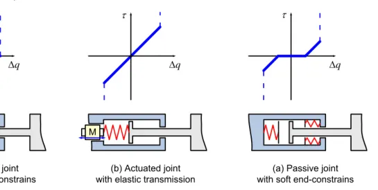
Several examples of prismatic passive and actuated joints are presented in Figure 4a-c , some other types of joints have been illustrated in [67-70]. Such joints include internal springs, as such their statics is described by the following expression





θi Kθi i 0i

     (18)

where _θi is the torque/force caused by the deviation of the joint coordinate i from its unloaded (―zero‖) value 0 i, and

coefficient K_θi defines the spring stiffness. For the purpose of generality, let us introduce similar ―zero‖ values 0 i for the virtual

springs that described flexibility of the links (obviously they are equal to zero for this subset of θ). This allows us to define vector

0

θ of the same size as θ and to present the static equations corresponding to all variables (corresponding to perfect and preloaded passive joints, virtual springs of links and actuators) in general form

θ  θ  ( 0), q  τ K θ θ τ 0 (19)  q   q   q 

(a) Passive joint with hard end-constrains

(b) Actuated joint with elastic transmission

(a) Passive joint with soft end-constrains M

(13)

Here τ_θ,τ_q are the generalized torque/force in joints corresponding to the variables θ and q; the matrix K_θ collects stiffness coefficients of all springs of the kinematic chain. In the frame of this paper it is assumed that the internal loading (which may change the robot stiffness properties) may arise from two reasons: (i) due to additional elastic elements introduced by the designer in order to improve the manipulator properties; (ii) because of internal stresses in links/joints caused by over-constrained architecture of the considered manipulators. It is clear that here the total sum of all internal forces/torques is equal to zero (in contrast to the external loading studied in most of related works); nevertheless the internal loading influence on the manipulator stiffness matrix may be essential.

It is worth mentioning that in the case without internal preloading, the vector θ describes only flexibility of manipulator links/actuators that are presented by virtual springs, while vector q collects entire set of passive joint coordinates. In contrast, here, the passive joint coordinates are divided into two subsets: (i) ―perfect passive joints‖ included in q, and (ii) ―preloaded

passive joints‖ included in θ together with traditional virtual springs. Besides, if a passive joint includes a nonlinear spring (see Figure 4c), the corresponding joint variable may be included either in θ or q, depending on the current configuration of the manipulator. However, for each configuration, this assignment is strictly unique.

It is assumed that the desired stiffness model of serial chain is defined by a non-linear relation

(Δ ) f



F t , (20)

where f(...) is a so-called ―force-deflections‖ function that associates a deflection Δ t with an external force F that causes deformations. It is worth mentioning that the function f(...) can be determined even for the singular configurations (or redundant kinematics) while the inverse statement is not generally true. Hence, enhanced stiffness analysis must include the computation of this function and the detailed analysis of its singularities that may provoke various nonlinear phenomena (such as buckling). In the unloaded case, this function is usually defined through the ―stiffness matrix‖ K , which describes the linear relation

0 0 ( , ) Δ

 

F K q θ t between small six-dimensional translational/rotational displacements Δ t, and the external forces/torques F

causing this transition. Here, it is assumed that Δ t includes three positional components (  x, y, z) describing the displacement in Cartesian space and three angular components (Δx, Δy, Δz) that describe the end-platform rotation around

the Cartesian axes, while the vectors q0,θ0 correspond to the manipulator equilibrium configuration for which the loadings (both

internal and external) are equal to zero. However, for the loaded mode, similar linear relation is defined in the neighborhood of another static equilibrium, which corresponds to a different manipulator configuration ( , )q θ , that is modified by external forces/torques F . Respectively, in this case, the stiffness model describes the relation between the increments of the force Fand the position t

( , )

F

 

F K q θ t (21)

where qq0Δq and θθ0Δθ denote the new configuration of the manipulator, and Δq, Δ θ are the deviations in the

coordinates q,θ respectively.

For stiffness modeling of serial kinematic chain with auxiliary loading let us assume that the serial chain has the additional external loadings applied to the internal node points (Figure 3). These loadings can be caused by gravity forces (generally they are distributed, but in practice they can be approximated by localized ones) and/or gravity compensators. These forces will be denoted as G_j, where j1, ...,n is the node number in the serial chain starting from the fix base (here, jn corresponds to the end-point). It should be noted that for computational convenience, it is assumed that the end point loading consists of two components Gn and F of different nature.

It is evident that in general the auxiliary forces Gi depend on the manipulator configuration. So, let us assume that they are

described by the functions

( , )

j  j

G G q θ , (22)

In contrast, for the external force F, it is assumed that there is no direct relation with the manipulator configuration.

For the serial chains with the auxiliary loadings it is also required to extend the geometrical model. In particular, in addition to the equation (17) defining the end-point location, it is necessary to introduce the additional functions

( , ), 1, ...,

j  j j n

t g q θ (23)

defining locations of the nodes. It is worth mentioning that for the serial chain, the position tj depends on a sub-set of the joint

coordinates (corresponding to the passive and virtual joints located between the base and the j-th node), but for the purpose of analytical simplicity let us use the whole set of the joint coordinates ( ,q θ) as the arguments of the functions gi(...).

Using these assumptions, the problem of stiffness modeling of serial chains with auxiliary loadings can be split in the following sub-problems: (a) deriving the static equilibrium equations for the chain with auxiliary loadings; (b) computing

(14)

full-scale “force-deflections relation‖ for the end-point and intermediate nodes; (c) linearization of the relevant force-deflection relations in the neighborhood of the equilibrium and computing corresponding stiffness matrix. Let us focus on these sub-problems.

3.2 Static equilibrium equations for serial chain with auxiliary loadings

To obtain a desired stiffness model, let us derive first the static equilibrium equations. In the frame of this work, the notion of static equilibrium of serial chain is referred to the configuration (defined by a set of the actuated, virtual and passive joint coordinates) that depends on external/auxiliary loadings, which ensure zero sums of forces/torques for each link separately. Let us apply the principle of the virtual work and assume that the kinematic chain under external loadings F and G 



G₁...G_n



has the configuration



q,θ



and the locations of the end-point and the nodes are tg q( , )θ and t_j g_j( , ),q θ j1,n respectively. According to the principle of virtual work, the work of external forces G F, is equal to the work of internal forces τ_ caused by displacement of the virtual springs θ



T



T T θ 1 n j j j     



G t F t τ θ (24)

where the virtual displacements tj can be computed from the linearized geometrical model derived from (23)

( ) ( )

θ q , 1..

j j

j     j n

t J θ J q , (25)

which includes the Jacobian matrices









( ) ( ) θ , ; q , j j j j       J g q θ J g q θ θ q (26)

with respect to the virtual and passive joint coordinates respectively. Substituting (25) to (24) we can obtain the equation



T ( ) T ( )

 

T ( ) T ( )



T θ q θ q θ 1 n j j n n j j j             



G J θ G J q F J θ F J q τ θ (27)

which has to be satisfied for any variation of θ, q. It means that the terms regrouping the variables θ, q have the coefficients equal to zero, hence the force-balance equations can be written as

( ) T ( ) T ( ) T ( ) T θ θ θ q q 1 1 ; n n j n j n j j j j 



   



   τ J G J F 0 J G J F. (28)

Also, these equations can be re-written in block-matrix form as

(G ) T (F) T (G ) T (F) T θ  θ   θ  ;  q   q  τ J G J F 0 J G J F (29) where (F) ( ) ( ) ( ) (G ) (1)T ( ) T (G) (1) ( ) T T θ θ q q θ θ θ q q q 1 T T T T T ; ; ... ; ... ; ... n F n n n n          _ _ _ _ _ _ J J J J J J J J J J G G G (30)

Finally, taking into account the virtual spring reaction



0



θ  θ 

τ K θ θ , where





1 n

θ diag θ, ..., θ

K K K , the desired static equilibrium equations can be presented as





(G ) T (F ) T 0 θ θ θ (G ) T (F ) T q q           J G J F K θ θ J G J F 0 (31)

It should be noted that compared to the case of end-effector loading only [10], here there are two additional terms (G ) T

θ

J G and

(G ) T q

J G that take into account the influence of the auxiliary loading G . Further, these equations will be used for computing the static equilibrium configuration and corresponding Cartesian stiffness matrix.