A Comparison of Imputation Strategies in Cluster Randomized Trials with Missing Binary Outcomes

(1)

HAL Id: hal-03157717

https://hal.archives-ouvertes.fr/hal-03157717

Submitted on 31 Mar 2021

HAL is a multi-disciplinary open access archive for the deposit and dissemination of sci-entific research documents, whether they are pub-lished or not. The documents may come from

L’archive ouverte pluridisciplinaire HAL, est destinée au dépôt et à la diffusion de documents scientifiques de niveau recherche, publiés ou non, émanant des établissements d’enseignement et de

A Comparison of Imputation Strategies in Cluster

Randomized Trials with Missing Binary Outcomes

Agnès Caille, Clémence Leyrat, Bruno Giraudeau

To cite this version:

Agnès Caille, Clémence Leyrat, Bruno Giraudeau. A Comparison of Imputation Strategies in Cluster Randomized Trials with Missing Binary Outcomes. Statistical Methods in Medical Research, SAGE Publications, 2016, 25 (6), pp.2650–2669. �10.1177/0962280214530030�. �hal-03157717�

(2)

A comparison of imputation strategies in cluster randomized trials with missing binary outcomes

Agnès Caille, 1,2,3,4 Clémence Leyrat, 1,2,3 and Bruno Giraudeau1,2,3,4

1. INSERM, UMR-S 738, Paris, France 2. INSERM, CIC 202, Tours, France 3. CHRU de Tours, Tours, France

4. Université François-Rabelais de Tours, PRES Centre-Val de Loire Université, Tours, France

Address for correspondence:

Agnès Caille INSERM CIC 202 2 Bd Tonnellé 37044 Tours cedex 9 France Tel: 33 (0)2 34 37 96 54 Fax: 33 (0)2 47 47 46 62 agnes.caille@med.univ-tours.fr

(3)

Abstract

In cluster randomized trials, clusters of subjects are randomized rather than subjects themselves, and missing outcomes are a concern as in individual randomized trials. We assessed strategies for handling missing data when analysing cluster randomized trials with a binary outcome; strategies included complete-case, adjusted complete-case, and simple and multiple imputation approaches. We performed a simulation study to assess bias and coverage rate of the population-averaged intervention effect estimate. Both multiple imputation with a random-effects logistic regression model or classical logistic regression provided unbiased estimates of the intervention effect. Both strategies also showed good coverage properties, even slightly better for multiple imputation with a random-effects logistic regression approach. Finally, this latter approach led to a slightly negatively biased intracluster correlation coefficient estimate but less than that with a classical logistic regression model strategy. We applied these strategies to a real trial randomizing households and comparing ivermectin and malathion to treat head lice.

Keywords

(4)

1. Introduction

Cluster randomized trials (CRTs), in which clusters of subjects are randomized rather than subjects themselves, are being increasingly used to assess health promotion or health services organization interventions.1 The cluster design may be motivated by different reasons. Some interventions apply to the cluster level, such as the implementation of guidelines, which prevents randomizing individuals. Cluster randomization is also adopted to avoid bias due to contamination between groups, which can be due to a "herd effect" because of interactions between members of clusters, or because the study deals with an infectious disease such as influenza, lice or scabies.2–4 One feature of CRTs is the presence of correlation among outcomes of subjects within each cluster, which is usually quantified by the intracluster correlation coefficient (ICC). Such a correlation must be taken into account in CRTs, both when planning, to have nominal power, and during the statistical analysis, to prevent type I error inflation.5

Otherwise, CRTs, as do any randomized clinical trial, incur missing outcomes,6 with sometimes outcomes missing for entire clusters.7 Complete-case (CC) analysis, in which subjects with a missing outcome are excluded, is often performed. However, such an analysis strategy has several pitfalls: it leads to loss of power8 and usually provides biased estimates of the intervention effect.6,9 In the end, excluding subjects with a missing outcome does not respect the intention-to-treat principle, which requires each randomized subject (and cluster) to be taken into account in the statistical analysis, including subjects for whom the outcome is missing.10–12 To respect this methodological cornerstone of the analysis of randomized trials, the imputation of missing outcomes is required.13

We investigated different methods for handling missing binary outcomes in CRTs and assessed their impact on both the intervention effect and ICC estimates. Section 2.1 presents the real CRT that motivated our research and section 2.2 provides the statistical analysis method for the outcome in the absence of missing data. Section 3 defines the different strategies evaluated for handling missing outcomes. Section 4 describes a simulation study and presents the results with use of the different strategies. In section 5, these strategies are applied to our real CRT example, as a sensitivity analysis. Finally, section 6 discusses our results.

(5)

2. Motivating example: the ivermectin trial and analysis method 2.1 Trial design

A recent CRT motivated our research.14 This multicenter double-blind double-dummy study enrolled 812 subjects in 376 households with difficult-to-treat head-lice infestation. Each household was randomly assigned such that any infested subject within the household received oral ivermectin or malathion lotion. The primary outcome was the absence of head-lice on day 15. In this trial, a cluster design was used to prevent contamination between the two groups within the household, head-lice infestation being readily transmissible. A more detailed description of this trial can be found in Chosidow et al.14 In all, 398 subjects in 185 households were randomly assigned to receive ivermectin, and 414 subjects in 191 households were randomly assigned to receive malathion. In the ivermectin group, one subject (the only individual in that household) who did not receive any treatment and was not seen on day 15, was excluded from the analysis. Such an exclusion did not compromise the internal validity of the trial because of blindness (i.e., the reason for not being treated is independent from the allocation group).15 On day 15, 42 (10.6%) primary outcomes were missing for patients in the ivermectin group and 46 (11.1%) in the malathion group. In the complete-case population, the success rate was estimated at 90.0% for the malathion group and 97.2% for the ivermectin group. Considering Y , the outcome from subject l _ijl (l = 1,…, mij) in cluster j (j = 1,…, k) randomized in group i (i = 0 in the control [malathion]

group and i = 1 in the intervention [ivermectin] group), we defined R , the missing data ijl indicator for the binary outcome Y , as _ijl R_ijl =1 if the primary binary outcome Y is observed _ijl and Rijl =0 if Y is missing. We estimated τ, the ICC for the missing data indicator ijl R .ijl

16 τ was estimated at 0.85 (95% confidence interval [95% CI] [0.72-0.92]), which is consistent with the fact that the outcome was missing for the entire cluster in 34 clusters of the 43 clusters with at least one missing outcome (79.1%). We assessed which individual baseline covariates were associated with the outcome and/or with the missing data indicator. We found that age, hair length, severity of infestation and hair density were predictors of success (among subjects with observed outcome). Age and severity of infestation were predictors of missingness. Body mass index (BMI) and sex were predictors of neither success nor missingness.

(6)

2.2 Statistical analysis of binary outcome in the absence of missing data A generalized estimating equation (GEE) approach can be used to estimate the population-average (PA) (also called marginal) intervention effect.17,18 The logistic model is as follows:

i PA PA ijl ijl G P P ₍ ₎ ₍ ₎ ) 0 ( 1 log _=β +β       − (1)

where Pijl =E(Yijl) is the marginal probability of success for subject l in cluster j of group i;

ijl

Y , the binary outcome of interest (equals to 1 with absence of head lice at day 15 and 0 otherwise); G , the group dummy variable (0 for subjects in the control group and 1 for _i subjects in the intervention group); ( )

) 0 (

PA

β , the marginal log odds of the probability of success in the control group (with the PA exponent referring to "population-average"); and

β

( PA), the marginal log-odds ratio of success between the intervention and control groups. To account for clustering, we used the robust variance estimator for standard error and specified an exchangeable correlation structure.

The ICC must be estimated as recommended in the CONSORT Statement extension for CRTs.19 The Fleiss and Cuzick estimator20 for binary outcomes can be used.

3. Missing Data Management Strategies

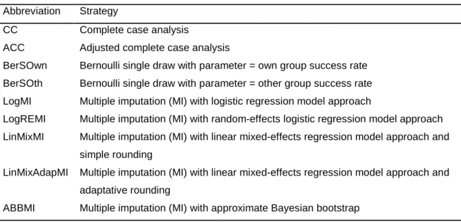
In this paper, we considered nine strategies to manage missing outcomes. The abbreviations used for the missing data strategies are in Table 1. These strategies can be separated as CC analysis, single imputation (SI) and multiple imputation (MI) strategies. Accuracy of these strategies to handle missing data is closely related to the missingness mechanism. Three categories of missing data mechanism were introduced by Little and Rubin.21 Data are said to be missing completely at random (MCAR) if missingness is independent of both unobserved and observed data, which is rare in practice,22 and missing at random (MAR) if, given the observed data, missingness is independent of the unobserved data. Finally, data are said to be missing not at random (MNAR) if they are neither MCAR nor MAR. In the case of partially observed outcome but fully observed covariates, a CC analysis, in addition to its association with loss of power, leads to a biased intervention-effect estimate unless (i) the outcome is MCAR or (ii) the outcome is MAR given some covariates that are included (adjusted for) in the analysis model (adjusted CC) or (iii) the outcome is MNAR dependent only on outcome and a crude odds ratio is estimated. The latter case is explained by the symmetry property of the odds ratio.23 MI strategies rely on the assumption that data are MAR.6 Moreover, to be

(7)

congenial with the analysis, as defined by Meng,24 the MI model for CRTs needs to reflect the multilevel structure of the data (i.e., to account for intracluster correlation).25

3.1 Complete Case Analysis

In CC strategies, no imputation is performed, and only data from subjects with an observed outcome are considered for the statistical analysis.

3.1.1 Complete case analysis (CC)

CC analysis is the simplest and widely used approach: data from any subject with a missing outcome are discarded before fitting the model.

3.1.2 Adjusted complete case analysis (ACC)

When outcomes are missing at random (MAR), a CC analysis with an adjustment for covariates provides an unbiased estimate of the intervention effect.22 For the ACC strategy, the following model is fitted to the subjects with observed outcomes:

ijl n PA n ijl PA i PA PA ijl ijl X X G P P ) ( ) ( ) ( ) 1 ( ) ( ) 1 ( ) ( ) ( ) 0 ( ... 1 log _=β +β +β + +β       − (2)

where (X₍₁₎,...,X₍_n₎) are n individual covariates predictive of missingness and

(

_{( )} ( )

)

) ( ) ( 1 ,... PA n PA β β

are associated parameters.

3.2 Single imputation strategies

In SI strategies, each missing outcome is replaced only once.

3.2.1 Bernoulli single-draw-based strategy with own group success rate as parameter (BerSOwn)

In this strategy, we use an informal imputation method, with the same approach as proposed by Wittes.26 For each missing outcome, a value is imputed with a Bernoulli draw. The parameter of the probability distribution is specific to each group. For the control group, the parameter equals the observed success rate over complete cases from the control group, and the same approach is used for the intervention group.

3.2.2 Bernoulli single-draw-based strategy with other group success rate as parameter (BerSOth)

This strategy is the same as previously described except for the parameter of the Bernoulli distribution. For patients in the control group, the parameter used is the observed success rate over complete cases from the intervention group, and vice versa. Thus, one can expect this

(8)

3.3 Multiple imputation strategies

SI strategies prevent loss of power but are known to lead to undercoverage, as they cannot reflect missing outcome uncertainty and thus underestimate the variance of intervention-effect estimates.8 In MI strategies, each missing outcome is replaced D > 1 times, which accounts for the uncertainty of imputed values by incorporating the between-imputation variance to standard variance estimation.27 Therefore, D completed datasets are generated, and each one is analysed, thus producing D intervention-effect estimates and their standard errors. For all MI strategies used in our work, each of the D completed datasets is analyzed with the model (1). These D estimates are then combined according to Rubin's rules to obtain one intervention effect estimate.27

3.3.1 MI with random-effects logistic regression model (LogREMI)

In this strategy, we consider the following random-effects logistic regression model, also called cluster-specific (CS) model,28 to generate multiple imputations:

ij ijl n CS n ijl CS i CS CS ijl ijl c X X G P P + + + + + =         − ( ) ) ( ) ( ) 1 ( ) ( ) 1 ( ) ( ) ( ) 0 ( ... 1 log β β β β , (3)

where

β

(CS) is the CS log-odds ratio of success between the intervention and control groups, (X₍₁₎,...,X₍_n₎) are the n individual covariates previously defined,

(

_{( )} ( )

)

) ( ) ( 1 ,... CS n CS β β are the

associated parameters and c is the random cluster effect associated with cluster j within _ij group i, and distributed as N(0,σ_c2).

Imputed values are generated by adapting, to the specific context of a CRT, a method proposed by Carpenter and Kenward29 in the context of a longitudinal study with missing binary outcomes.

The following steps are performed:

(1) Model (3) is fitted using SAS NLMIXED to the observed data to obtain estimates of Β(CS)

where Β(CS) refers to the (n+2)-vector ( (() ) ) ( ) ( ) 0 ( , ,..., CS n CS CS

β

) of fixed parameters and their

covariance matrix Σ_β( CS) .

) (CS

Β starting values are obtained from the ACC strategy model (2) and a grid search is used for the starting value of 2

c

σ . The "predict" option is used to obtain the cluster-specific random effects cˆ and associated variance estimate _ij ˆ2

ij c

σ

, regardless of whether the cluster has subjects with missing outcomes or not.

(9)

(2) Then, the next steps are repeated D times: a. Draw (CS)*

Β from a multivariate normal distribution (ˆ ,ˆ ( ))

) (

CS CS

N Β Σ_β and, for each cluster j with at least one subject with a missing outcome, draw c*_ij from

) ˆ , ˆ ( ij c ij c N σ .

b. For each subject l with a missing outcome (i.e., Rijl =0), calculate the individual predicted probability of a success as follows:

*

ijl

p = expit(

β

₍(₀CS₎ )* +

β

(CS)*g_i +

β

₍(₁CS₎ )*x₍₁₎_ijl +...+

β

₍(_nCS₎)*x₍_n₎_ijl +c_ij*), with expit(x = ) ) 1 ( 1 ) ( x e− + .

Finally, draw the imputed oucome for subject l from a Bernoulli with parameter p_ijl* .

c. The (2) b step is repeated for each subject with a missing outcome to obtain the Dth completed data set.

As denoted by Carpenter and Kenward,29 such an approach is only an approximate proper imputation procedure because to obtain the Dth completed data set, cˆ and _ij ˆ2

ij c

σ

are not re-estimated after

β

(CS)* has been drawn. A SAS macro to implement this strategy is available upon request from the first author.

3.3.2 MI with logistic regression model (LogMI)

In this strategy, imputed values are generated with the following standard logistic regression model, which does not account for the intracluster correlation:

ijl n n ijl i ijl ijl X X G P P ) ( ) ( ) 1 ( ) 1 ( ) 0 ( ... 1 log _=β +β +β + +β       − . (4)

The following steps are performed:

(1)Model (4) is fitted to the observed data to obtain estimates of Β the (n+2)-vector (

β

₍₀₎,

β

,...,

β

₍_n₎) of fixed parameters and their covariance matrix _{Σ .}_β

(2)Then, to generate imputed binary outcomes, the next steps are repeated D times: a. Draw Β from the posterior distribution of Β approximated by a multivariate *

(10)

b. For each subject l with a missing outcome (i.e. Rijl =0), calculate the individual predicted probability of a success as follows:

*

ijl

p = expit(

β

₍*₀₎ +

β

*g_i +

β

₍*₁₎x₍₁₎_ijl +...+

β

₍*_n₎x₍_n₎_ijl) Finally, draw the imputed oucome for subject l y_ijl* as

     _< = otherwise, 0 , if 1 * * ijl ijl ijl p u y

where u_ijl is a draw from a uniform distribution between 0 and 1.

c. The (2) b step is repeated for each subject with a missing outcome to obtain the Dth completed data set.

This strategy, although uncongenial with the substantive model can be implemented with SAS PROC MI.

3.3.3 MI with linear mixed-effects regression model and simple rounding (LinMixMI)

A normal distribution may be accurate to impute binary variables.30,31 In this strategy, the following linear mixed-effects regression imputation model is considered:

ijl ij ijl n n ijl i ijl G X X U e Y =α(0) +α +α(1) (1) +...+α( ) ( ) + + , (5)

where

α

is the intervention effect, (X₍₁₎,...,X₍n₎) are the n individual covariates previously defined,

(

α₍₁₎,...α₍_n₎

)

are the associated parameters, U is the random cluster effect associated _ij with cluster j within group i, and distributed as N(0,σb2) and e is the residual error related ijl to subject l in cluster j within group i, and distributed as N(0,σw2).

We use the Markov chain Monte Carlo (MCMC) algorithm developed and implemented by Schafer31 in the R package "pan". The procedure is more complex than in Section 3.3.1 because it can provide multiple imputations of missing values on multiple variables (not only the outcome) with non-monotone patterns. In our univariate case, given the observed outcomes Yobs, current versions of the parametersΑ,σb2,σw2 [where Α refers to the (n+2)-vector (

α

(0),

α

,...,

α

(n)) of fixed parameters], the random effects U , and the missing ij outcomes Ymiss are updated in three steps:

(1) U are drawn given plausible assumed values for the missing outcomes _ij Y_miss and the parameters Α,σ_b2,σ_w2; then,

(11)

(2)New random values are drawn for the parameters Α,σ_b2,σ_w2 given assumed values for the missing outcomes Y_missand the random effects U achieved in (1); and finally, _ij (3)New random values are drawn for the missing outcomes Y_miss given the random effects

ij

U achieved in step (1) and the parameters Α,σb2,σw2 achieved in step (2).

These three steps, corresponding to a Gibbs sampler cycle, are repeated with large number of iterations for the simulated parameter values to finally converge in distribution to their correct posterior distributions.

This strategy takes the intracluster correlation into account but, as it considers that Y is _ijl normally distributed, it imputes a continuous value for each missing outcome, which is then rounded off to 0 or 1. Here, a simple rounding, with imputed values rounded to 1 if ≥ 0.5 and to 0 otherwise, is used.

3.3.4 MI with linear mixed-effects regression model and adaptative rounding (LinMixAdapMI)

In this strategy, imputed values for the missing outcomes Ymiss are the same as in Section 3.3.3. The difference with the previous strategy relies on the rounding method: here, the adaptative rounding method proposed by Bernaards30 is used in which the dichotomization threshold relies on marginal prevalence of success observed on the completed binary outcome dataset. The adaptative-rounding dichotomization threshold is obtained as follows:

(1)Calculate ω, the mean value of Y (on observed binary outcomes and imputed _ijl values) then,

(2)Calculate t, the adaptative rounding threshold, based on a normal approximation to the binomial distribution, as t=

ϖ

−Φ−1(

ϖ

)

ϖ

(1−

ϖ

), where Φ−1 is the quantile function of the normal distribution and finally,

(3)Round imputed outcome to 1 if imputed value is ≥ t and round imputed outcome to 0 if imputed value is < t.

For a binary outcome with extreme prevalence (rare or frequent), this method is assumed to perform better.

3.3.5 Approximate Bayesian bootstrap MI (ABBMI)

This strategy is a non-parametric MI approach.32,33 The following steps are performed to impute the missing outcomes:

(12)

(1)First, a propensity score is generated to estimate the probability of missingness for an outcome given the observed n individual covariates by fitting the following logistic regression model: ijl n n ijl i ijl ijl X X G R P R P ) ( ) ( ) 1 ( ) 1 ( ) 0 ( ... ) 0 ( 1 ) 0 ( log _=θ +θ +θ + +θ       = − = .

(2)Then, five strata are defined using the quintiles of the propensity score obtained in step (1).

(3)Finally, in each stratum, an approximate Bayesian bootstrap is performed. First, Yobs

draws with replacement are made on the Yobs observed outcomes to obtain a pool of

plausible values. Then, the values for the Ymis missing outcomes are sampled with

replacement in the pool of Yobs values previously obtained to provide a completed

dataset. These two sampling procedures are repeated D times to obtain D completed datasets.

This strategy can be implemented with SAS PROC MI. 4. Simulation study

4.1 Simulation design

We simulated complete CRTs with two parallel groups of 500 subjects per group and varying cluster sizes. We first generated CRTs with a continuous outcome, which we further dichotomized to obtain a binary outcome with pre-specified success rates. Once the complete CRTs were obtained, we generated an individual missing data indicator to obtain a follow-up rate π = 0.8 (i.e., 20% of missing binary outcomes) with an MAR mechanism.

4.1.1 Complete dataset generation

Our simulation plan was adapted from Leyrat et al.34 The following simulation steps were used:

(1)Each cluster size, mij, was first randomly generated from a Poisson distribution of

parameter m (i.e., the mean cluster size) as was previously proposed to yield varying cluster sizes.18

(2)Individual continuous outcomes were simulated according to the following model: ijl ij i c ijl G U e Y =

α

₍₀₎ +

α

+ + ,

where

α

is the intervention effect for the continuous outcome Y_ijlc (with the c exponent referring to continuous). For convenience and without loss of generalizability, we set

0

0 =

(13)

) ( ) ( ₁ 1 ₀ 1 P P − − ₋_Φ Φ =

α to obtain success rates equal to pre-specified values of P and 0 P1

in the control and intervention groups, respectively.

(3)Individual covariates mimicking BMI, age, hair length, sex, severity of infestation and hair density were generated as follows:

a. First, six standard normally distributed covariates X₍_p₎

(

p=1,L,6

)

were generated with Pearson's correlation r_{( p}₎ between the covariate and the continuous outcome of r = 0 for BMI, ₍₁₎ r(2) = 0.4 for age, r(3) = −0.4 for hair

length, r(4) = 0 for sex, r(5) = −0.4for severity and r(6) = 0.4 for hair density.

b. The last three covariates were further dichotomized with adequate threshold values to obtain the same prevalence as in our motivating trial, for sex (87% of girls), severity (38% of severe infestation) and hair density (47% of thick hair), respectively.

(4)The individual continuous outcome Y_ijlc was finally dichotomized to obtain a binary outcome Y with success rates equal to pre-specified values of ijl P and 0 P1.

4.1.2 Missing data introduction

Once the complete datasets were simulated, we introduced missing outcomes by generating the individual missing data indicator R as follows: _ijl

(1)Let η_ij be the rate of observed outcomes for cluster j in group i being distributed as a Beta distribution with parameter a and b defined as:

τ τ π(1− ) = a , and τ τ π)(1 ) 1 ( − − = b ,

where π is the rate of observed data (π=0.8) and τ is the ICC for the missing data indicator. (2)Let define Z as: _ijl

ijl

Z = logit

{

P

(

R_ijl =1

)

}

=

γ

₍_age₎_iAge_ijl +

γ

₍_sev₎_iSeverity_ijl +

λ

_ij

where _       − = ij ij ij η η λ 1

log is a random cluster effect.

(3)Finally, for each subject l, we draw r as Bernoulli with parameter (expit(_ijl z )). If ijl

ijl

r =0 the outcome for subject l was missing and if r =1 the outcome for subject l was ijl observed.

(14)

Our missing data introduction procedure implies that the missing data mechanism is MAR depending on two covariates, age and severity of infestation, as in our motivating trial, and that it takes into account the ICC for the missing data indicator.

4.1.3 Simulation parameters

The ivermectin trial estimates were used to calibrate the simulation plan. Thus, we first considered a CRT with k = 200 clusters per group; success rates (P , ₀ P₁) = (0.90, 0.97) in the control and intervention groups, respectively; an ICC for the binary outcome in the control group ρ = 0.40; and an ICC for the missing data indicator τ = 0.85. We fixed parameters for age at γ_(age₎₀ = log(2), γ_(age₎₁ = 0 and for severity at γ_{( sev}₎₀ = 0 and γ_(sev₎₁ = log(5). This corresponds to an odds ratio relating missingness and age of 1/2 = 0.5 in the control group and 1 in the intervention group. For severity, these parameters correspond to odds ratios of 1 in the control group and 1/5 = 0.2 in the intervention group. We also explored other realistic scenarios that differed from our example, especially smaller values for the binary outcome ICC, which are more plausibly observed.35

Simulation parameters were then specified as follows:

• Number of clusters per group (k), mean number of subjects per cluster (m): (k,m) = (200,2.5) and (40,12.5).

• Success rates in the control and intervention groups: (P , ₀ P₁) = (0.50, 0.57) and (0.90, 0.97), which correspond to the expected regression coefficients

β

( PA) of 1.279 and 0.282, respectively (and values of 3.59 and 1.33 in terms of odds ratios).

• ICC for the binary outcome in the control group: ρ = (0.05, 0.01). For a binary outcome, ρ depends on the success rate, so it is expected to be different in the intervention and control groups.36 We controlled and explored only the value of ρ in the control group. Because we first generated a continuous individual outcome, we specified the ICC value for the continuous outcome so that it allows for recovering the pre-specified ICC value for the binary outcome.37 For this, we used the attenuation formula proposed by Kraemer,38 shown to be accurate for CRTs with variable cluster size.39

• ICC for the missing data indicator: τ = (0, 0.1, 0.3, 0.8).

The combination (k,m) = (200,2.5) and ρ = (0.01) was not simulated because as the ICC value depends in part on cluster size, this small value seemed unrealistic.35 For each combination of simulation parameters, 1 000 datasets were simulated by using SAS.

(15)

4.1.4 Implementation

Each of the nine missing data strategies was then applied to the simulated incomplete datasets. We used the SAS PROC GENMOD with REPEATED statement to fit models (1) and (2). For MI strategies, we generated D = 20 imputed datasets for each simulated dataset. Missing data were imputed in R for the LinMixMI and LinMixAdapMI strategies using the package "pan". The first 1 000 iterations were considered burn-in, 100 updates then separated each saved draw from the posterior distribution, and prior "guesstimates" for variance parameters were obtained from expectation-maximization algorithms also implemented in the package "pan". The imputed values were then imported in SAS to be rounded, analysed and results combined. All other missing data strategies were performed entirely with SAS.

4.1.5 Performance criteria

The nine missing data handling strategies were evaluated based on:

• Relative bias defined as:

) ( ) ( ) ( ˆ 100 _PA PA PA β β β − × where β_ˆ(PA)

is the average of the estimated intervention effect over the 1 000 simulations. A positive relative bias means an overestimation of the intervention effect and vice versa.

• Average estimated standard error of the intervention effect estimate defined as:

∑

= 1000 1 ) ( ) ˆ ( 1000 1 i PA i SE β .

• Coverage rate of the regression coefficient defined as the proportion of 95% CIs containing the true regression coefficient value. The margin of error with 1 000 simulation replicates is 1.96 0.05×0.951000=0.014 for the coverage of nominal 95% CIs. Thus, we considered a coverage rate smaller than 93.6% as undercoverage and greater than 96.4% as overcoverage.

• Estimated ICC for the binary outcome defined as ρˆ , the average of the estimated ICC over the 1 000 simulations. The MI estimator for the binary outcome ICC was simply the average of the D estimates.

• For MI strategies, we also estimated the fraction of missing information (FMI), which relies on the ratio of the between-imputation variance to the within-imputation variance and reflects how missing information contributes to inferential uncertainty

(16)

imputations, as compared to an infinite number of imputations, is approximately

(

)

1

1+FMI D − .40

4.2 Simulation results

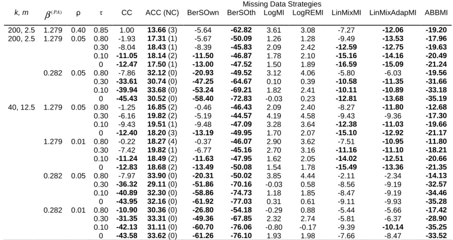
4.2.1 Relative bias of intervention effect

Table 2 displays the relative bias of averaged intervention effects. When (P , 0 P1) = (0.90, 0.97), we sometimes encountered convergence problems (although rarely)

for the ACC strategy (and therefore for the LogREMI strategy) because of the limited number of pejorative outcomes. For the CC strategy, whatever the value of k, m,

β

( PA) and ρ, relative bias decreased with increasing τ, the ICC for missing data indicator. Indeed, with increasing τ, outcomes within a cluster tend to be fully observed or fully missing, so individual covariates have lower influence on the missingness process.

Regarding the ACC strategy, for a given

β

( PA), relative bias was not influenced by parameters k, m, ρ and τ. Otherwise, this strategy was associated with a mean intervention-effect estimate systematically higher than that associated with the CC strategy. Indeed, because of the noncollapsibility of the odds ratio, the

β

( PA) estimate associated with the ACC strategy was expected to be farther from the null than the

β

( PA) estimate associated with the CC strategy.22 LogMI and LogREMI were the least biased strategies: relative bias was lower than 5% in any situation. In contrast, BerSOth and ABBMI were highly biased strategies, whatever the simulation scenario, and BerSOwn, LinMixMI and LinMixAdapMI provided acceptable bias in few situations.

4.2.2 Average standard error and coverage rate of 95% CIs

Tables 3 and 4 display the average estimated standard errors of intervention-effect estimates and coverage rates of 95% CIs. Average standard errors were slightly larger for LogREMI, which accounts for intracluster correlation than for LogMI. For a given

β

( PA), the relative difference in average standard errors between LogMI and LogREMI increased with ρ. Nevertheless, these two strategies produced CIs with good coverage properties and as expected, even better for LogREMI than for LogMI. LinMixMI and LinMixAdapMI showed reasonable coverage properties in most scenarios. All other strategies resulted in poor coverage properties. ACC, which adjusts on covariates that are associated with the outcome, resulted in greater average standard errors than the unadjusted CC. Single imputation

(17)

strategies, BerSOwn and BerSOth, led to low coverage rates because of a bias in the estimated intervention effects and an underestimation of the standard errors.

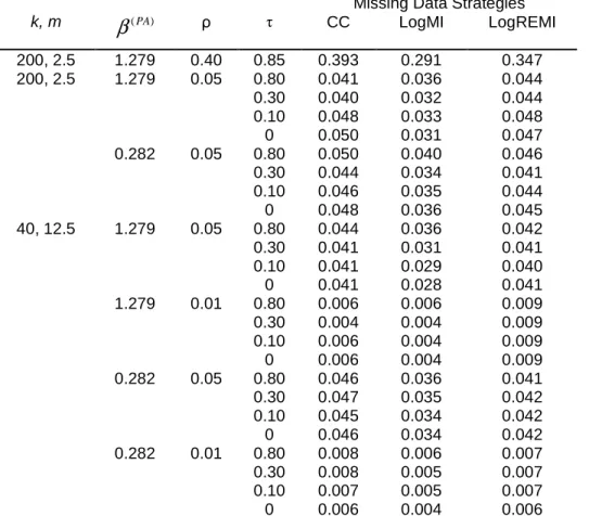
4.2.3 ICC for the binary outcome

Table 5 displays the estimated ICC in the control group averaged over the 1 000 simulations. We report only the results obtained for the strategies with the best results regarding correction of bias and coverage rate, namely LogMI and LogREMI, which we compared with the CC strategy. As expected, estimates for the LogMI strategy, which does not account for the ICC were attenuated as compared with the LogREMI strategy, and this attenuation increased at larger ρ value. For the values considered in our study, the CC strategy also provided consistent estimates for ρ.

4.2.4 Fraction of missing information

Over all scenarios, the fraction of missing information was mainly less than 0.15 (Table S1 in the online supplementary material) with maximal value 0.22. Therefore, estimates based on 20 imputations had a relative efficiency of 99% in unit variance and thus a standard deviation that is, at most, 0.5% higher than those based on an infinite number of imputations.

5. Application of the missing data handling strategies to the Ivermectin trial data

The nine missing data handling strategies were applied to the data from the trial described in Section 2. The intervention group and six baseline covariates (BMI, age, hair length, sex, severity of infestation and hair density) were included in the ACC strategy and in the MI approaches. Covariates had no missing data. Results are displayed in Table 6 and Figure 1. All strategies led to the conclusion of a significant difference in success rate in favor of ivermectin, but the intervention effect estimates were quite different, with odds ratios varying from 2.42 (BerSOth strategy) to 3.81 (ACC strategy). Consistent with our simulation results, the intervention effect was greater with the ACC than CC strategy. Otherwise, the BerSOth and ABBMI strategies were associated with the smallest intervention effects.

Binary-outcome ICC estimates in the malathion group varied from 0.314 (LogMI strategy) to 0.403 (LinMixAdapMI strategy) (Table 7). As in our simulation study, the ICC was smaller with the LogMI than the LogREMI and CC strategies.

Overall, this sensitivity analysis showed the robustness of the trial results (i.e., superiority of ivermectin over malathion for difficult-to-treat head lice).

(18)

In this study, we aimed to assess, through a simulation study, nine strategies that can be used to handle missing binary outcomes in a CRT. Our findings can be summarized as follows. First, we found that MI strategies with a standard or random-effects logistic regression model provided the best results in terms of bias correction and coverage rate. Second, although the random-effects logistic regression imputation model is only approximate because the estimates of cˆ and ij

2

ˆ ij c

σ

were not updated on the basis of the

β

(CS)* draw, it provided coverage rates nearer the nominal 95% value than did the standard logistic regression imputation model and also better ICC estimates. In our simulation results, we found only few differences between the LogREMI and LogMI strategies, although the latter strategy, which does not take into account the ICC, tended to underestimate both the variance of the intervention effect and the ICC, especially as the latter increased. Nevertheless, as pointed out by Kenward et al.,25 the imputation model must reflect and therefore preserve the clustered structure of the data, which is the case with the random-effects logistic regression model for MI. Because MI with a classical logistic regression model is implemented in various software packages, it remains an attractive practical option. However, if adopted while analysing a CRT, we recommend estimating the ICC from complete cases. Results from the ACC strategy provided adjusted intervention-effect estimates that are constant for a given

β

( PA) but different (systematically further from the null) from the crude intervention effect, as outlined by Groenwold et al.22 Because covariate adjustment is uncommon in randomized trial analysis, this strategy could be more interesting in epidemiology. MI assuming a normal distribution for the binary outcome provided absolute relative biases that were always less than 20% but not always below the 10% threshold we chose and results regarding bias and coverage properties were poorer than those with logistic and random-effects logistic imputation models. As in the study of Bernaards et al.30, we found weak differences between simple and adaptative methods for rounding imputed values even if adaptative rounding provided slightly better results regarding bias and coverage properties when the failure rate was rare. The approximate Bayesian bootstrap strategy did not provide satisfactory bias correction or coverage rate. The inefficiency of this strategy was not surprising because, as already outlined, it is not appropriate for analyses such as the regression model that involves relationships among variables.7,29,40

Ma et al.41 also assessed missing data strategies for a binary outcome in a simulation study based on a real CRT without missing data. However, even with an MAR (covariate-dependant) generation of missing outcomes, no bias was introduced in the intervention effect

(19)

(the estimated intervention effects were the same for the CC analysis as for the full dataset analysis) and the coverage rates were not reported. In a subsequent simulation study again by Ma et al.,42 the performance of the GEE approach and the random-effects logistic regression model were compared for analysis of CRTs under three missing binary outcome strategies, namely, CC analysis, standard MI (corresponding to LogMI in our work) and within-cluster MI, both with a logistic regression MI model. In our study, we could not use within-cluster MI because empty clusters could occur. The Ma et al. study showed similar results to ours regarding good performance on bias and coverage rate of the GEE approach with standard MI with the logistic regression model. The authors did not assess MI with a random-effects logistic regression model. Taljaard et al.7 also conducted a simulation study in the context of missing outcomes in CRTs, but the authors focused on continuous outcomes. However, they expressed results in term of type I error and power rather than bias and coverage rate, which prevents easy comparison with our results. Nevertheless, as we concluded, the authors supported the use of MI with a mixed-effects linear regression model or a classical linear regression model until the ICC is not too large and particularly when the number of clusters is small.

Finally, we used a PA model to estimate the intervention effect, but several other approaches are available to analyse CRTs with binary outcomes at the individual level and include adjusted chi-square and ratio estimator approaches.1,43 For example, in the original publication for the ivermectin trial14, the primary outcome was analysed by a ratio-estimator approach (equivalent to a standard Pearson chi-square statistic with a simple adjustment to account for clustering). We did not use this latter approach because chi-square statistics cannot be combined in the MI framework with Rubin’s rules.44 Furthermore, CRTs can also be analysed with cluster-level methods, and we need further investigation of missing data strategies when using such methods of analysis.

(20)

Acknowledgments

(21)

References

1. Donner A, Klar N. Design and analysis of cluster randomization trials in health research. London: Arnold; 2000.

2. Hayes RJ, Alexander ND, Bennett S, Cousens SN. Design and analysis issues in cluster-randomized trials of interventions against infectious diseases. Stat Methods Med Res. 2000 Apr;9(2):95–116.

3. Torgerson DJ. Contamination in trials: is cluster randomisation the answer? BMJ. 2001 Feb 10;322(7282):355–357.

4. Cowling BJ, Chan K-H, Fang VJ, Cheng CK, Fung RO, Wai W, et al. Facemasks and hand hygiene to prevent influenza transmission in households: a cluster randomized trial. Ann Intern Med. 2009 Oct 6;151(7):437–446.

5. Murray DM, Varnell SP, Blitstein JL. Design and analysis of group-randomized trials: a review of recent methodological developments. Am J Public Health. 2004

Mar;94(3):423–432.

6. Sterne JA, White IR, Carlin JB, Spratt M, Royston P, Kenward MG, et al. Multiple imputation for missing data in epidemiological and clinical research: potential and pitfalls. BMJ. 2009;338:b2393.

7. Taljaard M, Donner A, Klar N. Imputation strategies for missing continuous outcomes in cluster randomized trials. Biom J. 2008 Jun;50(3):329–345.

8. Schafer JL, Graham JW. Missing data: our view of the state of the art. Psychol Methods. 2002 Jun;7(2):147–177.

9. Altman DG. Missing outcomes in randomized trials: addressing the dilemma. Open Med. 2009;3(2):e51–53.

10. Lewis JA. Statistical principles for clinical trials (ICH E9): an introductory note on an international guideline. Stat Med. 1999;18(15):1903–1942.

11. Lewis JA, Machin D. Intention to treat--who should use ITT? Br J Cancer. 1993 Oct;68(4):647–650.

12. Lachin JM. Statistical considerations in the intent-to-treat principle. Control Clin Trials. 2000 Oct;21(5):526.

13. White IR, Horton NJ, Carpenter J, Pocock SJ. Strategy for intention to treat analysis in randomised trials with missing outcome data. BMJ. 2011;342:d40.

14. Chosidow O, Giraudeau B, Cottrell J, Izri A, Hofmann R, Mann SG, et al. Oral ivermectin versus malathion lotion for difficult-to-treat head lice. N Engl J Med. 2010 Mar 11;362(10):896–905.

15. Fergusson D, Aaron SD, Guyatt G, Hébert P. Post-randomisation exclusions: the intention to treat principle and excluding patients from analysis. BMJ. 2002 Sep 21;325(7365):652–

(22)

16. Taljaard M, Donner A, Klar N. Accounting for expected attrition in the planning of community intervention trials. Stat Med. 2007 Jun 15;26(13):2615–2628.

17. Liang KY, Zeger SL. Longitudinal data analysis using generalized linear models. Biometrika. 1986 Apr 1;73(1):13 –22.

18. Bellamy SL, Gibberd R, Hancock L, Howley P, Kennedy B, Klar N, et al. Analysis of dichotomous outcome data for community intervention studies. Stat Methods Med Res. 2000 Apr;9(2):135–159.

19. Campbell MK, Elbourne DR, Altman DG. CONSORT statement: extension to cluster randomised trials. BMJ. 2004 Mar 20;328(7441):702–708.

20. Ridout MS, Demétrio CG, Firth D. Estimating intraclass correlation for binary data. Biometrics. 1999 Mar;55(1):137–148.

21. Little RJA, Rubin DB. Statistical Analysis With Missing Data. 2nd Revised edition. John Wiley & Sons Inc; 2002.

22. Groenwold RH, Donders AR, Roes KC, Harrell FE, Moons KG. Dealing with missing outcome data in randomized trials and observational studies. Am J Epidemiol. 2012 Feb 1;175(3):210–217.

23. Carpenter JR. Multiple imputation and its application. Chichester: John Wiley & Sons; 2013.

24. Meng XL. Multiple-Imputation Inferences with Uncongenial Sources of Input. Statist Sci. 1994 Nov;9(4):538–558.

25. Kenward MG, Carpenter J. Multiple imputation: current perspectives. Stat Methods Med Res. 2007 Jun;16(3):199–218.

26. Wittes J, Lakatos E, Probstfield J. Surrogate endpoints in clinical trials: cardiovascular diseases. Stat Med. 1989 Apr;8(4):415–425.

27. Rubin DB. Multiple Imputation for Nonresponse in Surveys. New York, NY: John Wiley & Sons Inc; 1987.

28. Ten Have TR, Ratcliffe SJ, Reboussin BA, Miller ME. Deviations from the population-averaged versus cluster-specific relationship for clustered binary data. Stat Methods Med Res. 2004 Feb;13(1):3–16.

29. Carpenter JR, Kenward MG. Missing data in randomised controlled trials—a practical guide. Birmingham: National Institute for Health Research, Publication RM03/JH17/MK. Available at

http://www.pcpoh.bham.ac.uk/publichealth/methodology/projects/RM03_JH17_MK.shtm l; 2008.

30. Bernaards CA, Belin TR, Schafer JL. Robustness of a multivariate normal approximation for imputation of incomplete binary data. Stat Med. 2007 Mar 15;26(6):1368–1382.

(23)

31. Schafer JL, Yucel RM. Computational strategies for multivariate linear mixed-effects models with missing values. J Comput Graph Stat. 2002;11(2):437–457.

32. Rubin DB, Schenker N. Multiple Imputation for Interval Estimation From Simple Random Samples With Ignorable Nonresponse. J Am Stat Assoc. 1986 Jun;81(394):366– 374.

33. Lavori PW, Dawson R, Shera D. A multiple imputation strategy for clinical trials with truncation of patient data. Stat Med. 1995 Sep 15;14(17):1913–1925.

34. Leyrat C, Caille A, Donner A, Giraudeau B. Propensity scores used for analysis of cluster randomized trials with selection bias: a simulation study. Stat Med. 2013 Aug

30;32(19):3357–3372.

35. Campbell MK, Fayers PM, Grimshaw JM. Determinants of the intracluster correlation coefficient in cluster randomized trials: the case of implementation research. Clin Trials. 2005;2(2):99–107.

36. Gulliford MC, Adams G, Ukoumunne OC, Latinovic R, Chinn S, Campbell MJ. Intraclass correlation coefficient and outcome prevalence are associated in clustered binary data. J Clin Epidemiol. 2005 Mar;58(3):246–251.

37. Burton A, Altman DG, Royston P, Holder RL. The design of simulation studies in medical statistics. Stat Med. 2006 Dec 30;25(24):4279–4292.

38. Kraemer H. Ramifications of a population model for κ as a coefficient of reliability. Psychometrika. 1979 Dec 18;44(4):461–472.

39. Caille A, Leyrat C, Giraudeau B. Dichotomizing a continuous outcome in cluster randomized trials: impact on power. Stat Med. 2012 Oct 30;31(24):2822–2832.

40. Schafer JL. Multiple imputation: a primer. Stat Methods Med Res. 1999 Mar;8(1):3–15. 41. Ma J, Akhtar-Danesh N, Dolovich L, Thabane L, Investigators TC. Imputation strategies

for missing binary outcomes in cluster randomized trials. BMC Med Res Methodol. 2011 Feb 16;11(1):18.

42. Ma J, Raina P, Beyene J, Thabane L. Comparison of population-averaged and cluster-specific models for the analysis of cluster randomized trials with missing binary outcomes: a simulation study. BMC Med Res Methodol. 2013 Jan 23;13(1):9.

43. Austin PC. A comparison of the statistical power of different methods for the analysis of cluster randomization trials with binary outcomes. Stat Med. 2007;26(19):3550–3565. 44. White IR, Royston P, Wood AM. Multiple imputation using chained equations: Issues and

guidance for practice. Stat Med. 2011 Feb;30(4):377–399.

45. Ambler G, Omar RZ, Royston P. A comparison of imputation techniques for handling missing predictor values in a risk model with a binary outcome. Stat Methods Med Res. 2007 Jun;16(3):277–298.

(24)

46. Liu FG, Zhan X. Comparisons of methods for analysis of repeated binary responses with missing data. J Biopharm Stat. 2011 May;21(3):371–392.

(25)

Table 1 Abbreviations of the strategies used for handling missing outcomes Abbreviation Strategy

CC Complete case analysis

ACC Adjusted complete case analysis

BerSOwn Bernoulli single draw with parameter = own group success rate BerSOth Bernoulli single draw with parameter = other group success rate LogMI Multiple imputation (MI) with logistic regression model approach

LogREMI Multiple imputation (MI) with random-effects logistic regression model approach LinMixMI Multiple imputation (MI) with linear mixed-effects regression model approach and

simple rounding

LinMixAdapMI Multiple imputation (MI) with linear mixed-effects regression model approach and adaptative rounding

(26)

Table 2 Relative bias of regression coefficient estimates obtained from Generalized Estimating Equation method with different missing data strategies, averaged over 1 000 simulations

Missing Data Strategies

k, m

β

( PA) _ρ _τ _CC _{ACC (NC) BerSOwn BerSOth LogMI LogREMI LinMixMI LinMixAdapMI ABBMI}

200, 2.5 1.279 0.40 0.85 1.00 13.66 (3) -5.64 -62.82 3.61 3.08 -7.27 -12.06 -19.20 200, 2.5 1.279 0.05 0.80 -1.93 17.31 (1) -5.67 -50.09 1.26 1.28 -9.49 -13.53 -17.96 0.30 -8.04 18.43 (1) -8.39 -45.83 2.09 2.42 -12.59 -12.75 -19.63 0.10 -11.05 18.14 (2) -11.50 -46.87 1.78 2.10 -15.16 -14.16 -20.49 0 -12.47 17.50 (1) -13.00 -47.52 1.50 1.89 -16.59 -15.09 -21.24 0.282 0.05 0.80 -7.86 32.12 (0) -20.93 -49.52 3.12 4.06 -5.80 -6.03 -19.56 0.30 -33.61 30.74 (0) -47.25 -64.67 0.10 0.39 -10.58 -11.35 -31.66 0.10 -39.94 33.68 (0) -53.24 -69.21 1.82 2.41 -10.11 -10.89 -33.18 0 -45.43 30.52 (0) -58.40 -72.83 -0.03 0.23 -12.81 -13.68 -35.19 40, 12.5 1.279 0.05 0.80 -1.25 16.85 (2) -0.46 -46.43 2.09 2.40 -8.27 -11.80 -12.68 0.30 -6.16 19.82 (2) -5.19 -44.57 4.19 4.58 -9.43 -9.36 -17.30 0.10 -9.43 19.51 (1) -9.48 -47.09 3.28 3.64 -12.38 -11.03 -19.66 0 -12.40 18.20 (3) -13.19 -49.95 1.70 2.07 -15.10 -12.92 -21.17 1.279 0.01 0.80 -0.22 18.27 (4) -0.37 -46.07 2.90 3.62 -7.51 -10.95 -11.80 0.30 -7.42 19.82 (1) -6.77 -45.16 2.70 3.16 -11.16 -11.10 -18.21 0.10 -11.24 18.49 (2) -11.63 -47.95 1.62 2.05 -14.02 -12.51 -20.66 0 -12.83 18.68 (2) -13.49 -50.08 1.54 1.78 -15.49 -13.36 -21.35 0.282 0.05 0.80 -7.97 33.90 (0) -20.31 -50.02 3.85 4.44 -2.11 -2.34 -14.13 0.30 -36.32 29.11 (0) -51.86 -70.16 -0.03 0.58 -8.56 -9.19 -32.57 0.10 -40.89 32.30 (0) -58.86 -74.73 1.18 1.85 -8.47 -9.19 -34.46 0 -43.95 32.16 (0) -61.92 -77.03 0.31 0.61 -9.11 -9.93 -35.28 0.282 0.01 0.80 -10.90 30.36 (0) -26.80 -54.18 -0.29 0.88 -5.44 -5.66 -17.42 0.30 -31.35 33.31 (0) -49.36 -67.85 2.32 2.74 -5.81 -6.37 -28.90 0.10 -42.13 31.11 (0) -60.70 -76.06 -0.80 -0.17 -9.39 -10.14 -35.25 0 -43.58 33.62 (0) -61.26 -76.10 1.93 1.98 -7.66 -8.47 -33.52

Note: Results are shown by number of clusters per group (k) and mean number of subjects per cluster (m), intracluster correlation coefficient for the binary

outcome in the control group (ρ) and intracluster correlation coefficient for the missing data indicator (τ). The population-average intervention effects

β

( PA) of 1.279 and 0.282 correspond to success rates in the control and intervention groups (P0, P1) of (0.90, 0,97) and (0.50, 0.57), respectively. Cells with absolute

(27)

Table 3 Average estimated standard error of regression coefficient estimates obtained from Generalized Estimating Equation method using different missing data strategies, averaged over 1000 simulations.

k, m

β

( PA) _ρ _τ _CC _{ACC (NC) BerSOwn BerSOth LogMI LogREMI LinMixMI LinMixAdapMI ABBMI}

200, 2.5 1.279 0.40 0.85 0.435 0.437 (3) 0.359 0.308 0.402 0.422 0.419 0.404 0.384 200, 2.5 1.279 0.05 0.80 0.340 0.361 (1) 0.303 0.268 0.334 0.337 0.337 0.332 0.327 0.30 0.332 0.355 (1) 0.308 0.278 0.327 0.332 0.332 0.329 0.323 0.10 0.330 0.355 (2) 0.308 0.280 0.325 0.330 0.331 0.329 0.322 0 0.329 0.354 (1) 0.306 0.281 0.324 0.330 0.330 0.328 0.321 0.282 0.05 0.80 0.144 0.161 (0) 0.127 0.127 0.138 0.140 0.142 0.142 0.139 0.30 0.141 0.159 (0) 0.126 0.127 0.136 0.138 0.140 0.140 0.138 0.10 0.141 0.159 (0) 0.126 0.126 0.136 0.138 0.140 0.140 0.138 0 0.141 0.160 (0) 0.126 0.126 0.137 0.139 0.140 0.140 0.138 40, 12.5 1.279 0.05 0.80 0.392 0.396 (2) 0.349 0.321 0.376 0.383 0.388 0.382 0.371 0.30 0.382 0.388 (2) 0.352 0.315 0.370 0.379 0.382 0.378 0.363 0.10 0.378 0.387 (1) 0.349 0.312 0.367 0.377 0.380 0.376 0.359 0 0.379 0.391 (3) 0.350 0.311 0.367 0.378 0.380 0.377 0.360 1.279 0.01 0.80 0.353 0.372 (4) 0.318 0.295 0.348 0.352 0.357 0.353 0.345 0.30 0.343 0.367 (1) 0.319 0.289 0.339 0.344 0.348 0.347 0.335 0.10 0.340 0.364 (2) 0.316 0.286 0.336 0.341 0.345 0.344 0.332 0 0.340 0.366 (2) 0.318 0.285 0.336 0.342 0.346 0.344 0.334 0.282 0.05 0.80 0.176 0.184 (0) 0.152 0.154 0.163 0.169 0.174 0.174 0.165 0.30 0.170 0.180 (0) 0.150 0.151 0.161 0.167 0.169 0.169 0.161 0.10 0.169 0.180 (0) 0.149 0.150 0.161 0.166 0.168 0.168 0.160 0 0.169 0.180 (0) 0.149 0.149 0.161 0.167 0.168 0.168 0.160 0.282 0.01 0.80 0.148 0.166 (0) 0.132 0.135 0.143 0.145 0.154 0.154 0.146 0.30 0.145 0.164 (0) 0.131 0.133 0.141 0.143 0.148 0.148 0.143 0.10 0.145 0.164 (0) 0.131 0.131 0.141 0.143 0.147 0.147 0.143 0 0.144 0.164 (0) 0.130 0.131 0.140 0.143 0.147 0.147 0.142

β

( PA) of 1.279 and 0.282 correspond to success rates in the control and intervention groups (P0, P1) of (0.90, 0,97) and (0.50, 0.57), respectively NC = Number of

(28)

Table 4 Coverage of 95% confidence intervals of regression coefficients obtained from Generalized Estimating Equation method with different missing data strategies, averaged over 1 000 simulations

k, m

β

( PA) _ρ _τ _CC _ACC _BerSOwn _BerSOth _LogMI _LogREMI _LinMixMI _LinMixAdapMI _ABBMI

200, 2.5 1.279 0.40 0.85 94.1 93.9 84.5 17.6 93.0 95.1 94.0 94.2 88.4 200, 2.5 1.279 0.05 0.80 94.4 93.7 87.8 28.1 95.1 95.7 94.6 93.5 89.5 0.30 93.1 91.9 87.8 40.5 94.5 95.7 92.0 93.1 88.1 0.10 91.7 90.8 84.9 40.1 95.0 95.4 90.2 92.0 88.0 0 91.0 92.7 84.4 38.9 96.2 96.8 89.8 92.3 86.9 0.282 0.05 0.80 94.4 90.6 87.2 83.8 94.8 95.1 96.6 96.7 94.0 0.30 90.3 90.5 78.6 73.0 93.9 94.8 95.3 95.5 92.5 0.10 88.8 90.7 74.3 69.1 95.2 94.9 96.1 96.1 92.7 0 85.4 91.8 73.4 68.1 94.2 94.2 94.7 94.3 91.1 40, 12.5 1.279 0.05 0.80 92.6 91.6 87.2 52.9 92.8 93.0 94.2 93.5 90.5 0.30 92.5 91.0 86.7 55.6 93.6 93.9 93.1 94.2 89.5 0.10 91.6 88.9 87.1 51.0 93.1 94.6 92.1 93.3 88.5 0 91.2 92.2 85.0 43.5 94.7 95.5 91.7 93.4 87.7 1.279 0.01 0.80 93.5 91.5 88.0 46.4 93.7 94.1 94.3 94.1 92.4 0.30 91.5 89.6 86.2 45.2 94.1 94.2 92.5 93.2 88.4 0.10 91.0 91.5 86.7 39.8 94.7 94.9 91.8 93.4 88.2 0 89.9 89.9 83.6 35.7 94.9 95.4 90.6 93.1 86.3 0.282 0.05 0.80 94.3 91.2 86.9 88.4 94.5 94.7 95.7 95.8 95.0 0.30 89.7 91.7 76.2 74.9 92.8 93.6 94.4 94.4 90.3 0.10 88.2 91.1 75.0 72.0 93.1 94.0 94.7 94.8 91.0 0 87.0 90.9 72.0 70.9 93.0 93.7 95.2 95.1 89.3 0.282 0.01 0.80 94.1 90.8 83.4 79.5 93.8 94.1 95.9 95.9 93.6 0.30 90.8 90.6 73.9 67.8 93.3 94.3 95.7 95.7 93.3 0.10 84.6 89.6 69.2 61.4 94.8 95.0 96.7 96.7 89.9 0 84.8 90.4 69.3 63.5 94.1 94.7 96.5 96.4 91.2

β

( PA) of 1.279 and 0.282 correspond to success rates in the control and intervention groups (P0, P1) of (0.90, 0.97) and (0.50, 0.57), respectively. Cells with coverage

(29)

Table 5 Estimated intracluster correlation coefficients for the binary outcome in the control group with different missing data strategies, averaged over 1 000 simulations

k, m

β

( PA) _ρ _τ _CC _LogMI _LogREMI 200, 2.5 1.279 0.40 0.85 0.393 0.291 0.347 200, 2.5 1.279 0.05 0.80 0.041 0.036 0.044 0.30 0.040 0.032 0.044 0.10 0.048 0.033 0.048 0 0.050 0.031 0.047 0.282 0.05 0.80 0.050 0.040 0.046 0.30 0.044 0.034 0.041 0.10 0.046 0.035 0.044 0 0.048 0.036 0.045 40, 12.5 1.279 0.05 0.80 0.044 0.036 0.042 0.30 0.041 0.031 0.041 0.10 0.041 0.029 0.040 0 0.041 0.028 0.041 1.279 0.01 0.80 0.006 0.006 0.009 0.30 0.004 0.004 0.009 0.10 0.006 0.004 0.009 0 0.006 0.004 0.009 0.282 0.05 0.80 0.046 0.036 0.041 0.30 0.047 0.035 0.042 0.10 0.045 0.034 0.042 0 0.046 0.034 0.042 0.282 0.01 0.80 0.008 0.006 0.007 0.30 0.008 0.005 0.007 0.10 0.007 0.005 0.007 0 0.006 0.004 0.006

β

( PA) of 1.279 and 0.282 correspond to success rates in the control and intervention groups (P0, P1) of (0.90, 0.97) and (0.50, 0.57), respectively.

(30)

Table 6 Estimated intervention effect in the ivermectin versus malathion trial14, according to missing data strategies Strategy

β

ˆ(PA) SEˆ(β( PA)) 95% CI of

β

( PA) OR 95% CI of OR p-value CC 1.22 0.41 [0.41 , 2.02] 3.37 [1.51 , 7.55] 0.0031 ACC 1.34 0.41 [0.54 , 2.14] 3.81 [1.71 , 8.51] 0.0011 BerSOwn 1.12 0.38 [0.38 , 1.86] 3.06 [1.46 , 6.42] 0.0031 BerSOth 0.88 0.35 [0.20 , 1.57] 2.42 [1.22 , 4.79] 0.0115 LogMI 1.20 0.39 [0.43 , 1.97] 3.33 [1.54 , 7.21] 0.0022 LogREMI 1.19 0.41 [0.39 , 1.99] 3.29 [1.48 , 7.30] 0.0035 LinMixMI 1.16 0.40 [0.38 , 1.94] 3.18 [1.46 , 6.94] 0.0036 LinMixAdapMI 1.14 0.40 [0.37 , 1.92] 3.13 [1.44 , 6.80] 0.0039 ABBMI 1.06 0.39 [0.30 , 1.82] 2.88 [1.35 , 6.14] 0.0062

Note: Odds ratios (OR) of the probability of success in the ivermectin group as compared to malathion. For complete-case and adjusted complete-case

analyses: n=355 subjects in the ivermectin group and n=368 subjects in the malathion group. For all other strategies, n=397 subjects in the ivermectin group and n=414 subjects in the malathion group.

(31)

Table 7 Estimated intracluster correlation coefficient of the primary outcome in the malathion group of the ivermectin trial, according to missing data strategies

Strategy ρˆ CC 0.399 BerSOwn 0.338 BerSOth 0.336 LogMI 0.314 LogREMI 0.375 LinMixMI 0.390 LinMixAdapMI 0.403 ABBMI 0.327

(32)

Figure 1 Intervention effect estimates in the malathion group of the ivermectin trial, by missing data strategies

(33)

Table S1 Fraction of missing information of regression coefficients obtained from Generalized Estimating Equation method with different missing data strategies, averaged over 1 000 simulations.

k, m

β

( PA) _ρ _τ _{LogMI LogREMI LinMixMI LinMixAdapMI ABBMI}

200, 2.5 1.279 0.40 0.85 0.156 0.196 0.135 0.201 0.199 200, 2.5 1.279 0.05 0.80 0.165 0.181 0.147 0.214 0.214 0.30 0.129 0.152 0.103 0.164 0.186 0.10 0.129 0.153 0.097 0.156 0.182 0 0.131 0.156 0.097 0.155 0.184 0.282 0.05 0.80 0.143 0.159 0.175 0.174 0.168 0.30 0.125 0.144 0.151 0.151 0.156 0.10 0.129 0.145 0.146 0.147 0.160 0 0.132 0.145 0.146 0.147 0.161 40, 12.5 1.279 0.05 0.80 0.149 0.163 0.138 0.200 0.184 0.30 0.118 0.135 0.093 0.143 0.169 0.10 0.116 0.135 0.087 0.135 0.168 0 0.118 0.138 0.083 0.130 0.164 1.279 0.01 0.80 0.166 0.179 0.155 0.220 0.205 0.30 0.137 0.152 0.109 0.165 0.186 0.10 0.134 0.150 0.103 0.154 0.185 0 0.136 0.155 0.101 0.148 0.189 0.282 0.05 0.80 0.116 0.148 0.167 0.167 0.141 0.30 0.103 0.122 0.115 0.116 0.131 0.10 0.104 0.118 0.105 0.106 0.130 0 0.104 0.119 0.102 0.103 0.133 0.282 0.01 0.80 0.152 0.165 0.201 0.201 0.180 0.30 0.133 0.148 0.142 0.142 0.156 0.10 0.132 0.149 0.133 0.133 0.164 0 0.132 0.149 0.133 0.133 0.167

Note: Results are shown by number of clusters per group (k) and mean number of subjects

per cluster (m), intracluster correlation coefficient for the binary outcome in the control group (ρ) and intracluster correlation coefficient for the missing data indicator (τ). The population-average intervention effects

β

( PA) of 1.279 and 0.282 correspond to success

(34)