HAL Id: hal-01887265
https://hal-mines-paristech.archives-ouvertes.fr/hal-01887265
Submitted on 3 Oct 2018
HAL is a multi-disciplinary open access archive for the deposit and dissemination of sci-entific research documents, whether they are pub-lished or not. The documents may come from teaching and research institutions in France or abroad, or from public or private research centers.
L’archive ouverte pluridisciplinaire HAL, est destinée au dépôt et à la diffusion de documents scientifiques de niveau recherche, publiés ou non, émanant des établissements d’enseignement et de recherche français ou étrangers, des laboratoires publics ou privés.
Optimal control of heating in a two-zone building using
price decomposition-coordination method
Marie Frapin, François Chaplais, Patrick Schalbart, Bruno Peuportier
To cite this version:
Marie Frapin, François Chaplais, Patrick Schalbart, Bruno Peuportier. Optimal control of heat-ing in a two-zone buildheat-ing usheat-ing price decomposition-coordination method. THE 31ST INTERNA-TIONAL CONFERENCE ON EFFICIENCY, COST, OPTIMIZATION, SIMULATION AND ENVI-RONMENTAL IMPACT OF ENERGY SYSTEMS, Jun 2018, Guimarães, Portugal. �hal-01887265�
PROCEEDINGS OF ECOS 2018 - THE 31ST INTERNATIONAL CONFERENCE ON
EFFICIENCY, COST, OPTIMIZATION, SIMULATION AND ENVIRONMENTAL IMPACT OF ENERGY SYSTEMS June 17-22, 2018, Guimarães, PORTUGAL
Optimal control of heating in a two-zone building
using price decomposition-coordination method
Marie Frapina, François Chaplaisb, Patrick Schalbartc and Bruno Peuportierd a MINES Paristech, PSL Research University, CES-Centre for energy efficiency of systems, Paris, France,
b MINES Paristech, PSL Research University, CAS-Centre for automatic control and systems theory, Paris, France,
c MINES Paristech, PSL Research University, CES-Centre for energy efficiency of systems, Paris, France,
d MINES Paristech, PSL Research University, CES-Centre for energy efficiency of systems, Paris, France,
Abstract:
To avoid electricity peak loads in winter buildings can be pre-heated during off-peak hours using their thermal mass. A way to guarantee comfort levels while deferring electricity consumption is to solve an Optimal Control Problem (OCP) which consists in finding the heating power profile minimising the heating bill over a time horizon. An OCP continuous-time resolution method was tested at monozone buildings scale [1]. The originality of this paper is to extend this continuous resolution method to a two-zone scale. This is a first step toward multi-zone buildings control. At multi-zone scale, three resolution approaches are possible. The first is the centralised method which consists in solving a unique global OCP. However centralised approach is not suitable for large scale systems due to high computational time or a lack of modularity. At the opposite, the decentralised approach which consists in solving local OCPs at each zone scale is the most used approach nowadays. However, this approach neglects couplings between zones as thermal couplings (type 1) or energy sharing (type 2). The third approach is the decomposition-coordination one which consists in solving local OCPs at each zone scale (decomposition stage) and reintegrate neglected couplings by an iterative procedure (coordination stage). This paper deals with couplings of type 1. The decomposition-coordination method which appeared to be more appropriated was price decomposition-decomposition-coordination method. It was tested and compared to the optimal reference obtained with the centralised approach in a two-zone building with residential and tertiary zones. The centralised and the decomposition-coordination methods results are close. Both methods leaded to more than 20 % of savings on the global energy bill. The computational time was heavier with the decomposition-coordination method than with the centralised methods. However, in future work concerning multi-zone building, decomposition-coordination method is expected to be more beneficial.
Keywords:
Continuous time, Heating management, Indirect method, Optimal control, Two-zone building
1. Introduction
In France, buildings represent around 45 % of the energy consumption and 25 % of the greenhouse gases emissions [2]. For residential buildings two thirds of the energy consumption is dedicated to heating and for tertiary buildings, heating represents half of the energy consumption [3]. One third of heating equipments are electric in both sectors (residential and tertiary) [4]. It explains winter electrical peak load which are usually produced by less efficient plants with higher CO2 emissions (e.g. fuel oil power plant).
To avoid electric peak loads, demand side management consists in deferring energy consumption from peak hours to off-peak hours. On/off or PID controllers which are mostly used today for heating management are not efficient to properly decreased peak hours consumption. Indeed, these controllers cannot anticipate time variation of electricity (used to encourage off-peak hours consumption) or internal and external perturbations.
The literature overcomes gaps in classical controllers using advanced regulation methods based on observations as neural network or fuzzy logic [5-6]. Another way is to use Model Predictive Control (MPC) which integrates thermal model of buildings. In recent years, MPC became more famous due to more effective solvers and more accurate physical models especially for heating and cooling systems [7-8]. MPC principle is to solve an optimal control problem (OCP) over a given horizon. Only the first sequence of the optimal solution is apply to the real system and a new optimal control problem is solved with current measurements of the system state and updated data (internal and external loads for instance).
For large scale systems, [9] shows that computing time increases exponentially with the number of building's zone and promoted distributed MPC. It consists in solving local OCPs (one for each sub-system) and couplings between sub-systems are ensures by a coordination stage. In building energy management, couplings between zones can be thermal couplings (type 1) and energy sharing (type 2). Type 1 were taken into account in [10] and type 2 in [9-11]. All of these studies were implemented in discrete time. To the authors’ knowledge, studies on large scale MPC for buildings energy management using continuous time OCP resolution method are almost inexistent. Continuous time OCP resolution method guarantees the respect of state constraints (comfort levels) at any time which is not always possible with discrete time resolution method especially if time step is large to limit computational times. Continuous time OCP resolution has proved its worth for optimal control of heating in a monozone building using on indirect resolution method based on Pontryagin's minimum principle [1].
The aim of this paper is to apply price decomposition-coordination method to optimal control of heating in a two-zones building (a residential zone and an office zone) using a continuous time method. Results are compared to the centralised optimum.
The paper is organised as follows. Section 2 introduces the OCP statement. Sections 3 and 4 respectively present the centralised and decomposition-coordination methods to solve the OCP. In section 5, both methods are applied and discuss on a study case. Section 6 concludes the study and outlines future works.
2. Optimal control problem statement
The optimal control principle is to find a control law over a given time horizon such that an optimal objective is achieved. Following the presentation of the objective function for a two-zones building, all the considered constraints of the OCP are depicted in this section.
2.1. Objective function
The overall control objective is to minimise the heating cost of a two-zones building:
(1)
where u is the controls vector containing the electric heating power of each zone, represents the time dependent electricity cost, and are respectively the initial and the final times.
2.2. Dynamic system modelling
For modelling sake, a building with an arbitrary number of zones is broken down into a set of meshes (finite volumes). A thermal balance on each mesh element is applied to establish the overall dynamic system defined as follows:
(2)
where x is the state vector containing the temperature of each mesh, s is the vector of internal and external loads and y is the outputs vector containing the indoor temperature of each zone. Matrices A, B, C and D are adequately sized.
The equations system (2) represents a dynamic constraint of the OCP which ensures the respect of the building thermal behaviour.
2.3. State constraints
To provide comfort for occupants, state constraints are considered to ensure that indoor temperature of each zone i ( ) is within a fixed interval:
(3)
Equation (3) can be rewritten depending on the state x:
(4)
The state constraints define the OCP as a dynamic problem. Indeed, without these, no need to heat the building.
2.4. Control constraints
Due to production systems limitations, constraints on control were considered to ensure that the heating power of each zone i ( ) is also within a fixed interval characterised by:
(5)
3. Centralised method
After defining the OCP, the focus was on solving it in continuous time. Before setting up the decomposition-coordination resolution method, the centralised method was implemented to find the reference solution. The centralised method is depicted in this section, it helps introducing the following section about decomposition-coordination method. The centralised method is based on the algorithm developed by [13] for monozone buildings' OCP. This algorithm handles state and control constraints using internal penalty method described in the first part of this section. In this work, state constraints were effectively implemented by internal penalty method. However, control constraints were directly integrated using Pontryagin's minimum principle (second part of this section). The centralized algorithm is described in the last part of this section.
3.1. Internal penalty method for state constraints implementation
The principle of internal penalty methods consists in penalising the cost function by a barrier function which strongly increased the cost when the solution approaches the state constraint. With an example of state constraints defined as:
(6)
the penalised cost function takes the following form:
(7)
with typical defined as:
(8)
The penalised problem is now state constraints free. Its solution converges to the optimal one with state constraint as tends to 0. Considering that the centralised problem has four state constraints of the form defined by inequality (6) (two for each zone), the penalised cost function of the centralised two-zones problem is:
3.2. Optimal control research with control constraints (minimisation of
the Hamiltonian)
According to Pontryagin's minimum principle (Appendix A), the optimal triplet must satisfy the following assertion:
(10)
where p is the costate satisfying:
(11)
and the Hamiltonian defined by:
(12)
To simplify Hamiltonian's writing, time does not appear in equation (12). To easily solve (10), a small quadratic term in u is added to the objective function which leads to the new Hamiltonian:
(13)
where is a positive real sized to ensure that the quadratic term does not influence the heating cost:
(14)
The Hamiltonian defined in equation (13) is a polynomial of degree two in u. The solution of equation (10) is either the parabola vertex or one of the limits of interval .
3.3. Centralised algorithm
The centralised resolution algorithm includes the three following steps. Step 1: initialisation
The state function is initialised in the internal set of state constraints (4) for all and the costate function is initialised to 0 for all . The decreasing sequence is defined and initialized at .
Step 2: two boundaries problem resolution with inner minimisation of the Hamiltonian The optimal control is requested minimising the Hamiltonian with respect to u. The two boundaries problem consists in solving the following equations system:
(15)
Step 3: increment
If the optimum is reached and the algorithm stop, else is incremented and the algorithm returns in step 2 with the new values of and as initialisation.
4. Price decomposition-coordination method
The second approach of global OCP solving discussed in this paper is a decomposition-coordination method. Decomposition-coordination method consist in solving local OCPs (at zone scale) in a decomposition stage and ensuring couplings between zone via iterations with a coordinator in a coordination stage. Thermal couplings between zone lead to couplings between dynamical systems of each zone. [12] firstly introduced the interaction balance principle to deal with coupled dynamic systems. [14] proposed three resolution methods in is second model dedicated to coupled dynamic systems (the first model is rather dedicated to energy sharing case). Among this resolution methods, there is resource allocation method (or primal method) and the price method (or dual method).
While the resource-allocation approach ensures the strict respect of couplings at each iteration, we focused on price method where in comparison to primal method, no gradient need to be provided in local optimization (decomposition stage). Indeed, computations of gradient is CPU intensive. The third method called prediction method can mixes both primal and dual method. It was not selected for the same reason as for the primal method.
4.1. Optimal control sub-problem statement
System (2) can be decomposed into two sub-systems associated to each zone i and defined by the following dynamic system:
(16)
The purpose of decomposition is to solve independent optimal control sub-problem in order to parallelise the resolution. As mentioned above, sub-systems are dynamically coupled. To make subsystems independent, for each zone, the term is replaced by an interaction variable
:
(17)
The interaction variable becomes a new control of zone i .Then the coordination purpose is to ensure coupling constraints defined as follows:
(18)
To do that, prices and are added to the global objective function (1) in order to force the solution to respect constraint defined by equation (18). The modified global Hamiltonian is defined as follows:
(19)
For simplicity sake, state constraints are not specified (hence the superscript 0). They are identical to the one in equation (13). A saddle point is supposed so the optimum must verified the following assertion:
(20) Particularly, the minimisation problem can be rewritten as:
(21)
With, for each zone, the following local Hamiltonian :
(22)
Price decomposition-coordination method is based on Uzawa algorithm which is in fact a gradient algorithm on multipliers and at the coordination stage [14].
4.2. Augmented Lagrangian
Uzawa algorithm is facilitated in linear case using augmented Lagrangian. It consists in adding the following quadratic term to the objective function :
(23)
At iteration k of the decomposition-coordination algorithm, the augmented Lagrangian additional term (23) is divided into two components assigned to each local Hamiltonian:
(24)
with k the decomposition-coordination index.
4.3. Decomposition stage
Decomposition stage goal is to minimise local Hamiltonians in a parallel way. Each local OCP is controlled in and . is constrained by the fact that is constraineed. The variation range of is noted and is determined by equations (4) and (18). According to Pontryagin's minimum principle, the optimal set must satisfy the following assertion:
(25)
Local Hamiltonians are polynomials of degree two in and in . The solution of equation (25) is either the parabola vertex in or one of the limits of interval . The solution of equation (25) is either the parabola vertex in or one of the limits of interval .
4.4. Coordination stage
Coordination stage goal is to update as follows:
(26)
Convergence is ensured when the following assertion is checked:
(27)
4.5. Decomposition-coordination algorithm
Level 1: global initialisation
Prices and are initialised for all . We fixed the index k at 0. Level 2: decomposition
For each zone, the three following steps are done. The three steps are similar to those defined in centralised algorithm except that controls are now and .
Step 1: local initialisation
Functions is initialised to respect all the state constraints defined by inequality (4) for all and function is initialised to 0 for all . The decreasing sequence suits is defined and initialised at .
Step 2: two boundaries problem resolution with inner minimisation of the Hamiltonian
The optimal controls and are requested to minimise the Hamiltonian with respect to and .
The two boundaries problem consists in solving the following equations system:
(28) Step 3: increment
If the optimum is reached and the algorithm stop, else is incremented and the algorithm returns in step 2 with the new values of and as initialisation Level 3: coordination
Prices and are updated with equation (26). Level 4: global increment
While condition (27) is not achieved, increment returned to step 2.
Fig. 1. Decomposition-coordination algorithm
5. Application of the optimal control for both methods
5.1. Case study
The case study was a two-zones building, one for residential use (zone 1) and one for offices (zone 2). Both zones were considered exposed to the same external loads (Fig. 2a) but was characterised by different occupation times (from 5 p.m. to 9 a.m. for zone 1 and from 9 a.m. to 7 p.m. for zone 2). This led to the internal heat gains profiles presented at Fig. 2.b.
Fig. 2. a) External loads, b) internal loads
States constraints ensured minimal comfort temperature setpoints of 21 °C for zone 1 and 23 °C for zone 2. Outside of occupation times, reduced temperature setpoints equal to 18 °C for zone 1 and 20 °C for zone 2 were taken into account. Maximal temperature setpoints equal to 26 °C for zone 1 and 28°C for zone 2 were also considered.
Regarding control constraints, for each zone, was constrained to be between 0 and 20 kW.
Three electricity cost were considered depending on the hour. Between 0 a.m. and 9 a.m. the electricity price was 0.1 €/kWh, this period is called off-peak hours. This price was doubled between 9 a.m and 5 a.m and between 10 p.m and 0 a.m., this period is called peak hours. The initial price was tripled during high peak hours between 5 p.m and 10 p.m.
5.2. Implementation
Computations were performed on a 8-Core processor at 2.80 GHz, with 32 GO RAM and running Windows 7 Professional. Both centralised and decomposition-coordination methods were implemented in Matlab using bvp5c routine to solve two-boundaries problems. In decomposition stage of decomposition-coordination method, the computations were parallelised with the parallel computing toolbox.
5.3. Algorithm parameters
Time horizon was 3 days, however, only the first two days are represented in the results. Indeed, a boundary-effect was observed on the last day of optimisation, induced by the impossibility on the last day to anticipate the needed storage effort for the following days.
For both centralised and decomposition-coordination methods, the sequence was defined to make varying between 10-5
and 10-7.
For the decomposition-coordination method, the tolerance tol mentioned in equation (27) was equal to 0.15 °C. Experiments showed that a good estimation of the coordination step and the augmented Lagrangian parameter r was 2.10-8. Regarding prices and , they were initialised at 2.10-5 for all .
5.4. Centralised method results
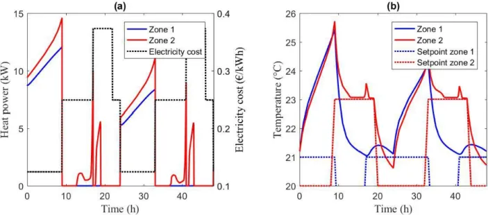
Fig. 3 represents the optimal heating power profiles (a) and the resulting temperature profiles (b) of both zones 1 and 2 achieved with the centralised method. Each zone is pre-heated during off-peak hours to shave off heat consumption during high peak hours, also ensuring that temperature setpoints are respected.
In comparison with the case without demand side management, the total cost was reduced by 22.9 %. For zone 1, 99 % of energy consumption during high peak hours and 100 % of energy consumption during peak hours were reduced. For zone 2, 17 % of energy consumption during high peak hours and 57 % of energy consumption during peak hours were reduced. The minimisation of peak loads is more important for zone 1 (residential space) than for zone 2 (office space). Indeed, the periods when zone 1 needs further heat correspond essentially to off-peak hours unlike zone 2, where further heat needs are exclusively during peak and high peak hours.
Fig. 3. Centralised method results : (a) optimal heating power profiles, (b) resulting temperature profiles.
5.5. Price decomposition-coordination method results
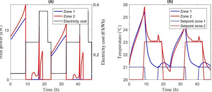
The three decomposition-coordination methods detailed in [14] were implemented in this study. As mentioned above, computations for resource allocation and prediction were too heavy due to the need to provide gradients in local OCPs resolution. The price decomposition-coordination method was preferred. Its results are presented in this section. Fig. 4 represents the optimal heating power profiles (a) and the resulting temperature profiles (b). While local OCPs resolution are done with local dynamic systems (17), resulting temperature profiles were obtained by feeding back optimal heating power profiles into the complete model (2). This procedure allows to confirm that comfort levels are respected. Indeed, Fig. 4 (b) shows that comfort levels are respected even if temperature profiles get closer to the temperature setpoints compared with the centralised method results (Fig. 3 (b)).
In price decomposition-coordination algorithm, the cost was reduced by 22,6 %. For zone 1, 97 % of energy consumption during high peak hours and 100 % of energy consumption during peak hours were reduced. For zone 2, 15 % of energy consumption during high peak hours and 55 % of energy consumption during peak hours were reduced. As for centralised method results, the minimisation of peak loads is more important for zone 1 than for zone 2. Regarding cost and energy reduction, centralised method results are slightly better than decomposition-coordination method results.
Fig. 4. Decomposition-coordination method results : (a) optimal heating power profiles, (b) resulting temperature profiles
6. Conclusion and future work
To conclude, two continuous time resolution methods were performed to find the optimal control of heating in a two-zone building mixing residential and office spaces. The first method applied was the centralised method. This method which consists in solving a unique global OCP converges to the global optimum. To anticipated the increasing complexity of the centralised method at multi-zone scale, a second method called price decomposition-coordination method was applied. Results of the decomposition-coordination method were compared to the global optimum. Regarding cost and energy reduction, results are close even if they are slightly better with the centralised method. With both methods, high peak and peak hours consumptions declined by almost 100 % for zone 1. For zone 2, high peak hours consumption were reduced almost in half nevertheless, peak hours consumption reduction did not exceed 20%.
The decomposition-coordination method presented higher computational time than centralised method. In the experiments, price and wereinitialised to a constant value. Future work
consists in implementing an MPC loop. In this case, prices profiles and can be reused from one OCP resolution to the next one. This is expected to facilitate the decomposition-coordination algorithm convergence and therefore to reduce computational time. Finally the generalisation of both methods to multi-zone buildings is envisaged . Indeed, while computations of centralised method increased exponentially with the number of zones, decomposition-coordination method computational time is expected to increase less dramatically thanks to parallelisation.
Appendix A
This Appendix details the Pontryagin's minimum principle. This principle is a necessary optimality condition asserting that if the control associated to the state is the solution of the OCP then it exists an application called adjoint state which fulfil following assertions:
(29)
(30) (31)
This necessary optimality condition leads to solve the following system of equations:
(32)
Nomenclature
A matrix linking state variation to state B matrix linking state variation to control
C matrix linking state variation to internal and external loads electricity cost,
D matrix linking outputs to state Hamiltonian
p co-state
r augmented Lagrangian parameter s internal and external loads vector, W T indoor temperature, °C
t time, s initial time, s final time, s tol tolerance
u heating power vector, W w interconnection variable x state vector, °C
y outputs vector, °C
Greek symbols
convexity factor of interconnection variable barrier function
penalty factor price
Subscripts and superscripts
i zone number
k decomposition-coordination index max maximal value
min minimal value
References
[1] Robillart M., Etude de stratégies de gestion en temps réel pour des bâtiments énergétiquement performants. Ecole Nationale Supérieure des Mines de Paris 2015.
[2] Expérimenter la construction du bâtiment performant de demain. Ministère de la Cohésion des territoires - Available at <http://www.cohesion-territoires.gouv.fr/experimenter-la-construction-du-batiment-performant-de-demain> [accessed 5.2.2018].
[3] Le saviez-vous ? Ademe - Available at <http://www.ademe.fr/entreprises-monde-agricole/reduire-impacts/maitriser-lenergie-bureaux/dossier/chauffage/saviez> [accessed 5.2.2018].
[4] Les chiffres clés du bâtiment 2011. Ademe - Available at <http://www.envirobat-oc.fr/IMG/pdf/chiffrescles_batiment_2011_ref7487-2.pdf> [accessed 5.2.2018].
[5] Ferreira P.M., Ruano A.E., Silva S., et al., Neural networks based predictive control for thermal comfort and energy savings in public buildings. Energy and Buildings 2012; 55: 238–251.
[6] Marvuglia A., Messineo A., Nicolosi G., Coupling a neural network temperature predictor and a fuzzy logic controller to perform thermal comfort regulation in an office building. Building and Environment 2014; 72: 287–299.
[7] Ma Y., Borrelli F., Hencey B., et al., Model Predictive Control for the Operation of Building Cooling Systems. IEEE Transactions on Control Systems Technology 2012; 20: 796–803. [8] Henze G.P., Kalz D.E., Liu S., et al., Experimental Analysis of Model-Based Predictive
Optimal Control for Active and Passive Building Thermal Storage Inventory. HVACR Research 2005; 11: 189–213.
[9] Moroşan P.D., Bourdais R., Dumur D., et al., A distributed MPC strategy based on Benders’ decomposition applied to multi-source multi-zone temperature regulation. Journal if Process Control 2011; 21: 729–737.
[10] Moroşan P.D., Bourdais R., Dumur D., et al., Building temperature regulation using a distributed model predictive control. Energy and Buildings 2010; 42: 1445–1452.
[11] Lamoudi M.Y., Alamir M., Béguery P., Distributed constrained Model Predictive Control based on bundle method for building energy management. In: 2011 50th IEEE Conference on Decision and Control and European Control Conference. 2011, pp. 8118–8124.
[12] Mesarovic M.D., Macko D., Takahara Y., Two coordination principles and their application in large scale systems control - ScienceDirect. Automatica 1970; 6: 261–270.
[13] Malisani P., Chaplais F., Petit N., An interior penalty method for optimal control problems with state and input constraints of nonlinear systems. Optimal Control Applications and Methods 2014; 37: 3–33.
[14] Carpentier P., Cohen G., Décomposition-coordination en optimisation déterministe et stochastique. Springer, 2017.