How Does Image Content Affect the Added Value of Visual Attention in Objective Image Quality Assessment?

(1)

HAL Id: hal-00788386

https://hal.archives-ouvertes.fr/hal-00788386

Submitted on 14 Feb 2013

HAL is a multi-disciplinary open access

archive for the deposit and dissemination of

sci-entific research documents, whether they are

pub-lished or not. The documents may come from

teaching and research institutions in France or

abroad, or from public or private research centers.

L’archive ouverte pluridisciplinaire HAL, est

destinée au dépôt et à la diffusion de documents

scientifiques de niveau recherche, publiés ou non,

émanant des établissements d’enseignement et de

recherche français ou étrangers, des laboratoires

publics ou privés.

Visual Attention in Objective Image Quality

Assessment?

Hantao Liu, Ulrich Engelke, Junle Wang, Patrick Le Callet, Ingrid

Heynderickx

To cite this version:

Hantao Liu, Ulrich Engelke, Junle Wang, Patrick Le Callet, Ingrid Heynderickx. How Does Image

Content Affect the Added Value of Visual Attention in Objective Image Quality Assessment?. IEEE

Signal Processing Letters, Institute of Electrical and Electronics Engineers, 2013, 20 (4), pp. 355-358.

�10.1109/LSP.2013.2243725�. �hal-00788386�

(2)



Abstract—Our previous research [1] has demonstrated that adding natural scene saliency (NSS) obtained from eye-tracking data may

improve an objective metric’s performance in predicting perceived image quality. In this letter, we further investigate the image content dependency of this improvement. Results show that the variation in saliency between observers highly depends on image content, and that this variation predicts the extent to which a certain image may profit from adding saliency in the objective image quality assessment.

Index Terms—Eye tracking, image quality assessment, objective metric, saliency map, visual attention.

I. INTRODUCTION

dvances in image quality assessment have shown the need and practical attainability of integrating relevant aspects of the human visual system (HVS) in the design of objective quality metrics (OQMs). In the literature, lower level aspects of the HVS, such as contrast sensitivity and masking were successfully modeled and included in various objective metrics [2], [3]. Researchers now attempt to further improve the prediction performance of OQMs by taking into account higher level aspects of the HVS, such as visual attention [4]-[6]. Including visual attention in an OQM is not straightforward yet, basically due to our lack of understanding of how human attention affects the perception of image quality. Two fundamental questions still need to be answered: first, whether visual attention is beneficial for current designs of OQMs, and second, if so, how visual attention should be included in these OQMs.

Literature on the added value of visual attention in OQMs is mainly focused on the extension of an OQM with a (so-called) computational saliency model; a map representing the spatial distribution of image distortions is weighted with the calculated saliency (see, e.g. in [5]). In such an approach, the evaluation of the added value of saliency may heavily depend on the accuracy and reliability of the saliency model used. To

Copyright (c) 2012 IEEE. Personal use of this material is permitted. However, permission to use this material for any other purposes must be obtained from the IEEE by sending a request to pubs-permissions@ieee.org.

Hantao Liu is with the Department of Computer Science, University of Hull, Hull HU6 7RX, United Kingdom. (phone: +44 1482 466534; fax: +44 1482 466666; e-mail: Hantao.Liu@hull.ac.uk).

Ulrich Engelke is with the Group Visual Experiences, Philips Research Laboratories, Eindhoven 5656 AE, The Netherlands. (phone: +31 40 2747855; e-mail: ulrichengelke@gmail.com).

Junle Wang and Patrick Le Callet are with IRCCyN, Ecole Polytechnique de l'Universite de Nantes, Nantes, France. (phone: +33 2 40683047, email: junle.wang@univ-nantes.fr and patrick.lecallet@univ-nantes.fr).

Ingrid Heynderickx is with the Department of Intelligent Systems, Delft University of Technology, Delft 2628 CD, The Netherlands and the Group Visual Experiences, Philips Research Laboratories, Eindhoven 5656 AE, The Netherlands. (phone: +31 40 2747855; fax: +31 40 2744660; e-mail:

How Does Image Content Affect the Added Value of

Visual Attention in Objective Image Quality Assessment?

Hantao Liu, Member, IEEE, Ulrich Engelke, Member, IEEE, Junle Wang, Patrick Le Callet, Member,

IEEE, and Ingrid Heynderickx

(3)

better understand the intrinsic added value of including visual attention in OQMs, researchers used actual visual attention data obtained from eye-tracking recordings (see, e.g. in [6]). In this approach, earlier research [1] demonstrated that addition of natural scene saliency (NSS) was beneficial to prediction performance of OQMs. The results, however, also showed that the actual amount of gain in prediction accuracy depended on several factors, among which were the image content, the distortion type and the objective metric itself. In this letter, we further investigate the image content dependency. Knowledge on this issue may be highly beneficial for the development of a more reliable image quality assessment strategy adaptively incorporating saliency into objective metrics, depending on the visual content.

It has also been demonstrated that the variation in NSS between participants largely depends on the visual content [1]. Hence, in this letter, we first investigate to what extent the variation in NSS between human observers is a reliable measure to classify image content. This evaluation is based on three similar eye-tracking experiments independently conducted in different laboratories. Second, we evaluate whether the extent of such variation indeed affects the actual gain in prediction accuracy that can be obtained by including saliency in objective metrics.

II. VARIATION IN NSS BETWEEN HUMAN OBSERVERS

The eye-tracking data in [1] showed that the variation in NSS between observers strongly depended on the image content. To verify the generalization of this relation we evaluated the similarity in eye-tracking data for three experiments that were conducted independently in different laboratories. With the inter-laboratory comparison we wanted to provide solid evidence on whether the image content determined the variation in NSS between observers, independent of the observer panel and the experimental conditions.

A. Eye-Tracking Experiments

Table 1. Parameters of the setup of the eye-tracking experiments

Eye tracker

Participants

TUD UN UWS

SMI iView X RED (50 Hz) 20 non-experts (12males+8females) 21 non-experts (11males+10females) 15 non-experts (9males+6females) SMI iView X Hi-Speed

(500 Hz)

EyeTech TM3 (45 Hz)

Display _(resolution:19-inch CRT 1024×768) 19-inch LCD (resolution:1280×1024) 19-inch LCD (resolution:1280×1024) Stimuli presentation Viewing distance 10s (+3s mid-gray screen) 15s (+3s mid-gray screen) 12s (+3s mid-gray screen) 60cm 70cm 60cm

In the eye-tracking experiment in [1] (hereafter referred to as TUD), the data of NSS was collected for the twenty-nine source images of the LIVE database [7] by asking human observers to look freely to these images. Similar to TUD, two additional eye-tracking experiments were performed: one in a laboratory at the University of Nantes, France (hereafter referred to as UN) [8], and the other one in a laboratory at the University of Western Sydney, Australia (hereafter referred to as UWS) [9]. The three experiments were not conducted jointly for the purpose of comparison, but rather were carried out independently using well-calibrated equipment and a well-defined experimental protocol with the aim to find “ground truth” saliency data. Some important parameters for each experimental setup are listed in Table 1.

B. Variation in Saliency among Individuals

(4)

constructed adding to each fixation location a Gaussian patch, which approximates the size of the fovea in the human eye (about 2 of visual angle, corresponding to a σ of 45 pixels for the Gaussian for all three experiments). The intensity of the resulting saliency map ranges from 0 to 1. In this letter, two types of SM are generated: one in which the mean saliency is calculated over all fixations of all subjects (MSM), and a second one, in which saliency is calculated with the fixations of an individual subject only (ISM). The variation in NSS between human observers is then quantified as the correlation coefficient ρ (with its value ranging between [-1, 1]) between the MSM and each ISM, averaged over all participants. Note that alternative measures to compare saliency maps exist (e.g., receiver operating characteristics (ROC)), but since conclusions tend to be consistent over these measures [10], we decided to focus on the correlation coefficient only. The averaged ρ-value provides a quantitative correspondence in saliency between observers: a large value indicates a small variation in saliency among participants, while a small value indicates that the saliency is widely spread among subjects.

0.4 0.5 0.6 0.7 0.8 0.9 1 2 3 4 5 6 7 8 9 10 11 12 13 14 15 16 17 18 19 20 21 22 23 24 25 26 27 28 29 TUD UN UWS ρ-value image

Fig. 1. Correlation coefficient (ρ-value) between the MSM and the ISM averaged over all subjects per image, for the eye-tracking data of TUD, UN, and UWS, respectively. The vertical axis indicates the averaged ρ-value, and the horizontal axis indicates the twenty-nine images of the LIVE database (the standard deviation of ρ is 0.06 for TUD, UN and UWS).

Figure 1 illustrates the averaged ρ-values for the twenty-nine images of the LIVE database, determined from the three eye-tracking experiments respectively. It clearly shows that the averaged ρ-value strongly varies over the different scenes in each experiment; the difference between the highest and lowest value of ρ is 0.30 for TUD, 0.25 for UN and 0.25 for UWS. To evaluate whether the scene dependency of ρ is equal over the three laboratories, and thus independent of the choice of observers and of the experimental conditions, the ρ-values of the 29 images are first ranked in descending order for each laboratory independently. This results in an entity R containing three elements per image:

R(image) = [rank_TUD, rank_UN, rank_UWS] (1)

where rank_TUD, rank_UN, and rank_UWS are the actual ranks of the ρ-value per image for TUD, UN and UWS respectively. Figure 2 (a) illustrates the three-dimensional scatter plot of the entity R for the 29 images. This plot visualizes the consistency of the ranking of images between different experiments; the shorter the distance of a marker (i.e. an image) to the space diagonal is, the more consistent are the ranks among the three laboratories for that image. In general, all images are spread around the 3-D diagonal in a rather compact manner (this trend is also visualized with 2-D plots in Figure 2(b)), suggesting that saliency is determined to a great extent by the content of the image rather than by differences in individuals or by small differences in experimental conditions.

(5)

0 510 15 2025 30 0 5 10 15 20 25 30 0 5 10 15 20 25 30 TUD UN U W S (a) 0 5 10 15 20 25 30 0 5 10 15 20 25 30 UWS TUD 0 5 10 15 20 25 30 0 5 10 15 20 25 30 UWS UN (b)

Fig. 2. (a) The three-dimensional scatter plot of the ranks of the 29 images in the three eye-tracking experiments, i.e. TUD, UN, and UWS. Each green marker indicates one individual image, and the red line indicates the space diagonal. (b) The 2-D scatter plots showing one example of the two combinations of (a), i.e. TUD vs. UWS and UN vs. UWS. The red lines correspond to linear fitting for the data points.

C. Saliency-based Content Classification

Fig. 3. Saliency-based (i.e., on the ρ-value) image classification for the 29 source images of the LIVE database: six images had a high value of ρ in each of the three eye-tracking experiments, four images had a low value of ρ in each of the experiments, and the remaining nineteen images were classified to the category of medium ρ-value.

The inter-laboratory comparison demonstrates that the image content strongly, if not completely, determines the extent of variation in saliency between observers. This essentially makes the classification of image content based on the ρ-value rather meaningful. In Figure 2 (a), image clustering patterns are clearly observed: (1) six images are located extremely closely to the space diagonal in the region of high ρ-values (i.e. from rank 1 to 6 with a ρ-value higher than 0.7), (2) four images are placed very closely to the space diagonal in the region of low ρ-values (i.e. from rank 26 to 29 with a ρ-value lower than 0.63), and (3) the remaining nineteen images with a medium ρ-value are spread around the space diagonal. This implies that the three eye-tracking experiments mainly share a high agreement in saliency for images with a high or low consistency in saliency between individuals.

To check the resulting classification on the LIVE database, the images with a high, medium or low ρ-value are visualized in Figure 3. The images yielding the six highest ρ-values in each of the three eye-tracking experiments generally contain a few salient features, such as faces or texts; the saliency converges around these features for each participant. The images with the four lowest ρ-values in each of the experiments clearly lack highly salient features, with the consequence that the saliency is randomly distributed over the whole image for the different subjects.

(6)

III. THE EFFECT OF CONTENT DEPENDENCY ON OBJECTIVE IMAGE QUALITY METRICS

Research in [1] has demonstrated that including NSS obtained from eye-tracking data into several well-known OQMs in general improves the metric’s prediction performance over the performance of the same metric without saliency. This conclusion was drawn based on an evaluation over the entire LIVE database, including a variety of distortion types (i.e., JPEG compression (JPEG), JPEG2000 compression (JP2K), white noise (WN), Gaussian blur (GBLUR), and simulated fast-fading Rayleigh occurring in (wireless) channels (FF)). To further investigate the image content dependency in the performance gain of adding saliency to OQMs, we repeated the experiment in [1] (again using the NSS of TUD) for the source images classified as “low”, “medium” and “high” ρ-value, respectively (i.e. by taking into account the extent of variation in saliency between individuals). The number of stimuli for each category and for each distortion type provided by the LIVE database is listed in Table 2.

Table 2. Number of stimuli for each category of saliency-based image classification and for each distortion type as provided by the LIVE database JPEG JP2K WN GBLUR FF

TOTAL 233 227 174 174 174

Low ρ-value 34 31 24 24 24 Med. ρ-value 151 149 114 114 114 High ρ-value 48 47 36 36 36

For practical reasons, the objective metrics used in our evaluation are limited to three metrics that are so far widely accepted in the image quality community: PSNR (peak signal-to-noise ratio [2]), SSIM (structural similarity index [2]) and VIF (visual information fidelity [2]). Locally weighting (i.e. by multiplication) the distortion maps of these metrics with the NSS map results in three saliency-based metrics, which are referred to as WPSNR, WSSIM, and WVIF. The performance of a metric is quantified by the Pearson linear correlation coefficient (CC) indicating prediction accuracy, the Spearman rank order correlation coefficient (SROCC) indicating prediction monotonicity, and the root-mean-squared error (RMSE), between the subjective scores (i.e., DMOS) and the metric’s predictions.

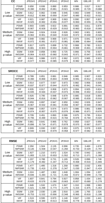
Table 3 illustrates the comparison in performance gain between a metric and its saliency-based version averaged over all distortion types and for the images of “low”, “medium” and “high” ρ-value separately. The overall gain (averaged over distortion type where appropriate) of an saliency-based metric over its corresponding metric without NSS is summarized in Table 4. Both tables demonstrate that the actual gain in prediction performance that can be obtained by including saliency in objective metrics is largely affected by the ρ-value, independent of the metric used and of the image distortion type tested. In general, it shows the consistent trend that the amount of performance gain increases as the ρ-value increases. The rate of increase (i.e. from “low” to “medium” ρ-value or from “medium” to “high” ρ-value), however, depends on the metric and on the distortion type. The increase in performance gain as a consequence of the increase of ρ-value is not obvious for the subset of the LIVE database distorted by WN (compared to other distortion types, see Table 3), and also is not obvious for the VIF metric (compared to other two metrics, see Table 4). Differences in the rate of increase in performance gain may be attributed to the fact that the performance of a metric (i.e., without NSS) varies with the distortion type, and the overall performance differs for different metrics. As such, it is more difficult to obtain a significant increase in performance by adding NSS when a high prediction performance is already achieved with a metric (e.g., a high performance is found for all three metrics applied to WN, and the overall performance of VIF is already high). Such relatively small performance

(7)

gains possibly mask the rate of increase.

Table 3. Comparison in performance gain (quantified by CC, SROCC and RMSE) between a metric and its saliency-based version (PSNR versus WPSNR, or SSIM versus WSSIM, or VIF versus WVIF) separately for the image sets of “low”, “medium” and “high” ρ-value from the LIVE database.

JPEG#1 JPEG#2 JP2K#1 JP2K#2 WN GBLUR FF

0.650 /0.390 0.936 /0.892 0.953 /0.921 0.817 /0.729 0.917 /0.888 0.880 /0.861 0.986 /0.985 PSNR /WPSNR 0.944 /0.962 0.924 /0.951 0.918 /0.940 0.926 /0.943 0.963 /0.972 0.901 /0.930 0.903 /0.926 0.941 /0.977 0.986 /0.994 0.962 /0.979 0.972 /0.982 0.965 /0.984 0.923 /0.940 0.972 /0.985 0.921 /0.925 0.969 /0.956 0.963 /0.977 0.987 /0.992 0.990 /0.993 0.957 /0.955 0.807 /0.796 VIF /WVIF 0.812 /0.812 0.962 /0.966 0.948 /0.959 0.945 /0.947 0.983 /0.980 0.949 /0.922 0.941 /0.921 SSIM /WSSIM 0.870 /0.903 0.968 /0.969 0.899 /0.904 0.732 /0.861 0.817 /0.881 0.780 /0.801 0.913 /0.909 0.811 /0.818 0.922 /0.929 0.903 /0.907 0.905 /0.928 0.983 /0.983 0.879 /0.900 0.891 /0.910 Medium p-value 0.949 /0.972 0.971 /0.981 0.976 /0.988 0.941 /0.964 0.879 /0.889 0.982 /0.991 0.969 /0.972 High p-value Low p-value PSNR /WPSNR PSNR /WPSNR SSIM /WSSIM SSIM /WSSIM VIF /WVIF VIF /WVIF CC 0.858 /0.925 0.966 /0.971 0.950 /0.960 0.725 /0.843 0.939 /0.964 0.756 /0.947 0.927 /0.953

0.789 /0.390 0.851 /0.868 0.946 /0.909 0.907 /0.812 0.920 /0.923 0.881 /0.804 0.985 /0.991 PSNR /WPSNR 0.959 /0.967 0.897 /0.932 0.947 /0.961 0.950 /0.956 0.962 /0.967 0.926 /0.940 0.947 /0.963 0.909 /0.940 0.930 /0.948 0.953 /0.958 0.975 /0.977 0.978 /0.982 0.926 /0.931 0.957 /0.979 0.935 /0.935 0.958 /0.937 0.973 /0.973 0.917 /0.930 0.994 /0.996 0.925 /0.902 0.824 /0.824 VIF /WVIF 0.914 /0.837 0.877 /0.877 0.937 /0.944 0.973 /0.973 0.982 /0.982 0.956 /0.941 0.935 /0.941 SSIM /WSSIM 0.451 /0.499 0.975 /0.976 0.893 /0.915 0.586 /0.784 0.709 /0.795 0.795 /0.794 0.914 /0.920 Medium p-value 0.968 /0.974 0.973 /0.976 0.986 /0.986 0.961 /0.971 0.868 /0.876 0.957 /0.957 0.974 /0.975 High p-value Low p-value PSNR /WPSNR PSNR /WPSNR SSIM /WSSIM SSIM /WSSIM VIF /WVIF VIF /WVIF SROCC 0.641 /0.734 0.958 /0.970 0.965 /0.971 0.762 /0.878 0.861 /0.896 0.827 /0.967 0.959 /0.977 0.926 /0.944 0.795 /0.816 0.879 /0.907 0.818 /0.830 0.893 /0.916 0.948 /0.962 0.985 /0.985

2.350 /3.145 1.504 /1.938 0.996 /1.260 3.460 /3.329 1.678 /1.797 2.135 /2.047 0.735 /0.733 PSNR /WPSNR 1.024 /0.846 1.487 /1.283 1.902 /1.721 1.648 /1.456 1.084 /0.872 1.094 /0.999 1.937 /1.739 1.519 /0.636 0.595 /0.389 1.140 /0.666 0.847 /0.778 1.030 /0.459 1.441 /1.083 0.973 /0.613 1.207 /1.179 0.731 /1.347 1.165 /0.713 0.788 /0.482 0.526 /0.468 0.896 /0.916 1.748 /1.806 VIF /WVIF 1.927 /1.955 1.210 /1.215 0.972 /0.933 1.524 /1.552 0.700 /0.713 0.942 /1.071 1.092 /1.306 SSIM /WSSIM 1.532 /1.298 1.310 /1.315 1.673 /1.774 1.947 /1.370 1.949 /1.621 1.998 /1.875 1.583 /1.453 2.032 /1.847 1.318 /1.378 1.477 /1.735 1.495 /1.419 0.980 /1.030 1.456 /1.424 1.358 /1.347 Medium p-value 1.607 /0.633 0.927 /0.663 0.958 /0.657 1.434 /0.680 1.641 /1.278 0.841 /0.578 0.794 /1.090 1.230 /0.753 2.030 /1.532 1.185 /0.906 2.916 /2.348 1.166 /0.965 1.765 /0.818 1.526 /1.186 High p-value Low p-value PSNR /WPSNR PSNR /WPSNR SSIM /WSSIM SSIM /WSSIM VIF /WVIF VIF /WVIF RMSE

To also check whether the numerical difference in performance between a metric with NSS and the same metric without NSS is statistically significant, hypothesis testing is conducted. The test is based on the residuals between the DMOS and the quality predicted by the metric (referred to as M-DMOS residuals). A paired-sample t-test is used to test the statistical significance for the difference between the two sets of M-DMOS residuals (i.e. one from the metric itself and one from the same metric after adding the NSS). The paired-sample t-test starts from the null hypothesis stating that the residuals of one metric are statistically indistinguishable (with 95% confidence) from the residuals of that same metric with NSS. The results of this t-test are given in Table 5 for all metrics and distortion types separately. This table illustrates that in most cases the difference in prediction performance by adding NSS to an objective metric is statistically significant. For the condition of “medium” ρ-value, all

(8)

combinations of metrics applied to all given distortion types were tested statistically significant. It should, however, be noted that the outcome of statistical significance testing largely depends on the number of sample points, which is limited for the conditions “low” ρ-value and “high” ρ-value (see Table 2).

Table 4. Performance gain between a metric and its saliency-based version averaged over all distortion types for the image sets of “low”, “medium” and “high” ρ-value from the LIVE database

CC SROCC CC SROCC CC SROCC

RMSE RMSE RMSE

0.20 0 -0.18 0.05 -0.18 -0.47 -0.02 -0.37 -0.42

Table 5. Results of t-test based on M-DMOS residuals: “1” means that the difference in performance between the metric with NSS and the same metric without NSS is statistically significant, and “0” means that the difference is not statistically significant

Low p-value Medium p-value High p-value PSNR and WPSNR PSNR and WPSNR PSNR and WPSNR SSIM and WSSIM

SSIM and WSSIM

SSIM and WSSIM VIF and WVIF

VIF and WVIF

1 1 1 1 1 1 1 1 1 1 1 1 1 1 1 1 1 1 1 1 1 1 1 1 1 1 1 1 1 1 1 1 1 1 1 1 1 1 1 1 1 1 1 1 0 0 0 0 0 0 0 0 0 0 0 0 0 0 0 0 0 0 0

Figure 4 plots the performance gain of the objective metrics when saliency is added for the different ranges of ρ-value, i.e. for the “low”, “medium” and “high” image sets. It shows that for a ρ-value above 0.63 adding saliency is beneficial to improve the quality prediction performance of the objective metrics PSNR, SSIM and VIF. For the images of “low ρ-value” (i.e. ρϵ[0.45, 0.6]), the performance gain when adding saliency is either non-existing or even negative. No change in performance when adding saliency can be expected for images, for which the saliency is uniformly spread over the entire image; including saliency to a metric then does not make any difference with averaging the metric over the whole image without weighting. A decrease in prediction performance by adding saliency can occur when the randomly distributed saliency coincidentally gives more weight to non-distorted regions than to heavily distorted regions in an image. For the images of “medium ρ-value” (i.e. ρϵ[0.63, 0.72]) and “high ρ-value” (i.e. ρϵ[0.73, 0.76]) the performance gain is always positive, and adding saliency results in a larger gain for the images of “high ρ-value” than for the images of “medium ρ-value”. As illustrated in Table 4, the gain in performance when adding saliency is twice as high for the images of “high ρ-value” than for the images of “medium ρ-value”.

-0.08 -0.06 -0.04 -0.02 0 0.02 0.04 0.06 0.08 [0.45, 0.6] [0.63, 0.72] [0.73, 0.76] PSNR SSIM VIF ρ-value CC

(9)

of ρ-value for the image sets of “low”, “medium” and “high” ρ-value from the LIVE database, respectively.

IV. CONCLUSIONS AND FUTURE DIRECTIONS

In this letter, based on eye-tracking data, we found out that the extent of variation in visual saliency between observers is strongly image content dependent. The smaller the variation in saliency, i.e. the more convergent the saliency map, the larger the actual performance gain that can be obtained by including saliency in objective metrics. For the images having a large variation in saliency, adding saliency to a metric runs the risk of degrading the performance of the metric for quality prediction. For the PSNR, SSIM and VIF metrics, we found a threshold value in ρ of 0.63, above which including saliency is beneficial for objective quality prediction.

Our new findings are valuable to guide developers or users of image quality metrics to decide, based on their own application environment, whether or not to include saliency. Of course, calculating a ρ-value in order to decide whether or not to include saliency is unrealistic in any application context. But, since this letter illustrates that the ρ-value is linked to the spread in the saliency map, this spread may be used as an alternative decision criterion, i.e., saliency should only be applied in case this spread is low. More research needs to be done to exactly formulate the criterion in terms of spread in the (modeled) saliency map, and as such, make the criterion practically applicable. Recently, we found that adaptively incorporating saliency, based on image content, indeed is promising in image quality prediction [11].

In addition, one should take into account the performance of a metric without saliency, since this letter illustrates that the performance gain is limited in case the metric without saliency already has a good performance (e.g., VIF). For those metrics, computational power can be reduced by avoiding the computation of saliency. This, in a way, also implies that the additional computational cost to include saliency may as well be used to improve the basic objective metrics’ performance.

REFERENCES

[1] H. Liu and I. Heynderickx, “Visual Attention in Objective Image Quality Assessment: based on Eye-Tracking Data,” IEEE Trans. CSVT, vol. 21, pp. 971-982, July, 2011.

[2] Z. Wang and A. C. Bovik, Modern Image Quality Assessment (Synthesis Lectures on Image, Video and Multimedia Processing). San Rafael, CA: Morgan and Claypool, 2006.

[3] H. Liu, Modeling Perceived Quality for Imaging Applications. PhD Thesis, Delft University of Technology, The Netherlands, 2011.

[4] U. Engelke, H. Kaprykowsky; H.-J. Zepernick and P. Ndjiki-Nya; “Visual Attention in Quality Assessment,” vol. 6, pp. 50-59, IEEE Signal Processing Magazine, 2012.

[5] J. You, A. Perkis, M. Hannuksela and M. Gabbouj, “Perceptual quality assessment based on visual attention analysis,” in Proc. ACM Multimedia 2009. [6] O. Le Meur, A. Ninassi, P. Le Callet, and D. Barba, “Overt visual attention for free-viewing and quality assessment tasks: Impact of the regions of interest on

a video quality metric,” Signal Process. Image Communication, vol. 25, no. 7, pp.547-558, 2010.

[7] H. R. Sheikh, Z. Wang, L. Cormack, and A. C. Bovik. LIVE Image Quality Assessment Database Release 2 [Online]. Available: http://live.ece.utexas.edu/research/quality

[8] J. Wang, R. Pepion, and P. Le Callet, “IRCCyN/IVC eyetracker images LIVE database,” http://www.irccyn.ecnantes.fr/, 2011.

(10)

[10] U. Engelke, H. Liu, J. Wang, P. Le Callet, I. Heynderickx, H. Zepernick and A. Maeder, “A comparative Study of Fixation Density Maps,” IEEE Trans. Image Processing, in press.