HAL Id: hal-01096588
https://hal.archives-ouvertes.fr/hal-01096588
Submitted on 19 Dec 2014HAL is a multi-disciplinary open access archive for the deposit and dissemination of sci-entific research documents, whether they are pub-lished or not. The documents may come from teaching and research institutions in France or abroad, or from public or private research centers.
L’archive ouverte pluridisciplinaire HAL, est destinée au dépôt et à la diffusion de documents scientifiques de niveau recherche, publiés ou non, émanant des établissements d’enseignement et de recherche français ou étrangers, des laboratoires publics ou privés.
A Method for the Rapid Generation of Nonsequential
Light-Response Curves of Chlorophyll Fluorescence
Joao Serôdio, Joao Ezequiel, Jörg Frommlet, Martin Laviale, Johann Lavaud
To cite this version:
Joao Serôdio, Joao Ezequiel, Jörg Frommlet, Martin Laviale, Johann Lavaud. A Method for the Rapid Generation of Nonsequential Light-Response Curves of Chlorophyll Fluorescence. Plant Phys-iology, American Society of Plant Biologists, 2013, 163, pp.1089-1102. �10.1104/pp.113.225243�. �hal-01096588�
1 Running Head: Single pulse light curves
1 2 3 João Serôdio 4 5
Departamento de Biologia and CESAM – Centro de Estudos do Ambiente e do Mar, 6
Universidade de Aveiro, Campus de Santiago, 3810-193 Aveiro, Portugal 7 Tel: +351 234370787 8 E-mail: jserodio@ua.pt 9 10
Research area: Breakthrough Technologies 11
2 A method for the rapid generation of non-sequential light-response curves of chlorophyll 13 fluorescence 14 15 16 17 18 19 20
João Serôdio1, João Ezequiel1, Jörg Frommlet1, Martin Laviale1, Johann Lavaud2 21
22
Address: 1Departamento de Biologia and CESAM – Centro de Estudos do Ambiente e do Mar, 23
Universidade de Aveiro, Campus de Santiago, 3810-193 Aveiro, Portugal; 2UMR 7266 24
‘LIENSs’, CNRS-University of La Rochelle, Institute for Coastal and EnvironmentalResearch 25
(ILE), 2 rue Olympe de Gouges, 17 000 La Rochelle, France 26
27 28 29
One-sentence summary: Light-response curves of chlorophyll fluorescence are rapidly 30
generated from independent, non-sequential measurements through the combined use of 31
spatially separated beams of actinic light and fluorescence imaging. 32
3 Financial source: This work was supported by the FCT – Fundaçãopara a Ciência e a
34
Tecnologia, through grants SFRH/BSAB/962/2009 (J.Serôdio), SFRH/BD/44860/2008 (J. 35
Ezequiel), and projectsMigROS (PTDC/MAR/112473/2009; M. Laviale),SeReZoox 36
(PTDC/MAR/113962/2009; J. Frommlet), by the CNRS – Centre National de la 37
RechercheScientifique (‘chercheursinvités’ program, J. Serôdio and J.Lavaud), and by the 38
French consortium CPER-Littoral, and the Egide/Campus France PHC Pessoa exchange 39
program (n°27377TB to J. Serôdio and J. Lavaud ). 40
41
Corresponding author: João Serôdio, jserodio@ua.pt 42
4 Abstract
44
Light-response curves (LC) of chlorophyll fluorescenceare widely used in plant physiology. 45
Most commonly, LCs are generated sequentially,exposing the same sample to a sequence of 46
distinct actinic lightintensities. These measurements are not independent, as the response to 47
each new light level is affected by the light exposure history experienced during previous steps 48
of the LC, an issue particularly relevant in the case of the popular Rapid Light Curves.In this 49
work we demonstrate the proof of concept of a new method for the rapid generation of LCs 50
from non-sequential, temporally-independent fluorescence measurements. The method is based 51
on the combined use of sample illumination with digitally controlled, spatially separated beams 52
of actinic light, andof a fluorescence imaging system. It allows the generationof a whole LC, 53
including a large number of actinic light steps and adequate replication, within the time required 54
for a single measurement (therefore named ‘Single Pulse Light Curve’). This method is 55
illustrated for the generation of LCs of PSII quantum yield (∆F/Fm'), relative electron transport
56
rate (rETR) and non-photochemical quenching (NPQ), on intact plant leavesexhibiting distinct 57
light responses. This approach makes it also possible to easily characterize the integrated 58
dynamic light response of a sample, by combining the measurement of LCs (actinic light 59
intensity is varied while measuring time is fixed) with induction/relaxation kinetics (actinic light 60
intensity is fixed and the response is followed over time), describing both how the response to 61
light varies with time and how the response kinetics varies with light intensity. 62
5 Light-response curves (LC) are widely used in plant physiology for the
64
quantitativedescriptionof the light-dependence of photosynthetic processes (Henley, 1993). 65
Originally developed for characterizing the response of steady state photosynthesis to ambient 66
irradiance (Smith, 1936), LCs attained widespread use following the introduction of Pulse 67
Amplitude Modulated (PAM) fluorometry (Schreiber et al., 1986). Through its ability to 68
monitor the activity of photosystem II (PSII), this technique allows the generation of LCs of 69
relative electron transport rate (rETR;Schreiber et al., 1994), a non-invasive and real-time 70
indicator of photosynthetic activity, shown to be a close proxy for biomass-specific rates of 71
photosynthesis (Genty et al., 1989; Seaton and Walker, 1990). Due to the considerable 72
operational advantages of PAM fluorometry, LCs of rETR became the most common form of 73
quantitatively characterize the light response of photosynthetic activity in plants as well as in 74
virtually all types of photoautotrophic organisms (Rascher et al., 2000; Serôdio et al., 2005; Ye 75
et al., 2012). 76
Ideally, LCs should be based on independent measurements of the parameter under study. 77
For example, in 14C-based methods of measuring photosynthetic rates in phytoplankton this is 78
the case (Johnson and Sheldon, 2007). It is also possible to generate LCs from PAM 79
measurements in independent replicated samples (Lavaud et al., 2007) but the need to cover a 80
wide range of actinic light levels with appropriate replication makes this approach very time and 81
sample consuming. Therefore, in most cases LCs are generated sequentially, by exposing the 82
same sample to a (usually increasing) range of irradiance levels (Schreiber et al., 1994). 83
An often overlooked consequence of sequential LCsis that the response of the sample 84
under each light level is strongly affected by its exposure to previous light levels (Perkins et al., 85
2006; Herlory et al., 2007; Ihnken et al., 2010). LCs constructed in this way are therefore 86
dependent not only on the absolute light levels applied during the generation of the curve but 87
also on the duration of the exposure to each light level and on their order of application. The 88
effects of non-independency between measurements are expected to be intensified in the case of 89
rapid light curves (RLC; Schreiber et al., 1997; White and Critchley, 1999), curves generated by 90
reducing the duration of each light step, normally to just 10-30 s (Rascher et al., 2000; Ralph 91
and Gademann, 2005; Perkins et al., 2006). The short duration of the light steps do not allow the 92
sample to reach a steady state under each light level, thus being largely influenced by previous 93
light history(Serôdio et al., 2006; Ihnken et al., 2010; Lefebvre et al., 2011). 94
Here we present an alternative method to generateLCs of fluorescence parameters from 95
truly independent, non-sequential measurements. The method is based on the spatial separation 96
of the different levels of actinic light used to construct the light curve, and uses the capabilities 97
of chlorophyll fluorescence imaging systems to simultaneously measure the fluorescence 98
emitted by samples exposed to different irradiance levels. This approach enables light curves to 99
be measured very rapidly, as it only requires that the samples are exposed to the different actinic 100
6 light levels for the desired period of time (e.g. to reach a steady-state condition) before a single 101
saturating pulse is applied to measure the fluorescence response of all samples simultaneously. 102
By reducing significantly the time required for the generation of LCs, this approach makes it 103
possible to easily characterize the dynamic light response, by simultaneously tracing the 104
fluorescence response under different light intensities over time. 105
This work demonstrates the proof of concept for the generation of LCs through the 106
combined use of (i) sample illumination with spatially separated light beams of different 107
intensity, through the use a digital projector as a source of actinic light, and (ii) 108
imagingchlorophyll fluorometry. The application of the method is illustrated for intact plant 109
leaves, but its general principle of operation is applicable to any other type of photosynthetic 110
samples, like macroalgae, lichens or suspensions of microalgae or chloroplasts. 111 112 113 RESULTS 114 115
Rationale of the method 116
The method is based on the illumination of replicated samples with actinic light of different 117
intensities and on the simultaneous detection of the induced fluorescence by an imaging 118
chlorophyll fluorometer. The method requires a number of conditions to be met. 119
A fundamental requirement is that the illumination of the samples with different levels of 120
actinic light must not interfere with its exposure to the measuring light and saturation pulses. 121
For this reason, the best solution is to project on the samples the required combination of actinic 122
light levels (‘light mask’, see below) using a light source positioned from such a distance that 123
the measuring light and saturating pulses can reach the samples unimpeded. This approach also 124
allows for the measuring light and the saturating pulses to illuminate the sample while it is 125
exposed to the actinic light, a critical condition of the saturating pulse method (Schreiber et al., 126
1986). Nonetheless, in order to be useful for the generation of a light curve, the fluorescence 127
response must be related solely to the different actinic light levels applied. This implies the use 128
of either replicated samples (e.g. microalgae culture in a multi-well plate) or a homogeneous 129
single sample (e.g. whole leaf). In the latter case, however, the independence of the 130
measurements may be compromised by light scattering within the sample (leaf tissue) causing 131
light spillover between adjacent areas illuminated with different actinic light levels (see below). 132
In this study a digital projector was used as a source of actinic light, due to the large potential 133
advantages deriving from the versatility provided by the digital control of light output. 134
However, the novelty of this approach in plant photophysiology required extensive testing both 135
regarding the emitted light and the detection of fluorescence response. 136
7 Regarding light output, the digital projector used in this study was analyzed concerning 137
the spectral characteristics of the emitted light. An important condition for any light source to be 138
used for generating light-response curves is that the light spectrum does not change significantly 139
over the range of light intensities applied. Otherwise, substantial distortions in the light curve 140
shape may be induced, as the photosynthetic light absorption varies significantly along the 141
different regions of the spectrum. This was tested by measuring the spectrum of light emitted at 142
the various output intensities used for generating light curves. 143
The use of a digital projector was also tested regarding the potential interference on the 144
detection of the fluorescence signals. Images produced by digital projectors are known to suffer 145
from flickering which, although imperceptible to the human eye, may affect the determination 146
of fluorescence levels Fs and Fm’ and the calculation of fluorescence indices like ∆F/Fm’ or
147
NPQ. Preliminary tests were made on the two main types of digital projector, LCD and DLP 148
projectors. In LCD projectors, images are generated from light beams (three, each of one 149
primary color) passing through separate LCD panels made of a large number of liquid crystals, 150
each corresponding to a pixel in the projected image. The three beams are later combined into a 151
single, full color beam. In the case of DLP technology, the projected light beam arises from 152
light reflected from a reflective surface made of a large number of small mirrors (DLP chip), 153
each corresponding to a pixel in the final image. The orientation of each mirror is controlled 154
individually determining the intensity of each pixel. The interference of actinic light flickering 155
on fluorescence measurements was tested by analyzing the fluorescence kinetics immediately 156
before (determination of Fs level) and during the application of a saturating pulse (determination
157
of Fm’ level), on samples exposed to different actinic light intensities provided by the projector.
158
DLP projectors exhibited a much higher intensity of flickering, making them impossible to use 159
in this context. The study was thus carried out using a LCD projector (see below). 160
161
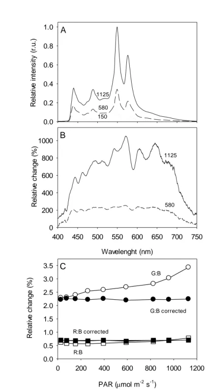
Actinic light spectrum 162
The spectrum of the light emitted by the digital projector covered the wavelength range of 163
PAR, from ca. 430 nm to over 700 nm (Fig. 2A). The projected light was rich in 164
photosynthetically active blue light, its spectrum showing a distinct peak at 440 nm, but poorer 165
in red light (650-700 nm band). The spectrum showed two large peaks in the green-yellow 166
region, centered at 550 and 580 nm. Very little thermal radiation (above 750 nm) was emitted, 167
even when applying the highest PAR levels. This means that the used projectorwas a suitable 168
source of coldactinic light, which did not induce differences in temperature over the different 169
AALs. 170
The light spectrum was found to change substantially when varying the lamp output 171
intensity (Fig. 2B). Below moderate PAR values (e.g. 580 µmol m-2 s-1 at the sample level), 172
irradiance increased equally over most of the spectral range (flat spectrum from 440 to 675 nm; 173
8 when compared to 150 µmol m-2 s-1). But for higher lamp outputs (e.g. 1125 µmol m-2 s-1), the 174
spectrum was increasingly enriched in green-yellow light (mainly green, 525-590 nm, and 175
yellow-orange, 600-660 nm) becoming comparatively poorer in photosynthetically active blue 176
and red light. The variation of the light spectrum with intensity may represent a major problem 177
for the generation of light-response curves. Because the yellow-green light that dominates the 178
spectrum when applying higher light levelsis poorly absorbed by photosynthetic pigments, the 179
corresponding values of ∆F/Fm’ (or rETR) will appear overestimated when plotted against the
180
measured PAR levels. As a result, rETRlight-response curves may show an inflexion in the 181
light-saturated region, showing an increase of rETR values when stabilizationor even a decrease 182
would be expected. 183
This problem was addressed by manipulating the spectrum of emitted light so that the 184
proportions of red, green and blue (RGB ratio) regions of the spectrum remained approximately 185
constant over the whole range of light intensities applied.This was achieved through an iterative 186
process of changing the MS Visual Basiccode controlling the RGB ratio of the images produced 187
by the projector, measuringthe emitted spectrum, and calculatingthe resulting proportions of 188
red, green and blue spectral regions. The RGB code allowed to independently controlthe 189
spectral ranges of 400-486 (blue), 487-589 (green-yellow) and 590-690 (red) nm.This procedure 190
was repeated until the same proportions of RGB were obtained in the emitted light for the 191
various PAR levels that were used for generating light-response curves.An average proportion 192
R:G:B of 0.7:2.2:1was used (Fig. 2C), which,by having a higher proportion of yellow-green 193
light ensured the emission of high maximum PAR levels (1125 µmol m-2 s-1 at the sample 194
level). 195
196
Actinic light flickering 197
The projector light showed noticeable flickering, causing obvious fluctuations in the 198
fluorescence trace (Fig. 3). Light flickering caused interferences at 1.8 s intervals, more 199
pronounced under higher actinic light levels, when it significantly affected the correct 200
determination of both Fs and Fm’ levels.Using the data of Fig. 3 as an example, if the full
201
fluorescence record was considered for calculating Fs and Fm’, it would result in an
202
underestimation of ∆F/Fm’ values of 3.0% and 22.3%, for 260 and 850 µmol m -2
s-1, 203
respectively. To avoid these confounding effects it was necessary to analyze the fluorescence 204
recording for each individual measurement (immediately before and during a saturating pulse) 205
and exclude the affected data points. 206
207
Application to intact leaves 208
The method was tested on intact leaves of plants acclimated to different light regimes, 209
expected to show contrasting features in light-response curves of fluorescence. Figure 4 shows 210
9 chlorophyll fluorescence images resulting from the application of anactinic light mask to leaves 211
of HL-acclimated Hedera helix (Fig. 4A-C) and LL-acclimated Ficusbenjamina (Fig. 4D-F)for 212
a known period of time. 213
Images of Fs andFm’ of H. helix(Fig.4A,B) showed some degree of heterogeneity, with
214
higher absolute pixel values in the central region of the leaf, and lower values in the extremities. 215
This was due to the large leaf size in relation to the projected light fieldsof measuring light and 216
saturating pulses. However, this didnot affect significantly the determination of the ratio 217
∆F/Fm’, which remainedrelatively constant throughout the whole leaf (varying between 0.79
218
and 0.83; Fig. 4C). In the case of F. benjamina, although the smaller leaf size helped reduce the 219
effects of light field heterogeneity,spatial variability was still noticeable due to certain leaf 220
anatomical features (e.g. central vein). Again, while this was evident for Fs and Fm’ images, the
221
effect mostly disappeared when the ratio ∆F/Fm’ was calculated (Fig. 4F).
222
The application of the actinic light maskon intact leaves resulted in well-defined areasof 223
induced fluorescence response. Particularly for higher light levels, each AAL showed a 224
noticeable outer ring of pixels of intensity intermediate between background values (not 225
illuminated areas) and fully illuminated areas (center of each AAL). The resulting fluorescence 226
images showed a clearly different pattern of response to actinic light in the two plants. Whilst 227
for the HL-acclimated H. helix, little effects were observed on Fs, which remained virtually
228
constant over the range of PAR levels applied (Fig. 4A), for the LL-acclimated F. benjamina, a 229
large variation in Fs was observed (Fig. 4D). Also regarding Fm’, it was clear that in H. helixthe
230
exposure to high light caused a larger decrease than in F. benjanima. As a consequence, clear 231
differences were also observed regarding ∆F/Fm’ values, which reached lower values in the
LL-232
acclimated plant.It may be noted that there was a high similarity between replicated AAL and 233
that, as in the case of F. benjamina, heterogeneities in Fs and Fm’ had little effect on ∆F/Fm’
234
(Fig. 4D-F). 235
These fluorescence images are also useful to illustrate the variability regarding light 236
scattering within the leaf and its impact on the applicability of the method to intact leaves. H. 237
helix leaves showed very low spillover between adjacent AAL, as deduced from the similarity 238
between the pixel values of the areas between AALs and of the background (parts of the leaf 239
distant from AALs; Fig. 4B,C). Notably, larger spillover effectswere observed in the lower 240
(abaxial)surface of the H. helix leaves (data not shown). In contrast with H. helix, leaves of F. 241
benjamina showed a much larger light spillover around AALs. Both for Fs and Fm’, the areas
242
around AALs showed pixel values clearlydifferent from the background values (Fig. 4D, E). 243
However, this didnot seem to affect significantly the determination of Fs, Fm’ or ∆F/Fm’ in each
244
AOI, as no asymmetry was evident in pixel intensity within the AOI of the mask’souter arrays. 245
246
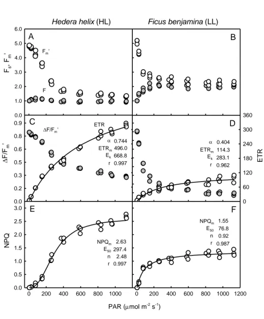
Light-response curves: ‘Single Pulse Light Curves’ 247
10 After defining AOIs matching the projected AALs (Fig. 4), the values of Fs and Fm’ were
248
determined for the various actinic light levels. These values were used to calculate indices 249
∆F/Fm’, rETR and NPQ that, when plotted against incident actinic light, resulted in
light-250
response curves (Fig. 5). These ‘Single Pulse Light Curves’ (SPLC),despite requiring just a few 251
minutes of light mask exposure and a single saturating pulse, nevertheless allowed to 252
characterize in detail the light response of the tested samples. Strong indications of the quality 253
of these light curves were the low variability between replicates (measurements on AALs of 254
identical PAR level, corresponding to a same row of the light mask), and the very good fit 255
obtained with well-establishedmathematical models for describing rETR and NPQ vsE curves. 256
The light-response patterns were consistent with the ones expected for LL- and HL-acclimation 257
states. Departing from similar Fv/Fm values, ∆F/Fm’ decreased more steeplywith increasing
258
irradiance in LL-acclimated F. benjamina than in HL-acclimated H. helix (Fig. 5B, E). This 259
resulted in distinct rETRvsE curves,with H. helix showing higher values for initial slope (α) 260
and, mainly, maximum rETR (rETRm, ca. 5 times higher than for F. benjamina). Also typical of
261
the difference between LL- and HL-acclimated samples, the photoacclimation indexEk was
262
much higher (more than double) in H. helixthan in F. benjamina, in accordance with the fact 263
that the former showed little signs of saturation even at 1125 µmol m-2 s-1, while the 264
lattersaturated at comparatively lowerPAR values (Fig. 5E).Also in the case of NPQ vsE curves, 265
the results were in agreement with expected LL- and HL-acclimation patterns, with H. helix 266
reaching higher maximum NPQ values (NPQm), requiring higher light levels for full
267
development (E50) and higher sigmoidicity (n).
268 269
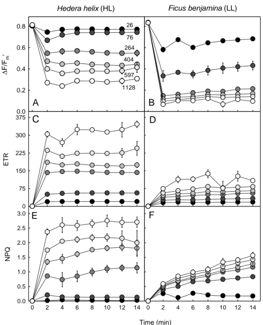
Dynamic light response 270
A further application of the method concerns the study of the temporal variation of the light 271
response. Figure 6 shows an example of the variation over time of ∆F/Fm’ rETR and NPQfor H.
272
helix and F. benjaminaduring lightinduction underdifferent PAR levels. Confirming the very 273
different light-response patterns observed before, this approach made it possible to additionally 274
compare the temporal variation of the response of each fluorescence index. For the HL-275
acclimated H. helix, ∆F/Fm’ and rETR stabilized quite rapidly, reaching a steady state within
4-276
6 min upon light exposure (Fig. 6A,C). The patterns of variation were essentially the same for 277
the different light levels, although stabilization was faster for the samples exposed to lower 278
PAR. For NPQ, steady state was reached only after 8-10 min, the induction pattern varying with 279
the light level applied (Fig. 6E).In the case of LL-acclimated F. benjamina, all indices took a 280
longer time to reach a steady state (Fig. 6 B,D,F). This was especially true for NPQ, which still 281
increased for most of the PAR levels after 14 min of light exposure. 282
This approach isalso particularly useful to follow the changes in the light-response curve 283
and to determine the time necessary for reaching of a steady-state. This can be achieved by 284
11 following the variation over time of the model parameters used to describe the light-response 285
curves. Using the dataset partially shown on Fig. 6, Fig. 7 shows the variation during light 286
induction of the parameters of rETR and NPQ vsEcurves. Regarding the rETRvsE curves, α was 287
the parameter that showed a smaller variation over time, increasing modestly until reaching 288
stable values after 6 and 10 min for H. helix and F. benjamina, respectively (Fig. 7A). In 289
contrast, rETRm and Ek showed much largerfluctuations, particularly for H. helix, requiring
290
more than 8-10 min for reaching relatively stable values (Fig. 7B, C).For the parameters of 291
NPQvsE curves, similar time periods of 6-10 min were necessary for reaching steady state 292
conditions (Fig. 7 D-F).However, despite the different induction patterns observed for HL-and 293
LL-acclimated samples, most of the differences observed at steady state were already present at 294
the first measurements(2-4 min). This indicates that even a short 2-4 min period of light mask 295
exposure may be sufficient to characterize LCs and detect differences between different light 296
acclimation states. 297
298
Light stress-recovery experiments and NPQ components 299
This approach can be easily extended to carry out light stress-recovery experiments, in which 300
samples are sequentially exposed to high light and then to darkness or low light, and the 301
fluorescence kinetics during light induction and dark relaxation is used to evaluate the operation 302
of photoprotective and photoinhibitory processes (Walters and Horton, 1991; Müller et al., 303
2001). Usually, only one light level is used, of arbitrarily chosen intensity(Rohácek, 2010; 304
Serôdio et al., 2012).By applying a light mask conveying a range of actinic light it becomes 305
possible to study the fluorescence kinetics during light induction and dark relaxation for 306
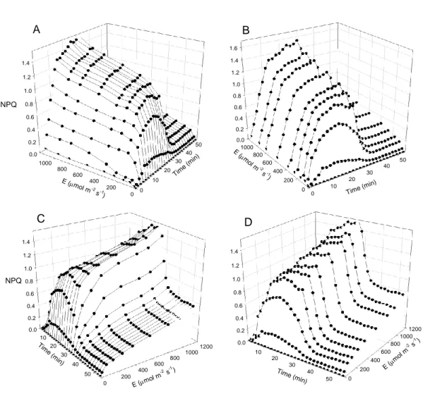
different PAR intensities simultaneously. 307
This is exemplified with the response of NPQ of LL-acclimated F. benjaminaduring light 308
induction and subsequent dark relaxation (Fig. 8).A large and detailed dataset was obtained 309
from a single leaf on the NPQ induction under various PAR levels (Fig. 8A, B) and on its 310
relaxation in the dark (Fig. 8C, D). Figure 8 also highlights the two types of information that 311
can be extracted from the same dataset: light-response curves (Fig. 8A,C) and 312
induction/relaxation kinetics (Fig. 8B,D). By applying the rationale used for the calculation of 313
NPQ components, such a dataset can be used to generate light-response curves of coefficients 314
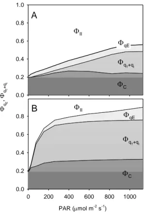
quantifying photoprotection capacity and susceptibility to photoinhibition(Guadagno et al., 315
2010). Figure 9 illustrates thisapproach by comparingthe repartition of absorbed light energy in 316
HL-acclimated H. helix and LL-acclimated F. benjamina. The former plant was shown to be 317
able to use a larger fraction of absorbed light for photochemistry (∆F/Fm’; ca. 0.5 above 800
318
µmol m-2 s-1; Fig. 9A) while non-photoprotective NPQ components (qT+qI) remained under 319
relatively low values (< 20%) and only started above 400 µmol m-2 s-1 (Fig. 9A).In contrast, for 320
the LL-acclimated F. benjamina ∆F/Fm’ was much lower throughout the light intensity range
12 (<0.2 for PAR as low as 400 µmol m-2 s-1; Fig. 9B) and NPQ started to increase under much 322
lower PAR levels, reaching maximum values at ca. 200 µmol m-2 s-1(qT+qI, qC). 323 324 325 DISCUSSION 326 327 Method assumptions 328
The purpose of this study was to demonstrate the proof of principle of the method, starting 329
by identifying and testing the conditions required for its general application. The successful 330
generation of non-sequential LCs using the combination of spatially separated actinic light 331
beams and imaging chlorophyll fluorescence implied the verification of two types of 332
assumptions:(i) assumptions associated to the projection of an actinic light mask and the 333
detection of the induced fluorescence response, and (ii) assumptions related to the use of a 334
digital projector as a source of actinic light for this purpose. These conditions were tested and 335
shown to be verified. 336
Regarding the projection of the actinic light mask, a very basic assumption of the method 337
was that the samples exposed to different actinic light levels must have essentially the same 338
inherent physiological light response, so that the fluorescence measured in different AALs may 339
be attributed to the different PAR irradiances applied. In a way, this approach is opposed to the 340
traditional use of chlorophyll fluorescence imaging systems: instead of applying a homogeneous 341
actinic light field to study heterogeneous samples, here aheterogeneous actinic light field is 342
applied to study supposedly homogeneous samples. The verification of this condition is mostly 343
dependent of the physiological heterogeneity on the samples. In some cases, as for suspensions 344
of microalgae or chloroplasts, samples can be prepared so that a uniform response can be 345
assured. However, in the case of leaves, it must be previously confirmed that the area to be used 346
for the measurements is homogeneous regarding its photophysiologicalresponses.The here 347
presented results showed that the method can be successfully applied to whole leaves, through 348
careful selection of uniform areas, in order to minimize the potentially confounding effects of 349
within-leaf spatial inhomogeneity. 350
Another key assumption of the method is the independence of the measurements. This 351
condition can be easily ensured by using optically separated samples, using cell or chloroplast 352
suspensions, or leaf disks in opaque multi well plates impeding the transmission of light 353
between adjacent samples. Potential problems are thus restricted to optically continuous 354
samplessuch as whole leaves, where light spillover from one AAL to another may result in a 355
lack of independence between adjacent AAL. This effect is analogue to the time dependency 356
between consecutive measurements during a sequential light curve. The results of the tests 357
performed on leaves showedthat this effect varied with species and with the leaf optical 358
13 properties affecting the amount of internal light scattering. However, they also showed that light 359
spillover can be greatly minimizedthrough adequate design of the actinic light mask (see 360
below). 361
Regarding the use of digital projectors as actinic light sources, two conditions appeared to 362
be of most importance: the maintenance of a constant spectrum throughout the range of applied 363
irradiances, and the elimination of effects of light flickering on fluorescence measurements. The 364
maintenance of a constant spectrum is important because changes of light spectrum can have 365
substantial effects on ∆F/Fm’, due to the variation of photosynthetic pigments absorptivity over
366
different wavelength ranges.This effect may be observed when comparing rETR light response 367
curves induced by monochromatic light of different colors (Schreiber et al., 2012). In the 368
present case, the enrichment of the green-yellow part of the spectrum is expected to cause and 369
overestimation of ∆F/Fm’, for the measured PAR, because light of these wavelengths are
370
comparatively less absorbed by the dominating pigments such as chlorophyll a and b, thus 371
inducing a smaller quenching of Fs and Fm’.Therefore, if the light spectrum varies between
372
different AALs, this will likely result in a deformation of the shape of the LC, resulting in an 373
artifactual absence of saturation or decline under high light.As shown here, this problem may be 374
tackled by digitally manipulating the spectrum of the emitted light. Despite some limitations, as 375
only the spectral ranges corresponding to the RGB coding can be manipulated, this approach 376
was shownto suffice to solve the effects of the changes in lamp output spectrum. Nevertheless, 377
the need for this corrective procedure will depend on the magnitude of the induced effects, in 378
turn dependent on the particular experimental and equipment conditionssuch as projector and 379
lamp type, and PAR levels to be used. 380
The elimination of effects of light flickering is important because light flickering was 381
shown to cause substantial interferences in the fluorescence record, particularly for high actinic 382
light levels, under which the difference between Fs and Fm’ is smaller and the error associated to
383
the determination of ∆F/Fm’ is higher. While affected fluorescence values may be easily
384
identified and eliminated from the calculation of Fs and Fm’, this requires the possibility to
385
access the raw fluorescence data, which may not be feasible with some PAM fluorometer 386
models or software. 387
388
Light mask design 389
A crucial piece of the proposed experimental approach is the actinic light mask used to 390
project spatially separated areas of actinic light. The light mask used in this study resulted from 391
a large number of preliminary tests on several aspects such as mask shape and dimension, as 392
well as number, size and disposition of the AALs. Its development followed some principles of 393
general applicability in designing light masks for similar studies: 394
14 i) Mask dimension. The shape and size of the light mask should consider thesample
395
dimensions as well as the homogeneity of the measuring light and saturating pulse light fields. 396
Smaller masks likely fit better within the zone of homogenous light field sampling area, while 397
they may also help to avoid heterogeneous parts of the sample (e.g. major leaf veins). On the 398
other hand, too small masks may limit both the total number and size of AALs, and, by 399
implying short distances between adjacent AALs, may increase light spillover and compromise 400
the independency of the measurements. 401
ii) Number of AALs. A large number of AALs allows for a large number of light levels, 402
which is useful for a good characterization of the light resposne, and for replication, reducing 403
variability and increasing precision of parameter estimation. However, the number of AALs 404
possible to accommodate will be limited by total mask size and by the spillover between 405
adjacent AALs. In the present study, it was possible to accommodate 30 AALs, which resulted 406
in a satisfactorily number of data points along the light curve and a good level of replication. By 407
effectively impeding light spillover (e.g. using opaque multi well plates), this number could be 408
significantly increased without increasing light mask size. 409
iii) AAL distribution pattern. In principle, AALs should be randomly distributed 410
throughout the light mask. This would minimize any systematic effects due to the AAL position 411
within the possibly inhomogeneous measuring light and saturating pulses fields. However, when 412
spillover effects cannot be completely avoided as in the case of whole leaves, better results were 413
found by arranging the AAL along a gradientof light intensity because in a randomized layout 414
there is a high chance of having adjacent AAL of very different light intensities, resulting in 415
substantial spillover and loss of measurement independency. When AALs are distributed along 416
a light intensity gradient, the light intensity of adjacent AALs will be more similar,thus reducing 417
the relative impact on each other.Besides preventing optical spillover, this design will also 418
minimize the potential exchange of light-induced metabolites between adjacent AALs, which 419
could contribute to some degree of non-independency between measurements, especially during 420
long light exposures, as for the study of dynamic light responses (see below). Although this 421
source of measurement dependencycannot be completely excluded for optically continuous 422
samples, its actual interference on the resulting light-response curve can be minimized by 423
decreasing the difference in light levels between AALs next to each other. 424
iv) AAL size. Large AALs should be used because more pixels will be considered for the 425
estimation of fluorescence parameters, therefore reducingmeasuring errors. This can be of value 426
in the case of samples showing a high physiological heterogeneity. Large AAL are also 427
preferable because the actual area used for calculation of fluorescence parameters (AOI) must 428
be smaller than the maximum diameter of AAL, to avoid the border effects. The light mask used 429
in this study had AALsof the same size and shape, disposed in linear arrays. However, masks 430
may have AAL of different size or shape and arranged in any other way, to better fit specific 431
15 aspects of the sample or sample container. For instance, because under higher actinic irradiances 432
a larger error is associated to the measurement of ∆F/Fm’,AAL of higher light levels could be
433
larger, resulting inmore precise measurements due to the higher pixel number. 434
435
Single Pulse Light Curves 436
The here proposed method for the generation of light-response curves presents a number of 437
innovations and significant advantages relatively to conventional approaches. It enables to: (i) 438
obtain non-sequential, temporally-independent fluorescence measurements; (ii) apply a large 439
and variable number of actinic light levels with adequate replication; (iii) generate a whole LC 440
within the time required for a single measurement; (iv) define and control with unprecedented 441
flexibility and ease of use the actinic light levels to be applied. 442
The considerable reduction of the total time required for the generation of a LC is one of 443
the major advantages of this approach. As all light levels and replicates are measured 444
simultaneously, the total duration of the LC will be essentially determined by the time defined 445
for each individual measurement (e.g. for reaching a steady-state), independently of the number 446
of light levels and replicates.For example, for the case shown in Fig. 5, the whole LC,consisting 447
of 30 measurements (10 light levels x 3 replicates),could be finished after 6 min of light 448
exposure, while it would have required a minimum of 3 hours if each light level/sample was 449
measured separately. This possibility is particularly useful when studying samples showing fast 450
changesin their physiological state, as a response to stressors or changing environmental 451
conditions, or associated to circadian rhythms (Rascher, 2001). 452
It is generally desirable for LCs to describe steady-state conditions. ‘Steady-state light 453
curves’ are largely independent from transient responses due to recent light history, making it 454
easier to characterize the inherent physiological light response of a sample and to compare 455
different samples. For the samples tested in this study, periods of 4-6 minutes of light mask 456
exposure were enough to ensure a good characterization of the light response, allowing the 457
estimating LC parameters and detecting differences in photoacclimation state. However, the 458
time necessary to reach steady-state conditions depends greatly on the sample physiological 459
state and previous light history. Also, because it is not likely that a steady state is reached at the 460
same time for all actinic light levels, it isnot possible to define a unique protocol for the 461
application of the SPLC. Its application to samples of unknown physiological response should 462
be preceded by the preliminary monitoring of the variation over time of the fluorescence 463
response under the different actinic light levels. 464
465
Dynamic light response 466
The proposed method also enables to incorporate time in the study of the light response. 467
The variation over time of fluorescence indices such as ∆F/Fm’, rETR or NPQ, like their light
16 induction and dark relaxation kinetics, is of obvious interest for the characterization of the 469
photophysiology of a sample. However, the patterns of variation during induction or relaxation 470
strongly depend on the level of actinic light applied. In this context, the possibility to follow the 471
response to various actinic light levels simultaneously saves time, making it considerably easier 472
to study the variation over time of the light response. This approach allowsto combine two types 473
of studies that are often carried out separately: (i) light-response curves, in which actinic light 474
intensity is varied while the time for measuring a response is arbitrarily fixed; (ii) 475
induction/relaxation kinetics, in which actinic light intensity is arbitrarily fixed and the response 476
is followed over time. It becomes thus possible to easily characterize the dynamic light response 477
of a sample, describing both how the response to light varies with time and how the response 478
kinetics varies with light. 479
An application of this possibilityis the construction of light-response curves of fluorescence 480
indices that require the comparison of measurements made at different times. This is the case of 481
the coefficients that quantify the partitioning of non-photochemical quenching in 482
photoprotective (rapidly reversible) and photoinhibitory (slowly reversible) components. In 483
most studies, these components are quantified for a single level of actinic light, usually 484
arbitrarily defined to represent a stressful condition. By applying the proposed method, it 485
became possible to easily generate light-response curves of the various quenching coefficients, a 486
task that requires following the NPQ relaxation kinetics after the exposure to various actinic 487
light levels, and that would otherwise be very time consuming. 488
489
Limitations 490
Despite the considerable advantages the here described method offers, there are a number 491
of potential limitations that must be considered. Although the results here presented are specific 492
to the particular projector model used, these general limitations are likely applicable to any 493
other models that share the same technology. 494
One limitation regards the range of actinic light levels possible to apply. On one hand, it 495
was not possible to obtain complete darkness, the minimum light intensity in the ‘dark’ AALs 496
being 5 µmol m-2 s-1. This was due both to the limitationsof the projector’s output contrast and 497
to the unavoidable light scattering originating from the illuminated areas. While this makes it 498
impossible to measure parameters that require dark adaptation, like Fo and Fm, with the
499
projector turned on, it does not affect significantly the construction of LCs, as 5 µmol m-2 s-1can 500
be considered sufficiently low for most applications. For the special case of NPQ vsE curves, 501
which require the measurement of Fm(in the dark), the best alternative is to cover the projector’s
502
lens, and determine Fm before the LC is started.
503
On the other hand, the maximum light intensity reached at the samples level may also 504
represent a limitation for the construction of LCs. In the case of the setup used in this study, the 505
17 maximum value of 1125 µmol m-2 s-1 can be considered low when compared to the values 506
reached by many commonly used PAM fluorometers, including imaging systems, generally 507
reaching values above 2000 µmol m-2 s-1. Nevertheless, the actual limitation caused by the 508
maximum light output will dependon the capacity to cover the relevant range of light intensities 509
for each particular sample. For the plants used in this study, the range of actinic irradiances 510
applied enabled to characterize with adequate detail the light response of the various 511
fluorescence parameters and indices, including the light-saturated part of the curve. 512
Another potential limitation derives from the relative low sensitivity of imaging 513
chlorophyll fluorometers. These imaging systems are based on CCD sensors which are less 514
sensitive than photodiodes or photomultipliers that equip the most common types of PAM 515
fluorometers. This limits the detection of fluorescence signals, especially under high actinic 516
light, when Fm’ is lower and more difficult to discriminate from the Fs level. Accordingly, some
517
manufacturers do not recommend measuring LCs with PAR levelsabove 700 µmol m-2 s-1 518
(Imaging-PAM, 2009). This low sensitivity is expected to be overcome by using samples with a 519
high chlorophyll a content, but may limit the use of dilute microalgae or chloroplast 520 suspensions. 521 522 Further applications 523
This study aimed to show the main and most immediate applications of the method. Its use 524
was illustrated on intact plant leaves, but it is potentially applicable to many other types of 525
photosynthetic samples, ranging from large plant leaves, lichens,flat corals, macroalgae or algal 526
biofilms (microphytobenthos, periphyton) to phytoplankton or suspensions of microalgae, 527
chloroplasts or thylakoid suspensions, the main limitation being the chlorophyll a concentration. 528
The use of optically separated samples, as in multi-well plates, is advantageous because it 529
eliminates light spillover effects and ensures the independence of the measurements. 530
The results shown here were obtained using light masks with AALs that only differed 531
regarding light intensity. However, the digital control of actinic light opens other possibilities. 532
One is to manipulate the duration of light exposure so that in the same experiment, replicated 533
samples are exposed to different light doses, given by different combinations of light intensity 534
and exposure duration. Also colormay in principle be digitally manipulated and light masks 535
made to incorporate AALs of different spectral composition. This would enable the possibility 536
to compare the spectral responses of fluorescence indices. 537
A major result of this study is the introduction of digitally controlled illumination as source 538
of actinic light for photophysiological studies involving PAM fluorometry. It provides 539
unprecedented flexibility in the control of the various aspects of projected actinic light field. As 540
this study showed, commercially-available models of digital projectors, used in combination 541
with commonly-available software, may provide a readily accessible and inexpensive way of 542
18 applying actinic light mask and generating SPLCs. However, such models were not built for this 543
purpose and their correct use requires some adaptations, namely regarding image flickering and 544
changes in light spectrum. We hope that this study may serve as guidelines for overcoming the 545
limitations of currently available projectors, and to stimulate the development of dedicated 546
equipment. 547
548 549
19 MATERIAL AND METHODS
550 551
Experimental Setup 552
The setup was comprisedof a combination of aPulse Amplitude Modulation (PAM) 553
imaging chlorophyll fluorometerand a digital projector, used as actinic lightsource (Fig.1). The 554
projector was positioned near the fluorometer’s CCD camera, in such a way that the projected 555
light incided on the center of the area monitored by the fluorometer’s camera (sampling area), 556
optimizing the detection of the induced chlorophyll fluorescence. The projector was also 557
positioned as vertically as possible (angle of 10º from vertical), to minimize asymmetries in the 558
projected light field, and as close as possible to the sample (ca. 40 cm from the projector lens to 559
the center of the sampling area), to maximize light intensity at the sample level. 560
561
Imaging chlorophyll fluorometer 562
The imaging chlorophyll fluorometer (Open FluorCAM 800-O/1010, Photon Systems 563
Instruments; Brno, Czech Republic) comprised four 13 x 13 cm LED panels emitting red light 564
(emission peak at 621 nm, 40 nm bandwidth) and a 2/3” CCD camera (CCD381) with an F1.2 565
(2.8-6 mm) objective.Two of the LED panels providedmodulated measuring light (< 0.1 µmol 566
m-2 s-1), and the other two provided saturating pulses (>7500 µmol m-2 s-1, 0.8 s). Chlorophyll 567
fluorescence images (512 x 512 pixels, 695-780 nm spectral range) were captured and processed 568
using the FluorCam7 software (Photon Systems Instruments; Brno, Czech Republic).When 569
measuring long sequences of fluorescence images (dynamic light response, see below), the 570
Fluorcam7 software was controlled by a AutoHotkey(version 1.1.09.00; available at 571
www.autohotkey.com) script written to automatically run the protocol used for applying 572
saturating pulses, save the fluorescence kinetics data for each measurement and export data as 573
text files for further processing. 574
575
Digital projector 576
All presented results were obtained using a LCD digital projector (EMP-1715, Epson, 577
Japan), comprising a mercury arc lampproviding a light output of 2700 lumens. Afocusing lens 578
was used to focus the projected images in the fluorometer’s sampling area. The projected light 579
field covered a rectangular area of ca. 14 x 10 cm.Projector settings were set to provide the 580
widest range of light intensities at the sample level. With the above described setup 581
configuration, PAR levels in the sampling area ranged between 5 and 1125µmol m-2 s-1.Actinic 582
PAR irradiance at the sample level was measured using a PAR microsensor (US-SQS/W, Walz; 583
Effeltrich, Germany), calibrated against a recently-calibrated flat PAR quantum sensor (MQ-584
200, Apogee Instruments; Logan, Utah, USA). 585
20 Actinic light mask
587
The digital projector was used to project anactinic light mask on the sampling area, 588
consisting of a set of spatially separated actinic light areas (AAL), covering the range of PAR 589
levels necessary to induce the fluorescence responses to be used to generate a light curve. The 590
actinic light mask used in this study consisted of 30 circular AALarranged in a 3 x 10 matrix, in 591
which each array of 10 AAL corresponded to 10 different PAR values (5-1125µmol m-2 s-1), 592
arranged increasingly so that the highest values were closer to the projector (Fig. 1). Each AAL 593
consisted of a circular homogeneous light field of 4 mm in diameter. Adjacent AALs of the 594
same array were separated by 1.0 mm. Three 10-AAL arrays were projected in parallel (1.5 mm 595
apart) so that approximately the same light levelswere applied on the three arrays. However, due 596
to some unavoidable degree of heterogeneity in the projected light field, a small variation (on 597
average < 2.5%) was presented among replicated AALs. 598
The light mask was designed in MS PowerPoint, using a code written in MS Visual Basic 599
to define the number, position, size and shape (slightly oval to compensate for the inclination of 600
the projector) of each AAL, as well as the light intensity and spectrum (through controlling the 601
RGB code, see below). This code was used to automatically control the PAR level of each 602
AAL, based on a relationship established between RGB settings and the PAR measured at the 603
sample level. 604
The chlorophyll fluorescence emitted at each AAL was measured by defining Areas of 605
Interest (AOI) using the FluorCam7 software. The AOIs were centered on the AALs but had a 606
smaller diameter (ca. 3 mm) to minimize border effects that could otherwise introduce 607
significant errors. On average each AOI consisted of 32pixels. 608
609
Actinic light spectrum 610
The spectrum of the light emitted by the digital projector was measured over a 350-1000 611
nm bandwidth with a spectral resolution of 0.38 nm, using a USB2000 spectrometer (USB2000-612
VIS-NIR, grating #3, Ocean Optics; Duiven, The Netherlands)(Serôdio et al., 2009). Light was 613
collected using a 400-µm diameter fiber optic (QP400-2-VIS/NIR-BX, OceanOptics)positioned 614
perpendicularly to a reference white panel (WS-1-SL Spectralon Reference Standard, Ocean 615
Optics) placed in the center of the sampling area of the fluorometer and the projected 616
lightfield.A spectrum measured in the dark was subtracted to all measured spectra to account for 617
the dark current noise of the spectrometer. Spectrawere smoothed using a 10-point moving 618 average filter. 619 620 Light-response curves 621
Light-response curves were generated by determining fluorescence parameters Fs and Fm’
622
for each AOI, each corresponding to a different irradiance level. Fs and Fm’ were measured by
21 averaging all pixel values of each AOI andaveraging the fluorescence intensity during the 2 s 624
immediately before the saturating pulse, and during 0.6 s during the application of the saturating 625
pulse (total duration of 800 ms), respectively.The kinetics of fluorescence intensity recorded 626
immediately before and during the application of each saturating pulsewas analyzed for each 627
measurement using the FluorCam7 software, and the parts of the fluorescence trace showing 628
effects of the projector’s light flickering were not considered for the estimation of Fs or Fm’. For
629
each AOI (each irradiance level, E), the relative rETR was calculated from the product of E and 630
the PSII effective quantum yield, ∆F/Fm' (Genty et al., 1990):
631 632 ' ' ' rETR m m s m F F E F F F E (1) 633 634
Fluorescence measurements were also used to calculate the non-photochemical quenching 635
(NPQ) index, used to quantify the operation of photoprotective and photoinhibitory processes. 636
NPQ was calculated from the relative difference between the maximum fluorescence measured 637
in the dark-adapted state, Fm, and upon exposure to light, Fm':
638 639 ' ' NPQ m m m F F F (2) 640 641
For each AOI, Fm was measured at the end of a 20 min dark adaptation prior to light
642
exposure. Light-response curves were generated by applying a single saturating pulse after a 643
defined period of light exposure (e.g. 6 min), following a 20 min dark-adaptation period. 644
645
Dynamic light response 646
The potentialities of the method were further tested by characterizing the dynamic light 647
response, i.e. the variation of the fluorescence light response over time. After a 20 min dark 648
adaptation, samples were exposed to the light mask and saturating pulses were applied every 2 649
min. This rationale was also applied to light stress-recovery experiments, during which samples 650
were subsequentlyexposed to darkness, to allow the characterization of the recovery after 651
exposure to the various actinic light intensities.Data was used to calculate light-response curves 652
and light kinetics (light induction and dark relaxation) of NPQ, as well as the quenching 653
coefficients partitioning NPQ into constitutive, photoprotective, photoinhibitory components, 654
following Guadagno et al. (2010). 655
656
Light-response curves models 657
22 rETRvsE curves were quantitatively described by fitting the model
658
ofEilers&Peeters(1988), and by estimating the parameters α (the initial slope of the curve), 659
rETRm (maximum rETR) and Ek (the light-saturation parameter):
660 661 c E b E a E E 2 ) rETR( (3) 662 where 663 664 c 1 α , ac b 1 rETR m and ac b c E k (4) 665 666
Light-response curves of NPQ were described by fitting the model of Serôdio & Lavaud (2011), 667
and by estimating the parameters NPQm (maximum NPQ), E50 (irradiance corresponding to half
668
of NPQm) and n (sigmoidicity parameter):
669 670 n n n m E E E E 50 NPQ ) ( NPQ (5) 671 672
The models were fitted using a procedure written in MS Visual Basic and based on MS Excel 673
Solver. Model parameters were estimated iteratively by minimizing a least-squares function, 674
forward differencing, and the default quasi-Newton search method(Serôdio and Lavaud, 2011). 675
676
Plant material 677
The applicability of the method was illustrated on intact plant leaves. To compare the 678
method in samples having distinct light responses, plants acclimated to contrasting light 679
conditions were used.For high-light acclimated plants, leaves of Hedera helix L. (common ivy) 680
grown under natural conditions were used. Photoperiod and weather conditions were those of 681
November-December 2012 in Aveiro, Portugal: 10/14 h photoperiod, temperature range of 4-16 682
ºC, relative humidity of 60-80%, precipitation of 100-200 mm, 95-120 insolation hours. For 683
low-light acclimated plants, leaves of Ficusbenjamina L. (weeping fig) grown in a greenhouse 684
during the same time of year were used (average PAR of 20 µmol m-2 s-1).All plants were grown 685
in standard horticultural soil, and watered every two days. These two species were selected also 686
to illustrate the variability among leaf optical properties potentially affecting the measuring of 687
fluorescence in closely located illuminated areas (light scattering within the leaf). Unless stated 688
otherwise, all fluorescence measurements were made in the upper (adaxial) surface of the 689
leaves. 690
23 List of abbreviations
691 692
α - Initial slope of the rETR vs. E curve 693
a, b, c – parameters of the Eilers and Peeters (1988) model 694
AAL – Areas of Actinic Light 695
AOI – Areas of interest 696
∆F/Fm’ – Effective quantum yield of PSII
697
E– PAR irradiance (µmol photons m-2 s-1) 698
E50 – Irradiance level corresponding to 50% of NPQm in a NPQ vs. E curve
699
Ek– Light-saturation parameter of the rETR vs. E curve
700
rETR – PSII relative electron transport rate 701
rETRm – MaximumrETR in a rETR vs. E curve
702
Fo, Fm – Minimum and maximum fluorescence of a dark-adapted sample
703
Fs, Fm’ – Steady state and maximum fluorescence of a light-adapted sample
704
Fv/Fm – Maximum quantum yield of PSII
705 HL – High light 706 LC – Light-response curve 707 LL – Low light 708
n – Sigmoidicity coefficient of the NPQ vs. E curve 709
NPQ – Non-photochemical quenching index 710
NPQm – Maximum NPQ value reached in a NPQ vs. E curve
711
PSII – Photosystem II 712
ΦqC– quantum yield of chlorophyll photophysical decay
713
ΦqE–quantum yield of energy-dependent quenching
714
ΦqT+qI – quantum yield of state transition and photoinhibitory quenching
715
SPLC – Single Pulse Light Curve 716
24 ACKNOWLEDGEMENTS
718
We thank Gonçalo Simões for invaluable technical help on testing of digital projectors. This 719
work benefited from discussions with Sónia Cruz, Jorge Marques da Silva, Paulo Cartaxana, 720
and David Suggett. 721
25 REFERENCES
723 724
Eilers PHC, Peeters JCH (1988) A model for the relationship between light intensity and the 725
rate of photosynthesis in phytoplankton. Ecol Model 42: 199–215 726
727
Genty B, Briantais JM, Baker NR (1989)The relationship between the quantum yield of 728
photosynthetic electron transport and quenching of chlorophyll fluorescence. 729
BiochimBiophysActa990: 87–92 730
731
Genty B, Harbinson J, Baker NR (1990)Relative quantum efficiencies of the two 732
photosystems of leaves in photorespiratory and non-photorespiratory conditions. Plant 733
PhysiolBiochem28: 1–10 734
735
Guadagno CR, Virzo De Santo a, D’Ambrosio N (2010) A revised energy partitioning 736
approach to assess the yields of non-photochemical quenching 737
components.BiochimBiophysActa1797: 525–530 738
739
Henley WJ (1993)Measurement and interpretation of photosynthetic light-response curves in 740
algae in the context of photoinhibition and diel changes. J Phycol29: 729–739 741
742
Herlory O, Richard P, Blanchard GF (2007) Methodology of light response curves: 743
application of chlorophyll fluorescence to microphytobenthic biofilms. Mar Biol153: 91–101 744
745
Ihnken S, Eggert A, Beardall J (2010) Exposure times in rapid light curves affect 746
photosynthetic parameters in algae. Aquat Bot 93: 185–194 747
748
Imaging-PAM, M-Series Chlorophyll fluorometer, Instrument description and information for 749
users (2009). Heinz Walz GmbH, Effeltrich 750
751
Johnson ZI, Sheldon TL (2007)A high-throughput method to measure photosynthesis-752
irradiance curves of phytoplankton. LimnolOceanogr Meth 5: 417–424 753
754
Lavaud J, Strzepek RF, Kroth PG (2007)Photoprotection capacity differs among diatoms: 755
Possible consequences on the spatial distribution of diatoms related to fluctuations in the 756
underwater light climate. LimnolOceanogr52: 1188–1194 757
26 Lefebvre S, Mouget J-L, Lavaud J (2011) Duration of rapid light curves for determining the 759
photosynthetic activity of microphytobenthos biofilm in situ. Aquat Bot95: 1–8 760
761
Müller P, Li XP, Niyogi KK (2001)Non-photochemical quenching.A response to excess light 762
energy. Plant Physiol125: 1558–1566 763
764
Perkins RG, Mouget JL, Lefebvre S, Lavaud J (2006)Light response curve methodology and 765
possible implications in the application of chlorophyll fluorescence to benthic diatoms. Mar 766
Biol149: 703–712 767
768
Ralph PJ, Gademann R (2005)Rapid light curves: a powerful tool to assess photosynthetic 769
activity. Aquat Bot 82: 222–237 770
771
Rascher U (2001)Spatiotemporal variation of metabolism in a plant circadian rhythm: The 772
biological clock as an assembly of coupled individual oscillators. ProcNatlAcadSci USA 98: 773
11801–11805 774
775
Rascher U, Liebig M, Lüttge U (2000)Evaluation of instant light-response curves of 776
chlorophyll fluorescence parameters obtained with a portable chlorophyll fluorometer on site in 777
the field. Plant Cell Environ 23: 1397–1405 778
779
Rohácek K (2010)Method for resolution and quantification of components of the non-780
photochemical quenching (qN). Photosynth Res 105: 101–113
781 782
Schreiber U, Bilger W, Neubauer(1994)Chlorophyll fluorescence as a nonintrusive indicator 783
for rapid assessment of in vivo photosynthesis.In: ED Shulze, MM Caldwell, eds,Ecophysiology 784
of Photosynthesis. Springer-Verlag, Berlin,pp 49– 70 785
786
Schreiber U, Schliwa U, Bilger W (1986) Continuous recordingof photochemical and 787
nonphotochemical chlorophyll fluorescencequenching with a new type of modulation 788
fluorometer. Photosynth Res 10: 51–62 789
790
Schreiber U, Gademann R, Ralph PJ, Larkum AWD (1997)Assessment of photosynthetic 791
performance of Prochloron in Lissoclinum patella in hospite by chlorophyll fluorescence 792
measurements. Plant Cell Physiol38: 945–951 793
27 Schreiber U, Klughammer C, Kolbowski J (2012)Assessment of wavelength-dependent 795
parameters of photosynthetic electron transport with a new type of multi-color PAM chlorophyll 796
fluorometer. Photosynth Res 113: 127–144 797
798
Seaton GGR, Walker DA (1990)Chlorophyll fluorescence as a measure of photosynthetic 799
carbon assimilation. Proc Royal SocLond B 242: 29–35 800
801
Serôdio J, Cartaxana P, Coelho H, Vieira S (2009) Effects of chlorophyll fluorescence on the 802
estimation of microphytobenthos biomass using spectral reflectance indices. Rem Sens Environ 803
113: 1760–1768 804
805
Serôdio J, Ezequiel J, Barnett A, Mouget J, Méléder V, Laviale M, Lavaud J (2012) 806
Efficiency of photoprotection in microphytobenthos: role of vertical migration and the 807
xanthophyll cycle against photoinhibition. AquatMicrobEcol67: 161–175 808
809
Serôdio J, Lavaud J (2011) A model for describing the light response of the nonphotochemical 810
quenching of chlorophyll fluorescence. Photosynth Res 108: 61–76 811
812
Serôdio J, Vieira S, Cruz S, Barroso F (2005) Short-term variability in the photosynthetic 813
activity of microphytobenthos as detected by measuring rapid light curves using variable 814
fluorescence. Mar Biol146: 903–914 815
816
Serôdio J, Vieira S, Cruz S, Coelho H (2006) Rapid light-response curves of chlorophyll 817
fluorescence in microalgae: relationship to steady-state light curves and non-photochemical 818
quenching in benthic diatom-dominated assemblages. Photosynth Res 90: 29–43 819
820
Smith EL (1936) Photosynthesis in relation to light and carbon dioxide. ProcNatlAcadSci USA 821
22: 504–511 822
823
Walters RG, Horton P (1991) Resolution of components of non-photochemical chlorophyll 824
fluorescence quenching in barley leaves. Photosynth Res 27: 121–133 825
826
White AJ, Critchley C (1999) Rapid light curves: a new fluorescence method to assess the 827
state of the photosynthetic apparatus. Photosynth Res 59: 63–72 828
28 Ye Z-P, Robakowski P, Suggett DJ (2012) A mechanistic model for the light response of 830
photosynthetic electron transport rate based on light harvesting properties of photosynthetic 831
pigment molecules. Planta237: 837-847 832