Reactive Programming of Simulations in Physics

HAL Id: hal-01074901

https://hal-mines-paristech.archives-ouvertes.fr/hal-01074901

Preprint submitted on 15 Oct 2014

HAL is a multi-disciplinary open access

archive for the deposit and dissemination of

sci-entific research documents, whether they are

pub-lished or not. The documents may come from

L’archive ouverte pluridisciplinaire HAL, est

destinée au dépôt et à la diffusion de documents

scientifiques de niveau recherche, publiés ou non,

émanant des établissements d’enseignement et de

Reactive Programming of Simulations in Physics

Frédéric Boussinot, Bernard Monasse, Jean-Ferdy Susini

To cite this version:

Frédéric Boussinot, Bernard Monasse, Jean-Ferdy Susini. Reactive Programming of Simulations in

Physics. 2014. �hal-01074901�

Reactive Programming

of Simulations in Physics

Frédéric Boussinot

Mines-ParisTech, Cemef

Bernard Monasse

Mines-ParisTech, Cemef

Jean-Ferdy Susini

CNAM, Cédric

October 15, 2014

We consider the Reactive Programming (RP) approach to simulate physical systems. The choice of RP is motivated by the fact that RP genuinely offers logical parallelism, instantaneously broadcast events, and dynamic creation/destruction of parallel components and events. To il-lustrate our approach, we consider the implementation of a system of Molecular Dynamics, in the context of Java with the Java3D library for 3D visualisation.

Keywords. Concurrency ; parallelism ; reactive programming ; physics ; molecular dynamics.

1

Introduction

The essence of programming is to manipulate data structures through proce-dures [12]. Objects which group (encapsulate) data and the procedures (meth-ods) to use them is at the basis of object-oriented programming. When the decomposition into objects is adequate, object programming is usually consid-ered as leading to more natural and safer programs as it reduces the distance between the programmer’s intuition and the program structure. For example, let us consider a physical system made of atoms. In an object-oriented approach, an atom is quite naturally represented by an object containing the atom state (e.g. position, velocity, and mass) and the procedures to transform the atom state (e.g. computing the next position).

Some systems to simulate physics are coded with objects as LAMMPS, pro-grammed in C++ [13]. As more traditional systems programmed in Fortran

(e.g. DL_POLY [14]), their central structure basically consists in arrays stor-ing data, and loops to process the array elements in turn. A general issue with such structures is the difficulty to add (and to remove) data, or objects, during the course of a simulation (dynamically). Some molecular simulation systems are able to deal with dynamic creation of chimical bonds (this is for exam-ple the case of LAMMPS, in which the ReaxFF [5] potential is implemented), but, to our knowledge, no simulation system is able to deal with the dynamic creation/destruction of general components (e.g. atoms).

The dynamic creation/destruction of components can be useful to model multi-scale systems [4], in which the scale of sub-systems is allowed to change during execution. Let us consider, a molecule simulated at the All-Atom (AA) scale; when the molecule is isolated from the others, il may be possible to switch its scale to Coarse-Grained (CG) and thus to simulate the molecule more efficiently. The inverse scale change may be mandatory when molecules become so close that their interactions must be described at the lowest AA level. In both cases, a change of scale can be seen as the replacement of the molecule by a new one. For example, the AA to CG change of scale consists in the creation of a new CG molecule, simultaneous with the destruction of the old AA molecule.

In this text, we propose an approach to the implementation of physical simulations in which the dynamic creation or destruction of components can be simply and naturally expressed. The objective is the design of a Molecular Dynamics (MD) system allowing multi-scale modeling. We use a programming approach, called Reactive Programming (RP) [2], with a generalized notion of object: an object encapsulates not only its data and methods to manipulate them, but also its behaviour which can be used to code its interactions with the other objects. In this context, a simulation is structured as an assembly of interacting objects whose behaviours are run in a coordinated way, by an execution machine able to dynamically create and run new objects, and to destroy others.

Structure of the Paper

The paper is structured as follows: Section 2 justifies the use of RP for the implementation of physical simulations. Section3 describes RP in general and more precisely the SugarCubes framework. MD is described in Section4. The implementation of the MD simulation system is described in Section5. Related work is considered in Section6, and Section7concludes the paper, giving several tracks for future work.

2

Rationale

When it is not possible, while considering a physical system, to find exact an-alytical solutions describing its dynamics, the numerical simulation approach becomes mandatory. Numerical simulations are based, first, on a discretization of time and second, on a stepwise resolution method implementing an

integra-tion algorithm. The possibility to get analytical soluintegra-tions is basically limited by complexity issues: complex systems cannot usually be analytically solved. This renders numerical simulations an important topics for physics.

Parallelism. At the logical level, it is often the case that the processing of a complex system is facilitated by decomposing it into several sub-systems linked together. The sub-systems can thus be considered as independent components, running and interacting in a coordinated way. Recast in the terminology of informatics, one would say that the sub-systems are run in parallel in an envi-ronment where they share the same notion of time. Here, we are not speaking of real time but of a logical time, shared by all the sub-systems. In this approach, the steps of the numerical resolution method used to simulate the system have to be mapped onto the logical time; we shall return on this subject later. Since we are assuming time to be logical, we should also qualify parallelism as being logical: parallelism is not introduced here to accelerate execution (for example, by using several processors) but to describe a complex system as a set of paral-lel entities. The use of real-paralparal-lelism (offered by multiprocessor and multicore machines) to accelerate simulations is of course a major issue, but we think that it is basically a matter of optimisation, while the use of logical parallelism is basically a matter of expressivity.

Determinism. Simulations of physical systems must verify a strong and man-datory constraint: no energy should be either created or destroyed during the simulation of a closed system (without interaction with the external world). In other words, total energy1_{must be preserved during the simulation process. This}

is a fundamental constraint: it corresponds to the reversibility in time of the Newton’s laws which is at the basis of classical physics. This constraint can be formulated differently: classical physics is deterministic. In informatics, this has a deep consequence: as physical simulations should be deterministic, one should give the preference to programming languages in which programs are deterministic by construction. Note however, that parallelism and determinism do not usually go well together; there are very few programming languages which are able to provide both; we shall return on this point later.

Broadcast events. In addition to time reversibility, classical physics rests on a second fundamental assumption: forces (gravitation, electrostatic and inter-atomic forces) are instantaneously transmitted2_{. Instantaneity in our case}

should accommodate with the presence of the logical time; actually, instanta-neity means that action/reaction forces (third Newton’s law) should always be exerted during the same instant of the logical time. It is in the nature of classical physical forces to be broadcast everywhere. In informatics terms, forces corre-spond to information units that are instantaneously broadcast to all parallel components. This vision of forces actually identifies forces with instantaneously

1

Total energy is the sum of potential energy and kinetic energy.

2

broadcast events; we shall see that this notion of instantaneously broadcast event exists in the so-called synchronous reactive formalisms, which thus appear to be good candidates to implement physical simulations.

Modularity. It may be the case that some components of a system have to be removed from the system because their simulation is no more relevant (imagine for example an object whose distance from the others becomes greater than some fixed threshold, so that its contribution may be considered as negligible). Destruction of components is usually not a big issue in simulations: in order to remove an object from the global system, it may be for example sufficient to stop considering it during the resolution phase. Dually, in some situation, new components may have to be created, for example in chemistry where chemical bonds linking two atoms can appear in the course of a simulation. Dynamic creation is more difficult to deal with than destruction; for example, a new created object must be introduced only at specific steps of the resolution method, in order to avoid inconsistencies. In informatics terms, both dynamic destruction and dynamic creation of parallel components should be possible during the course of simulations. This possibility is often called modularity: in a modular system, new components can appear or disappear during execution, without need to change the other components. Note that the notion of broadcast event fits well with modularity as the introduction of a new component listening or producing an event, or the removal of an already existing one, does not affect the communication with the other parallel components.

Hybrid systems. There exist hybrid physical systems which mix continuous and discrete aspects. For example, consider a ball linked by a string to a fixed pivot and turning around the pivot (continuous aspect); one can then consider the possibility for the string to be broken (discrete aspect). Numerical simula-tions of hybrid systems are more complex than those of standard systems: in the previous example, the string component has to be removed from the simu-lation when the destruction of the string occurs, and the simusimu-lation of the ball has to switch from a circle to a straight line. In this respect, a hybrid system can be seen as gathering several related systems (for example, the system where the ball is linked to the pivot, and the system where it is free) ; then, the issue becomes to define when and how to switch from one system to another. Note that the simulation of hybrid systems is related to modularity: in the previ-ous example, one can consider that the breaking of the string entails on the one hand the destruction of both the string component and the circular-moving ball, and on the other hand the simultaneous creation of a straight-moving new ball appearing at the position of the old one.

Resolution method. Let us discuss now the relation between logical time and the discretized time of the resolution method. We shall call instant the basic unit of the logical time; thus, a simulation goes through a first instant,

then a second, and so on, until termination3_{. The only required property of}

instants is convergence: all the parallel components terminate at each instant. Execution of instants does not necessarily take the same amount of real time; actually, real time becomes irrelevant for the logic of simulations: the basic simulation time is the logical time, not the real time. The numerical resolution method works on a time discretized in time-steps during which forces integration is performed according to Newton’s second law. Typically, in simulations of atoms, time-steps have a duration of the order of the femto-second. Several steps of execution may be needed by the resolution algorithm to perform one time-step integration; for example, two steps are needed by the velocity-Verlet integration scheme [18] to integrate forces during one time-step: positions are computed during the first step, and velocities during the second. Actually, a quite natural scheme associates two instants with each time-step: during the first instant, each component provides its own information; the global information produced during the first instant is then processed by each component during the second instant. Note that such a two-instant scheme maps quite naturally to the velocity-Verlet method: each step of the resolution method is performed during one instant.

Multi-time aspects. The use of the same time-step during the whole simu-lation is not mandatory : one calls multi-time a system in which the time-step of the resolution method is allowed to vary during the simulation.

The change of time-step can be global, meaning that it concerns all the objects present in the simulation. This can be helpful for example to get a more accurate simulation when a certain configuration of objects is reached (for example, when objects become confined in a certain volume).

Alternatively, the change of time-step can be local, i.e. concerning only cer-tain objects, but not all. This means that different components of the same simulation are simultaneously simulated using different time-steps. This could be the case for a system in which diffusion aspects occur; in such a system, objects in some regions are separated by large distances and evolve freely, simu-lated with large time-steps, while in other regions, objects are closely interacting and should thus be simulated using smaller time-steps. We will return later on a situation of this kind. We shall call such systems multi-time, multi-step systems (MTMS systems, for short). A major interest of MTMS is that loosely-coupled objects (with rare interactions) can be simulated during long time periods.

In this text, we consider the Reactive Programming [2] (RP) approach to simulate physical systems. The choice of RP is motivated by the fact that RP genuinely offers logical parallelism, instantaneously broadcast events, and dy-namic creation/destruction of parallel components and events. Moreover, we choose a totally deterministic instance of RP, called SugarCubes [10], based on the Java programming language: indeed, in SugarCubes, programs are de-terministic by construction. To illustrate our approach, we shall consider the

3

implementation of a MTMS simulation system of Molecular Dynamics [6] (MD) in the context of Java, with the Java3D library [1] for 3D visualisation.

3

Reactive programming

Reactive Programming [2] (RP) offers a simple framework, with a clear and sound semantics, for expressing logical parallelism. In the RP approach, systems are made of parallel components that share the same instants. Instants thus define a logical clock, shared by all components. Parallel components synchronise at each end of instant, and thus execute at the same pace. During instants, components can communicate using instantaneously broadcast events, which are seen in the same way by all components. There exists several variants of RP, which extend general purpose programming languages (for example, ReactiveC [7] which extends C, and ReactiveML [15] which extends the ML language). Among these reactive frameworks is SugarCubes [10], which extends Java. In SugarCubes, the parallel operator is very specific: it is totally deterministic, which means that, at each instant, a SugarCubes program has a unique output for each possible input. Actually, in SugarCubes parallelism is implemented in a sequential way.

Due to its “determinism by construction”, we have choosen to use the Sug-arCubes framework to implement the MD system; we are going to describe SugarCubes in the rest of the section4_.

SugarCubes

The two main SugarCubes classes are Instruction and Machine. Instruction is the class of reactive instructions which are defined with reference to instants, and Machine is the class of reactive machines which run reactive instructions and define their execution environment.

The main instructions of SugarCubes are the following (their names always start by the prefix SC):

Void statement: SC.nothingdoes nothing and immediately terminates.

Next instant: SC.stopdoes nothing and suspends the execution of the running thread for the current instant; execution will terminate at the next instant. Sequence: SC.seq (inst1,inst2)behaves like inst1 and switches immediately to

inst2as soon as inst1 terminates.

Parallelism: SC.merge (inst1,inst2)executes one instant of instructions inst1 and inst2 and terminates if both inst1 and inst2 terminate. Execution al-ways starts by inst1 and switches to inst2 when inst1 either terminates or suspends.

4

We only describe the notions that are needed for the paper to be self-contained; a complete description of SugarCubes can be found in [10].

Cyclic execution: SC.loop (inst) executes cyclically inst: execution of inst is imme-diately restarted as soon as it terminates. One supposes that it is not possible for inst to terminate at the same instant it is started (otherwise, one would get an instantaneous loop which would cycle forever during the same instant, preventing thus the reactive machine to detect the end of the current instant).

Java code: SC.action (jact)runs the execute method of the Java action jact (of type JavaAction) (this can happen several time, as the action can be in a loop).

Event generation: SC.generate (event,value)generates event, with value as associated value, and immediately terminates.

Event waiting: SC.await (event)terminates immediately if event is present (i.e. it has been previously generated during the current instant), otherwise, execu-tion is suspended waiting either for the generaexecu-tion of event or for the end of the current instant, detected by the reactive machine.

Event values: SC.callback (event,jcall) executes the Java callback jcall (of type JavaCallback) for each value generated with event during the current instant. In order not to lose possibly generated values, the execution of the instruction lasts during the whole instant and terminates at the next instant.

Preemption: SC.until (event,inst) executes inst and terminates either because instterminates, or because event is present.

The sequence and merge operators are naturally extended to more than two branches; for example SC.seq (i1,i2,i3) is the sequence of the three instruc-tions i1,i2,i3.

A reactive machine of the class Machine runs a program (of type Program) which is an instruction (initially SC.nothing). New instructions added to the machine are put in parallel (merge) with the previous program. Addings of new instructions do not occur during the course of an instant, but only at beginnings of instants.

Basically, a machine cyclically runs its program, detects the end of the cur-rent instant, that is when all branches of merge instructions are all terminated or suspended, and then goes to the next instant.

Note that the execution of an instruction by a machine during one instant can take several phases: for example, consider the following code, supposing that event e is not already generated:

1 SC . merge ( SC . a w a i t e , 3 SC . g e n e r a t e ( e , n u l l ) )

Execution switches to the await instruction (line 2) which is suspended, as e is not present. Then, execution switches to the generate instruction (line 3),

which produces e and terminates. The executing machine detects that execution has to be continued, because one branch of a merge instruction is suspended, awaiting an event which is present. Thus, the await instruction is re-executed, and it now terminates, as e is present. The merge instruction is also now terminated.

The execution of a program by a machine is totally deterministic: only one trace of execution is possible for a given program. The execution of SugarCubes programs is actually purely sequential: the parallelism presently offered by Sug-arCubes is a logical one, not a real one; the issue of real parallelism is considered in Sec. 7.

4

Molecular Dynamics

Numerical simulation at atomic scale predicts system states and properties from a limited number of physical principles, using a numerical resolution method implemented with computers. In Molecular Dynamics (MD) [6] systems are organic molecules, metallic atoms, or ions. The goal is to determine the temporal evolution of the geometry and energy of atoms.

At the basis of MD is the classical (newtonian) physics, with the fundamental equation:

− →

F = m−→a

where−→F is the force applied to a particle of mass m and−→a is its acceleration (second derivative of the variation of the position, according to time).

A force-field is composed of several components, called potentials (of bonds, valence angles, dihedral angles, van der Waals contributions, electrostatic contri-butions, etc.) and is defined by the analytical form of each of these components, and by the parameters caracterizing them. The basic components used to model molecules are the following:

• _{atoms, with 6 degrees of freedom (position and velocity);}

• _{bonds, which link two atoms belonging to the same molecule; a bond} between two atoms a, b tends to maintain constant the distance ab. • _{valence angles, which are the angle formed by two adjacent bonds ba et bc}

in a same molecule; a valence angle tends to maintain constant the angle c

abc. A valence angle is thus concerned by the positions of three atoms. • _{torsion angles (also called dihedral angles) are defined by four atoms a, b, c, d}

consecutively linked in the same molecule: a is linked to b, b to c, and c to d; a torsion angle tends to priviledge particular angles between the planes abc and bcd.

• _{van der Waals interactions apply between two atoms which either belong} to two different molecules, or are not linked by a chain of less than three

(or sometimes, four) bonds, if they belong to the same molecule. They are pair potentials.

All these potentials depend on the nature of the concerned atoms and are parametrized differently in specific force-fields. Molecular models can also con-sider electrostatic interactions (Coulomb’s law) which are pair potentials, as van der Waals potentials are; their implementation is close to van der Waals potentials, with a different dependence to distance.

Intra-molecular forces (bonds, valence angles, torsion angles) as well as inter-molecular forces (van der Waals) are conservative: the work between two points does not depend on the path followed by the force between these two points. Thus, forces can be defined as derivatives of scalar fields. From now on, we consider that potentials are scalar fields and we have:

− →

F (r) = −−→∇ U_(r)

where r denotes the coordinates of the point on which the force−→F (r) applies, and U is the potential from which the force derives.

The precise definition of the application of forces according to a specific force-field (namely, the OPLS force-field [11]) is described in detail in [16], from which we have taken the overall presentation of MD.

We now describe the rationals for the choice of RP to implement MD.

Reactive programming for molecular dynamics

The choice of RP, and more specifically of SugarCubes, is motivated by the following reasons:

• _{MD systems are composed of separate, interacting components (atoms} and molecules). It seems natural to consider that these components ex-ecute in parallel. In standard approaches, there is generally a “big loop” which considers components in turn (components are placed in an array). This structuration is rather artificial and does not easily support dynamic changes of the system (for example, additions of new components or re-movals of old ones, things that one can find in modeling chemical reac-tions).

• _{In MD simulations, time is discrete, and the resolution method which is} at the heart of simulations is based on this discrete time. In RP, time is basically discrete, as it is decomposed in instants. Thus, RP makes the discretisation of time which is at the basis of MD very simple.

• _{MD is based on classical (Newtonian) physics which is deterministic. The} strict determinism of the parallel operator provided by SugarCubes reflects the fundamental determinism of Newtonian physics. At implementation level, it simplifies debugging (a faulty situation can be simply reproduced). At the physical level, it is mandatory to make simulations reversible in time.

• _{In classical physics, interactions are instantaneous which can be quite} naturaly expressed using the instantaneously broadcast event notion of RP.

In conclusion, the use of RP for MD simulations is motivated by its following characteristics: modularity of logical parallelism, intrinsic discretisation of time due to instants, strict determinism of the parallel operator, instantaneity of events used to code interactions.

Let us now consider the use of RP to implement Molecular Dynamics.

5

MD system

A molecular system consists in a set of molecules, each molecule being made of atoms, bonds, valence angles and torsion angles. In the approach we propose, the molecule components (atoms, bond, angles) are programs that are executed under the supervision of another main program called a reactive machine. The reactive machine is in charge of executing the components in a coordinated way, allowing them to communicate through events. Events are broadcast to all the components run by the reactive machine, that is, all components always “see” an event in the same way: either it is present for all components if it is generated by one of them, or it is absent for all components if it is not generated during the instant. All events are reset to absent by the reactive machine at the beginning of each instant. Values can be associated with event generations. In order to process the values generated with an event, a component has to wait during the whole instant, processing the values in turn, as they are generated.

The reactive machine proceeds in instants: the first instant is executed, then the second, and so on indefinitely. All components (atoms, bonds, etc) in the machine are run at each instant and there is an implicit synchronization (synchronization barrier) of all the components at the end of each instant. In this way, one is sure that all component have finished their reaction for the current instant and have processed all the generated events and all their values before the next instant can start. Basically, this mode of execution is synchronous parallelism.

The steps of the resolution method (velocity-Verlet) are identified with the instants of the reactive machine. The positions of atoms are computed during one step of the resolution method, and the velocities during the next step. Actually, at each instant, atoms generate their position and collect the various forces exerted on them (by bonds, angles, etc). The new positions are computed from previously collected information at even5 _{instants and the new velocities}

are computed at odd instants, following the two-step scheme of the velocity-Verlet numerical resolution method.

Note that the new positions and velocities are computed by the atom itself: we say that they are parts of the atom behavior. Strictly speaking, an atom

5

The choice of even or odd instants is arbitrary; the only requirement is actually that instants come in pairs.

is a structure that encapsulates data (in particular, position and velocity) to-gether with a behavior which is a program intended to be run by the reactive machine in which the atom is added. The good programming practice is that the atom’s behavior is the only component that should access the atom’s data. This discipline entails the absence of time-dependent errors. As direct access to the atom’s data is unwilled, events are the only means for a component to influ-ence an atom. For example, in order to apply a force to an atom, a component generates an event whose value is the force; the atom should wait for the event and process the generated values; in this way, the atom is able to process the force applied to it.

The constuction of molecules is a program whose execution adds the molecule components into the reactive machine. The main steps to simulate a molecular system are: 1) define a reactive machine; 2) run a set of molecules in order to add them in the machine; 3) cyclically run the machine.

In the rest of this section, we give a brief overview of the various programs that are used to build a simulation. Note that these are small pieces of code, that we hope to be natural and easily readable. This depart from standard MD system descriptions, which are usually decomposed in procedures whose chaining of calls is poorly specified. In our approach, the scheduling of the various sub-programs is made clear and unambiguous.

We shall first describes (generic and specific) atoms, then intra-molecular components (bonds and angles). We will also consider inter-molecular interac-tions. Then, we will explain how molecules are built from the previous atoms and components.

5.1

Atoms

An atom cyclically collects the constraints issues from bonds, valence angles, and dihedrals, then computes one step of the resolution method, and finally visualizes itself. This behavior can be preempted by a kill signal (generated for example when the molecule to which the atom belongs is destroyed). It is coded by the following SugarCubes program:

SC . u n t i l ( k i l l S i g n a l , 2 SC . l o o p ( SC . s e q ( 4 c o l l e c t i o n ( ) , SC . a c t i o n (new R e s o l u t i o n ( t h i s ) ) , 6 SC . a c t i o n (new Paint3D ( t h i s ) ) ) ) )

A constraint is a force that is added to the atom. The constraints are received as values of a specific event associated with the atom (generation of this event is considered in5.2). The collection of constraints is performed by a program which is returned by the following function collection:

Program c o l l e c t i o n ( ) 2 { return SC . c a l l b a c k ( c o n s t r a i n t S i g n a l , 4 new C o l l e c t C o n s t r a i n t s ( t h i s ) ) ; }

The CollectConstraints Java callback is defined by: 1 p u b l i c c l a s s C o l l e c t C o n s t r a i n t s implements J a v a C a l l b a c k { 3 f i n a l Atom me ; p u b l i c void e x e c u t e ( f i n a l R e a c t i v e E n g i n e _, f i n a l O b j e c t a r g s ) 5 { V e c t o r 3 d f = ( Ve c t o r 3 d ) a r g s ; 7 U t i l s . add (me . f o r c e , f ) ; } 9 p u b l i c C o l l e c t C o n s t r a i n t s ( Atom me) { 11 t h i s. me = me ; } 13 }

Vector3dis the type of 3D vectors. The class Utils provides several methods to deal with vectors: vect creates a vector between two atoms; normalize normal-izes a vector (same direction, but unit length); sum is the vector addition; perp is the cross-product of vectors; opposite defines the opposite vector; finally, extProd multiplies a vector by a scalar. The addition “in place” Utils.add (x,y)is equivalent to x = Utils.sum (x,y).

We have choosen to define the collection of constraints as a function (and not to inline its body in the atom behavior) to allow specific atoms to redefine it (actually, to extend it) for their specific purpose; this is considered in5.1.2.

Action Resolution performs the resolution method for the atom; it is de-scribed in5.1.1. Action Paint3D asks for the repainting of the atom; for the sake of simplicity, we do not consider it here.

5.1.1 Resolution

The resolution method used is the Velocity-Verlet method [18]. Let r be the position (depending of the time) of an atom, v its velocity, and a its acceleration. The Velocity-Verlet method is defined by the following equations, where ∆t is a time interval:

r(t + ∆t) = r(t) + v(t)∆t + 1/2a(t)∆t2

v(t + ∆t) = v(t) + 1/2(a(t) + a(t + ∆t))∆t Implementation proceeds in two steps:

1. Compute the velocity at half of the time-step, from previous position and acceleration, by:

v(t + 1/2∆t) = v(t) + 1/2a(t)∆t (1) Use the result to compute the position at full time-step by:

2. Get acceleration a(t + ∆t) from forces applied to the atom, and compute velocity at full time-step using the velocity at half time-step by:

v(t + ∆t) = v(t + 1/2∆t) + 1/2a(t + ∆t)∆t (3) In order to allow dynamic introduction of new molecules in the system, they should only be introduced at instants corresponding to the same step of the resolution method. Note that, otherwise, the processing of LJ forces between atoms belonging to two distinct molecules could be asymetric, which could in-troduce fake energy in the system. One choses to inin-troduce molecules, and thus atoms, only at even instants.

The Velocity-Verlet resolution is coded by the following class Resolution:

1 p u b l i c c l a s s R e s o l u t i o n implements J a v a A c t i o n { 3 f i n a l Atom atom ; boolean s t a r t e d = f a l s e ; 5 f i n a l V e c t o r 3 d a c c e l e r a t i o n = new V e c t o r 3 d ( ) ; p u b l i c R e s o l u t i o n ( Atom atom ) 7 { t h i s. atom = atom ; 9 } p u b l i c void e x e c u t e ( f i n a l R e a c t i v e E n g i n e _) 11 { double dt = atom . m o l e c u l e . c o n t e x t . t i m e S t e p ; 13 boolean e v e n I n s t a n t = ( 0 == atom . w o r ks p a c e . i n s t a n t % 2 ) ;

i f ( ! s t a r t e d && ! e v e n I n s t a n t ) return ; e l s e s t a r t e d = true ; 15 i f ( dt != 0 ) { i f ( e v e n I n s t a n t ) s t e p 1 ( dt ) ; e l s e s t e p 2 ( dt ) ; 17 } atom . r e s e t F o r c e ( ) ; 19 } void s t e p 1 ( double dt ) 21 {

U t i l s . add ( atom . v e l o c i t y , U t i l s . extProd ( 0 . 5 ∗ dt , a c c e l e r a t i o n ) ) ; 23 U t i l s . add ( atom . p o s i t i o n , U t i l s . extProd ( dt , atom . v e l o c i t y ) ) ; }

25 void s t e p 2 ( double dt )

{

27 U t i l s . extProd ( a c c e l e r a t i o n , 1 / atom . mass , atom . f o r c e ) ;

U t i l s . add ( atom . v e l o c i t y , U t i l s . extProd ( 0 . 5 ∗ dt , a c c e l e r a t i o n ) ) ; 29 }

}

The control of the instant at which atom resolution is started is done at lines 12-14.

Equation1 is coded at line 22. Eq. 2 is then coded at line 23 (it uses the previous atom position). The acceleration of the atom is computed from the force exerted on it (second Newton’s law) at line 32. Then, Eq. 3 is computed at line 28.

Note that, for all atoms, the forces computed during an odd instant are determined from the positions computed during the previous even instant.

5.1.2 Specific atoms

We now consider specific atoms, e.g. carbon atoms, for which we have to deal with LJ interactions. The collection function is extended for this purpose.

A specific event is defined for each kind of atom, on which atoms signal their existence. In this way, an atom can collect all the signaling events and compute the forces induced by the LJ interactions with the other atoms. The collection function of a carbon atom is for example defined by:

Program c o l l e c t i o n ( ) 2 { return SC . s e q ( 4 SC . g e n e r a t e ( CSignal , t h i s ) , SC . merge ( 6 super. c o l l e c t i o n ( ) , c o l l e c t L J ( CSignal , new L J P o t e n t i a l ( ljC_C ) ) , 8 c o l l e c t L J ( HSignal , new L J P o t e n t i a l ( ljC_H ) ) ,

c o l l e c t L J ( OSignal , new L J P o t e n t i a l ( ljC_O ) ) ) ) ;

10 }

Note that this definition actually extends the previous collection method of standard atom; this method continues to be called (super.collection ()) but is now put in parallel with the specific treatments of LJ interactions. The collection of the interactions corresponding to a specific kind of atoms is coded by: Program c o l l e c t L J ( I d e n t i f i e r s i g n a l , P o t e n t i a l p o t e n t i a l ) 2 { return SC . c a l l b a c k ( s i g n a l , 4 new C o l l e c t I n t e r a c t i o n s ( p o t e n t i a l , t h i s ) ) ; }

The CollectInteractions callback applies the computeForce method of the potential parameter to all the atoms (except itself) which signal their presence through the parameter signal, and adds the obtained force to the previously collected forces.

5.2

Intra-molecular forces

We now consider the way intra-molecular forces are produced and applied to atoms. The application of forces to atoms from a potential is defined in [16]. Here, we shall only consider bonds which are the simplest components. The treatment of the others components (valence and torsion angles) is very similar.

Figure 1: Attractive bond between two linked atoms

A harmonic bond potential is a scalar field U which defines the potential energy of two atoms placed at distance r as:

U_{(r) = k(r − r}0) 2

where k is the strength of the bond and r0 is the equilibrium distance (the

distance at which the force between the two atoms is null). We thus have: ∂U (r)

∂r = 2k(r − r0) (5) Bonds are coded by the class HarmonicBond which has the following behav-ior: 1 SC . l o o p ( SC . s e q ( 3 SC . a c t i o n (new C o n t r o l L e n g t h ( ) ) , SC . g e n e r a t e ( f i r s t . c o n s t r a i n t S i g n a l , f a ) , 5 SC . g e n e r a t e ( s e c o n d . c o n s t r a i n t S i g n a l , f b ) , SC . a c t i o n (new Paint3D ( t h i s ) ) , 7 SC . s t o p ( ) ) )

The ControlLength action is called at each instant, to determine the force to be applied to the two atoms linked by the bond. The application of forces is realized through the constraintSignal of the two atoms. The applied forces are the values generated with these events. Note the presence of the stop statement to avoid an instantaneous loop (which would produce a warning message at each instant). The ControlLength action sets the force field of class HarmonicBond and is defined by:

1 p u b l i c c l a s s C o n t r o l L e n g t h implements J a v a A c t i o n { 3 p u b l i c void e x e c u t e ( f i n a l R e a c t i v e E n g i n e _) { 5 double d i s t = U t i l s . d i s t a n c e ( a , b ) ; double d i f f = d i s t − l e n g t h ; 7 e n e r g y = s t r e n g t h ∗ d i f f ∗ d i f f ; dUdr = 2 . 0 ∗ s t r e n g t h ∗ d i f f ; 9 V e c t o r 3 d v12 = U t i l s . v e c t ( a , b ) ; v12 . n o r m a l i z e ( ) ; 11 U t i l s . extProd ( f a , dUdr , v12 ) ; U t i l s . extProd ( fb ,−dUdr , v12 ) ; 13 } }

Eq. 4 is coded at line 7, and Eq. 5 at line 8. The force to be applied to the first atom is computed at line 11 (the force to be applied to the second is the opposite).

5.3

Molecules

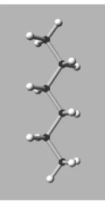
We are considering molecules made of carbon and hydrogen atoms (linear alkane), as shown on Fig. 2. The two extremal carbon atoms have three hydrogen atoms attached to them, while the others have two. The number of carbon atoms is a parameter.

These molecules are coded by the class CarbonChain. The following method builds a carbon chain with cNum carbon atoms:

Figure 2: Carbon chain (6 carbon atoms) p u b l i c void b u i l d ( ) 2 { b u i l d B a c k b o n e ( ) ; 4 addTop ( ) ; f o r _{( i n t k = 1 ; k < cNum−1; k++ ) addH2 ( k ) ;} 6 addBottom ( ) ; c r e a t e B o n d s ( ) ; 8 c r e a t e A n g l e s ( ) ; c r e a t e D i h e d r a l s ( ) ; 10 }

The backbone of carbon atoms is built by the call to buildBackbone. Meth-ods addTop and addBottom add 3 hydrogen atoms to the extremities of the molecule, and addH2 adds 2 hydrogens to each carbon, except the extremi-ties. The molecule components are created by the 3 methods createBonds, createAngles, and createDihedrals. The crucial point is that created molecules have an energy which is minimal. Minimality is obtained by placing atoms at positions compatibles with the potentials of the molecule components. Let us consider how this is done for the two hydrogens attached to each carbon, except the extremities. One first defines the (equilibrium) length lCH of bonds between carbon and hydrogen atoms, and the (equilibrium) valence angle aHCH between two hydrogens and one carbon atoms.

double lCH = bondC_H [ 1 ] ;

2 double aHCH = angleH_C_H [ 1 ] ;

double _{c o s = lCH ∗ Math . c o s (aHCH / 2 ) ;}

4 double s i n = lCH ∗ Math . s i n (aHCH / 2 ) ;

The addH2 method is defined by:

void addH2 ( i n t k ) 2 { Atom A = backbone [ k − 1 ] ; 4 Atom B = backbone [ k ] ; Atom C = backbone [ k + 1 ] ; 6 V e c t o r 3 d BA = U t i l s . v e c t (B,A ) ;

8 V e c t o r 3 d BC = U t i l s . v e c t (B, C ) ; V e c t o r 3 d P = U t i l s . n o r m a l i z e ( U t i l s . sum (BA,BC ) ) ; 10 V e c t o r 3 d N = U t i l s . n o r m a l i z e ( U t i l s . perp (BA,BC ) ) ; 12 V e c t o r 3 d u = U t i l s . extProd (− cos , P ) ; V e c t o r 3 d v = U t i l s . extProd (− s i n ,N ) ; 14 V e c t o r 3 d w = U t i l s . sum ( u , v ) ; V e c t o r 3 d q = U t i l s . sum ( u , U t i l s . o p p o s i t e ( v ) ) ; 16 Atom h1 = new H ( t h i s , U t i l s . sum (B . p o s i t i o n , w) ,B . v e l o c i t y ) ;

18 Atom h2 = new H ( t h i s , U t i l s . sum (B . p o s i t i o n , q ) ,B . v e l o c i t y ) ;

20 o t h e r s [ k ] = new Atom [ 2 ] ; o t h e r s [ k ] [ 0 ] = h1 ; 22 o t h e r s [ k ] [ 1 ] = h2 ; }

Atoms A,B,C are three successive carbon atoms, and B is the carbon on which two hydrogens have to be attached.

Two hydrogens atoms h1 and h2 are created and placed at their correct equilibrium positions. The two hydrogens are made accessible by the others array of B. By this construction, the two planes h1Bh2 and ABC are orthogonal, the angle h1Bh2 is equals to aHCH, and the distances h1B and h2B are both equal to lCH.

We now consider the creation of bonds. For the sake of simplicity, we do not consider the other components, which are processed in a similar manner. Bonds are created by the following method:

1 void c r e a t e B o n d s ( )

{

3 f o r _{( i n t k = 0 ; k < cNum − 1 ; k++ ) {}

new HarmonicBond ( t h i s , backbone [ k ] , backbone [ k + 1 ] ,bondC_C ) ; 5 } f o r ( i n t k = 0 ; k < cNum ; k++ ) { 7 Atom c = backbone [ k ] ; f o r ( i n t l = 0 ; l < o t h e r s [ k ] . l e n g t h ; l++ ) { 9 Atom a = o t h e r s [ k ] [ l ] ; i f ( a i n s t a n c e o f H ) 11 new HarmonicBond ( t h i s , c , a , bondC_H ) ;

e l s e i f ( a i n s t a n c e o f O )

13 new HarmonicBond ( t h i s , c , a , bondC_O ) ;

}

15 }

}

Lines 12-13 consider the case of oxygen atoms, to build acid molecules, which is not considerered here.

The molecule shown on Fig. 2 is made of 20 atoms, 19 bonds, 36 valence angles, and 45 dihedral angles.

5.4

Simulations

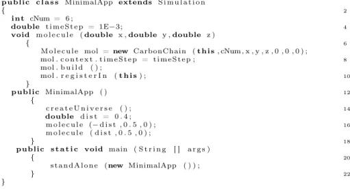
Reactive machines are basically provided by the class Simulation which extends the class Machine. An application can simply be defined as an extension of Simulation, as in:

p u b l i c c l a s s MinimalApp extends S i m u l a t i o n 2 { i n t cNum = 6 ; 4 double t i m e S t e p = 1E−3;

void m o l e c u l e ( double x , double y , double z )

6 {

M o l e c u l e mol = new CarbonChain ( t h i s , cNum , x , y , z , 0 , 0 , 0 ) ;

8 mol . c o n t e x t . t i m e S t e p = t i m e S t e p ; mol . b u i l d ( ) ; 10 mol . r e g i s t e r I n ( t h i s ) ; } 12 p u b l i c MinimalApp ( ) { 14 c r e a t e U n i v e r s e ( ) ; double d i s t = 0 . 4 ; 16 m o l e c u l e (− d i s t , 0 . 5 , 0 ) ; m o l e c u l e ( d i s t , 0 . 5 , 0 ) ; 18 } p u b l i c s t a t i c void main ( S t r i n g [ ] a r g s ) 20 { s t a n d A l o n e (new MinimalApp ( ) ) ; 22 } }

The number of carbon atoms cNum is set to 6 and the time-step is set to the femto-second (lines 3 and 4; the basic time unit of the system is the pico-second). A function which creates a molecule is defined lines 5-11. The molecule is built and registered in the simulation (which is denoted by this); the registration of the molecule entails the registration of all its components. The time-step of the created molecule is also set by the function. The constructor of the class is defined in lines 12-18. First, the createUniverse method provided by Java3D is called to initialise the graphics, then two molecules are created. The definition of the main Java method terminates the definition of the class MinimalApp.

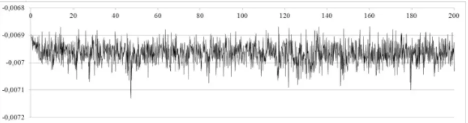
The intial state of the simulation is shown on left of Fig. 3 and the result after 50 ns (108

instants) is shown on the right. The evolution of the energy up to 200 ns (the internal energy unit is kg/mol × nm2

/ps2

) is shown on Fig. 4to illustrate the stability of the resolution (actually, stability has been tested up to one micro-second, that is 2.109

instants). The mean value is −6.97 × 10−3

with standard deviation 0.035 × 10−3_{. The energy is negative as result of the}

attraction due to van der Waals forces.

Figure 4: Evolution of energy during 200 ns

6

Related Work

The domain of physical simulations is huge and we shall thus only consider the use of reactive programming for implementing them, and the implementations of MD systems.

The application of reactive programming to newtonian physics has been initiated by Alexander Samarin in [17] where several 2D “applets” are proposed to illustrate the approach.

Cellular Automata (CA) have been used in several contexts of physics. The implementation of CA using a reactive programming formalism is described in [8].

In [9] is described a system that mimicks several aspects of quantum me-chanics (namely, self-interference, superposition of states, and entanglement). The system basically relies on a cellular automaton plunged into a reactive based simulation whose instants define the global time. Actually, this cannot be strictly speaking considered as a physical simulation but more as a kind of “proof of concept”.

A large number of MD simulation systems exist (for example [14] and [13], which are both open-source software). They are implemented in Fortran or C/C++. At the implementation level, the focus is put on real-parallelism and the use of multi-processor and/or multi-core architectures. On the contrary, we have choosen to use the Java language, and to put the focus more on expressivity than on efficiency, by using the logical parallelism of RP. We have adopted an open-source approach and integrated the 3D aspects directly in the system, by using Java3D.

7

Conclusion

We have shown that RP can be considered as a valuable tool for the implemen-tation of simulations in classical physics. We have illustated our approach by the description of a MD system [2] coded in RP. We plan to extend this MD system in several directions:

• _{Introduction of several multi-scale, multi-time-step aspects, building thus} a true MTMS system. Note that the dynamic creation/destruction pos-sibilities offered by RP will be central for the implementation of several notions (chimical reactions and reconstruction techniques, for example). • _{Use of real-parallelism. A first study has lead to the definition of a new}

version of SugarCubes (called SugarCubesv5 [3]) in which GPU-based ap-proaches become possible. The use of multi-processor machines should also of course be of great interest.

References

[1] Java3D. http://www.java3d.org.

[2] MDRP Site. http://mdrp.cemef.mines-paristech.fr.

[3] SugarCubesv5. http://cedric.cnam.fr/index.php/labo/membre/ view?id=160.

[4] Multiscale Simulation Methods in Molecular Sciences. NIC Series, Forschungszentrum Julich, Germany, vol. 42, Winter School, 2-6 March, 2009.

[5] A. C. T. van Duin, Siddharth Dasgupta, F. Lorant, and W. A. Goddard III. ReaxFF: A Reactive Force Field for Hydrocarbons. J. Phys. Chem. A, (105 (41)):pp 9396–9409, 2001.

[6] M. P. Allen and D. J. Tildesley. Computer Simulation of Liquids. Oxford, 1987.

[7] F. Boussinot. Reactive C: An Extension of C to Program Reactive Systems. Software Practice and Experience, 21(4):401–428, april 1991.

[8] F. Boussinot. Reactive Programming of Cellular Automata. Technical Report RR-5183, INRIA, May 2004.

[9] F. Boussinot. Mimicking Quantum Mechanics Using Reactive Program-ming. International Journal of Modern Physics C, 22(06):635–648, 2011. [10] F. Boussinot and J-F. Susini. The SugarCubes Tool Box - A Reactive Java

Framework. Software Practice and Experience, 28(14):1531–1550, december 1998.

[11] W. Damm, A. Frontera, J. Rirado-Rives, and W. L. Jorgensen. OPLS All-Atom Force Field for Carbohydrates. Journal of Computational Chemistry, 18(16):1955–1970, 1997.

[12] D. Knuth. The Art of Computer Programming. Addison-Wesley, 1968. [13] Sandia National Laboratory. LAMMPS.

[14] STFC Daresbury Laboratory. DL_POLY.http://www.cse.scitech.ac. uk/ccg/software/DL_POLY.

[15] L. Mandel and M. Pouzet. ReactiveML, A Reactive Extension to ML. In ACM International conference on Principles and Practice of Declarative Programming (PPDP’05), Lisbon, Portugal, July 2005.

[16] B. Monasse and F. Boussinot. Determination of Forces from a Potential in Molecular Dynamics. ArXiv e-prints http: // arxiv. org/ abs/ 1401. 1181, January 2014.

[17] A. Samarin. Application de la programmation réactive à la modélisation en Physique. Rapport de stage de DEA, UNSA, 2002, http://www-sop. inria.fr/mimosa/rp_2004/SimulationInPhysics.

[18] L. Verlet. Computer "Experiments" on Classical Fluids. I. Thermodynam-ical Properties of Lennard-Jones Molecules. Phys. Rev., 159:98–103, Jul 1967.