HAL Id: hal-00721335
https://hal.archives-ouvertes.fr/hal-00721335
Submitted on 27 Jul 2012
HAL is a multi-disciplinary open access
archive for the deposit and dissemination of
sci-entific research documents, whether they are
pub-lished or not. The documents may come from
teaching and research institutions in France or
abroad, or from public or private research centers.
L’archive ouverte pluridisciplinaire HAL, est
destinée au dépôt et à la diffusion de documents
scientifiques de niveau recherche, publiés ou non,
émanant des établissements d’enseignement et de
recherche français ou étrangers, des laboratoires
publics ou privés.
Memory Bounds for the Distributed Execution of a
Hierarchical Synchronous Data-Flow Graph
Karol Desnos, Maxime Pelcat, Jean François Nezan, Slaheddine Aridhi
To cite this version:
Karol Desnos, Maxime Pelcat, Jean François Nezan, Slaheddine Aridhi. Memory Bounds for the
Distributed Execution of a Hierarchical Synchronous Data-Flow Graph. 12th International Conference
on Embedded Computer Systems: Architecture, Modeling and Simulation (SAMOS XII), Jul 2012,
Agios Konstantinos, Greece. pp.160. �hal-00721335�
Memory Bounds for the Distributed Execution of a
Hierarchical Synchronous Data-Flow Graph
Karol Desnos, Maxime Pelcat, Jean-Francois Nezan
IETR, INSA Rennes, CNRS UMR 6164, UEB 20, Av. des Buttes de Co¨esmes, 35708 Rennes email: kdesnos, mpelcat, [email protected]Slaheddine Aridhi
Texas Instruments France 06271 Villeneuve Loubet, Franceemail: [email protected]
Abstract—This paper presents an application analysis tech-nique to define the boundary of shared memory requirements of Multiprocessor System-on-Chip (MPSoC) in early stages of devel-opment. This technique is part of a rapid prototyping process and is based on the analysis of a hierarchical Synchronous Data-Flow (SDF) graph description of the system application. The analysis does not require any knowledge of the system architecture, the mapping or the scheduling of the system application tasks.
The initial step of the method consists of applying a set of transformations to the SDF graph so as to reveal its memory characteristics. These transformations produce a weighted graph that represents the different memory objects of the application as well as the memory allocation constraints due to their relationships. The memory boundaries are then derived from this weighted graph using analogous graph theory problems, in particular the Maximum-Weight Clique (MWC) problem. State-of-the-art algorithms to solve these problems are presented and a heuristic approach is proposed to provide a near-optimal solution of the MWC problem. A performance evaluation of the heuristic approach is presented, and is based on hierarchical SDF graphs of realistic applications. This evaluation shows the efficiency of proposed heuristic approach in finding near optimal solutions.
I. INTRODUCTION
During the design of an embedded system, the treatment of memory issues strongly impact the final system quality and performance, as the area occupied by the memory can be as large as 80% of the chip and may be responsible for a major part of its power consumption [1]. Prior work on memory issues for Multiprocessor System-on-Chip (MPSoC) mostly consists of optimization techniques that minimizes the amount of memory allocated to run an application, thus reducing the capacity and area of memory of the developed system [2], [3], [4]. These techniques rely on a precise knowledge of system behavior, particularly scheduling and mapping the application tasks on the system processors, and so may only be applied during late stages of the system design process.
The purpose of the method presented in this paper is to derive the memory bound requirements of a system (Figure 1) in the early stages of its development when there is a complete abstraction of the system architecture. This method is based on an analysis of the system application, and allows the developer of a multi-core shared-memory system to adequately size the chip memory.
This paper focuses on memory characterization of applica-tions described by a Dataflow Process Network (DPN) Model
of Computation (MoC) [5]. A MoC defines the semantics of an algorithm model: which components the model can contain, how they are interconnected and how they interact. A DPN MoC divides the application into computational entities named actors that exchange data via First-In First-Out (FIFO) channels. The algorithm model is specified as a directed application graph in which nodes represent actors and edges represent FIFO queues. Each actor is associated to firing rules specifying its behavior in terms of token consumption and production. Tokens are abstract representations of a data quantum, independent of its size. The actors themselves are “black boxes” of the model and may be implemented in any programming language. Firing an actor consists of starting its preemption free execution.
The Synchronous Data-Flow (SDF) MoC is certainly the most widely used DPN model. It consists of a static model in which all production and consumption token rates are fixed and known at compile time. This property makes the model analysis possible at compile time. Interface Based SDF (IBSDF) is a hierarchical DPN MoC based on SDF that can be analyzed hierarchically [6].
Insufficient
memory allocated memoryPossible memoryWasted
Available Memory Maximum-Weight Clique Problem Heuristic for Maximum-Weight Clique Problem
≤
≤
Interval Coloring Problem Sum of vertices weights 0 Insufficientmemory allocated memoryPossible memoryWasted
Available Memory Lower Bound= Optimal Allocation Upper Bound= Worst Allocation 0
Fig. 1. Memory Bounds
The rapid prototyping context and the IBSDF model, which serves as an input to our method, are introduced in section II and the successive transformations applied to the application graph to reveal its memory characteristics are developed in section III. Then, section IV presents existing algorithms and a new heuristic approach to derive the memory bounds of an application. An overview of previous research on memory is-sues for multi-core systems is given in section V. Finally, after an evaluation of the performance of our method in section VI, we conclude this paper and propose possible directions for future work in section VII.
In Proceedings of the International Conference on Embedded Computer
Systems: Architecture, Modeling and Simulation (SAMOS), 2012.
II. CONTEXT
A. Interface-Based Synchronous Data-Flow Graph
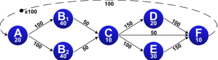
IBSDF [6] is a static hierarchical dataflow MoC defined as an extension of SDF. Figure 2 shows an example of an IBSDF graph, where the top level comprises 3 actors A, B and hthat respect the SDF semantics. Edges are labeled with their token production and consumption rates. An edge with a black dot signifies that initial tokens are present in the FIFO queue when the system starts to execute. The number of initial tokens is specified by the x100 label. Initial tokens are a semantic element of the SDF MoC that makes communication possible between successive iterations of the graph execution. h is an IBSDF hierarchical actor. Its behavior is given by a subgraph containing source and sink interfaces. These interfaces insulate the behavior of the top graph and subgraph. This property makes the algorithm description process simpler and less error-prone [6].
A
20C
10F
10E
30D
20B
401B
2 40 150 100 150 100 100 100 50 50 50 100 x100A
20B
40C
10F
10E
30D
20 200 100 50 100 150 150 100 100 150 150 100 100 50 50 100 100 x100A
20 200 100B
40 50 100 100 100C
10F
10E
30D
20 150 150 100 100 150 150 100 100 50 50 Source Sink 100 100h
x100AB
1002AB
1 100CE
100CD
150CF
50EF
150DF
100B
1C
50B
2C
50Fig. 2. Interface Based SDF (IBSDF) graph
Like SDF, IBSDF is an untimed MoC. It specifies actor dependencies but does not take into account the time needed to execute the actors. The memory bounds presented in this paper are thus computed without actor timing consideration and, in that sense, characterize an application IBSDF graph independent of implementation. This is in contrast to the related work from the literature, which tends to focus on post-scheduling and execution timing analysis (see Section V). B. Hardware/Software Exploration Workflow
Rapid prototyping consists of extracting information from a system in the early stages of its development. It enables hardware/software co-design and favors early decisions that improve system architecture efficiency. The work presented in this paper aims to extract memory information from an application graph at an early stage of system design and inde-pendent of architecture details. It allows the system designer to discard architectures with insufficient memory and to evaluate the degree of memory optimization required to produce the final system with an optimal amount of memory.
Figure 3 illustrates the position of the memory bounds computation in the rapid prototyping process as proposed in [7]. Rapid prototyping inputs consist of an algorithm model respecting the IBSDF MoC, an architecture model respecting the System-Level Architecture Model (S-LAM) semantics
Rapid Prototyping IBSDF Algo S-LAM Archi Scenario Algo Transfos Archi Transfos Scheduling Simulation Code Generation Exporting Results Memory Bounds Computation DAG
Fig. 3. Rapid Prototyping Process
[8] and a scenario providing constraints and prototyping parameters. The scenario ensures the complete separation of algorithm and architecture models. Algorithm and architecture models undergo transformations in preparation for the rapid prototyping steps. Static multi-core scheduling is then applied to dispatch the algorithm actors to the architecture processing elements and to schedule their executions [9] [10]. Finally, the scheduling information is used to simulate the system behavior and to generate compilable code for the targeted architecture. It can also be exported to an external SystemC based simulator. In this process, the memory bounds computation is executed on the transformed algorithm graph and has no dependency on the architecture graph. The next section explains the IBSDF graph properties and Section III-A details the algorithm transformations applied to IBSDF prior to the memory bounds computation.
III. PREPROCESSING TOWARDMEMORYANALYSIS
A. Algorithm Transformations
The first step to characterize the memory bounds of an application consists of applying a set of transformations to its IBSDF Graph. The SDF model of the application is successively flattened, and first converted into a Single Rate SDF, then into a Directed Acyclic Graph (DAG). As presented in [6], these transformations are used to reveal the parallelism embedded in the IBSDF model, thus enabling a better mapping and scheduling of its actors on a multicore architecture.
A
20C
10F
10E
30D
20B
401B
402 150 100 150 100 100 100 50 50 50 100 x100A
20B
40C
10F
10E
30D
20 200 100 50 100 150 150 100 100 150 150 100 100 50 50 100 100 x100A
20 200 100B
40 50 100 100 100C
10F
10E
30D
20 150 150 100 100 150 150 100 100 50 50 Source Sink 100 100h
x100AB
1002AB
1 100CE
100CD
150CF
50EF
150DF
100B
1C
50B
2C
50Fig. 4. Flattened Synchronous Data-Flow
To illustrate these transformations, we successively apply them to the IBSDF graph of Figure 2. The first transformation consists of flattening the hierarchy of the graph by replacing all hierarchical nodes with their content. The IBSDF graph is thus transformed into a SDF graph presented in Figure 4.
The second transformation is the conversion into a Single-Rate SDF graph: a SDF where the production and consumption values on each edge are equal. In this model, each vertex corresponds to a single actor firing from the SDF graph. This conversion is performed by computing the topology matrix [11], multiplying actors by the number of their firings and reorganizing edges, as shown in Figure 5, where actor B is split in two instances. An algorithm to perform this conversion can be found in [12].
The last conversion consists of generating an acyclic prece-dence graph by isolating one iteration of the algorithm. This is achieved by ignoring the edges with initial tokens in the single-rate SDF. In our example, this transformation results in ignoring the feedback edge F→A which stores 100 initial tokens.
A
20C
10F
10E
30D
20B
401B
402 150 100 150 100 100 100 50 50 50 100 x100A
20B
40C
10F
10E
30D
20 200 100 50 100 150 150 100 100 150 150 100 100 50 50 100 100 x100A
20 200 100B
40 50 100 100 100C
10F
10E
30D
20 150 150 100 100 150 150 100 100 50 50 Source Sink 100 100h
x100AB
1002AB
1 100CE
100CD
150CF
50EF
150DF
100B
1C
50B
2C
50Fig. 5. Single-Rate SDF or Directed Acyclic Graph if dotpoint edge ignored
In the context of memory analysis, these transformations are applied to fulfill the following objectives:
• Expose data parallelism: Concurrent analysis of data parallelism and data precedence gives information on the lifetime of memory objects prior to any scheduling step. Indeed, two FIFO queues belonging to parallel data-paths may contain data tokens simultaneously and consequently are forbidden from sharing a memory space. Conversely, two FIFOs linked with a precedence constraint, such as A→B and C→F FIFOs in Figure 4, will never store data tokens simultaneously, thus can share the same memory space.
• Break FIFOs into buffers shared between actors: In the
SDF model, the channels carrying data tokens between actors behave like FIFO queues. The memory needed to allocate each FIFO corresponds to the maximum number of tokens stored during an execution of the graph. As this number of tokens depends on the schedule of the actors, methods exist to derive a schedule that minimizes the memory needed to allocate the FIFOs [13]. However, in our method, the memory analysis is not dependent on scheduling considerations. It is for this reason that FIFOs of undefined sizes before the scheduling step are replaced with buffers of fixed sizes during the transformation of the graph into a single-rate SDF. In Figure 5, buffers linking two actors will be written and read only once with a data token of fixed size, which simplifies the memory analysis.
• Derive an acyclic model:Cyclic data-paths in an IBSDF
graph are an efficient way to model iterative or recursive calls to a subset of actors. In order to use efficient static scheduling algorithms [14], SDF models are often
converted into DAGs before being scheduled. Besides revealing data-parallelism, this transformation makes it easier to schedule an application, as each actor is fired only once per execution of the resulting DAG. Similarly, in the absence of a schedule, deriving a DAG permits the use of memory objects (communication buffers) that will be written and read only once per execution of the DAG. Consequently, before a memory object is written and after it is read, its memory space will be reusable to store another object.
B. Memory objects
The DAG resulting from the transformations of an IBSDF graph, contains three types of memory objects
• Communication buffers: The first type memory object corresponds to the directed edges of the DAG and are the buffers used to transfer data between consecutive actors. In our approach, we consider that the memory allocated to these buffers is reserved from the execution start of the edge producer actor until the completion of the edge consumer actor. This choice is made to enable custom token consumption throughout actor firing time. As a consequence, the memory used to store an input buffer of an actor should not be reused to store an output buffer of the same actor. In Figure 5, the 150 units of memory used to carry data between actors C and D can not be reused, even partially, to transfer data from D to F.
• Working memory of actors:This second type of memory object is the maximum amount of memory allocated by an actor during its execution. This working memory represents the memory needed to store the data used during the computations of the actor but does not include the input nor the output buffers memory. In our method, we assume that an actor keeps an exclusive access to its working memory during its execution. In Figures 2 to 5, the size of the working memory associated with each actor is given by the number below the actor name. This memory is equivalent to a task stack space in an operating system.
• Feedback FIFOs:The final type of memory object corre-sponds to the memory needed to store edges ignored as a result of the transformation of a Single-Rate SDF into a DAG. These edges which are ignored to break cycles, can still carry data between successive executions of the DAG and behave like FIFO queues. These feedback edges may not share memory space with any other memory object of the application.
C. Memory Exclusion Graph
Once an application has been transformed into a DAG, and all its memory objects have been identified, the last pre-processing step of our method consists of deriving the memory exclusion graph which will serve as a basis to our analysis.
A memory exclusion graph is an undirected weighted graph denoted by G =< V, E, w > where:
• V is the set of vertices. Each vertex represents an indivisible memory object.
• E is the set of edges representing the memory exclusions. • w : V → N is a function with w(v) the weight of a
vertex v. The weight of a vertex corresponds to the size of the associated memory object.
We also denote:
• N (v) the neighborhood of v, i.e. the set of vertices linked
to v by an edge. Vertices of this set are said to be adjacent to v.
• |S| the cardinality of a set S. |V | and |E| are thus
respectively the number of vertices and edges of the graph.
• δ(G) = |V |·(|V |−1)2·|E| the edge density of the graph cor-responding to the ratio of existing edges to all possible edges.
A
20C
10F
10E
30D
20B
1 40B
402 150 100 150 100 100 100 50 50 50 100A
20B
40C
10F
10E
30D
20 200 100 50 100 150 150 100 100 150 150 100 100 50 50 100 100A
20 200 100B
40 50 100 100 100C
10F
10E
30D
20 150 150 100 100 150 150 100 100 50 50 Source Sink 100 100h
AB
1002AB
1001CE
100CD
150CF
50EF
150DF
100B
1C
50B
2C
50Fig. 6. Memory Exclusion Graph
Two memory objects of any type exclude each other (i.e. they can not share the same memory space) if a schedule can be derived from the DAG where both these memory objects store data simultaneously. Some exclusions are directly caused by the properties of the memory objects, such as exclusions between input and output buffers of an actor. Other exclusions result from the parallelism of an application, as is the case with the working memory of actors from parallel data-paths that might be executed concurrently.
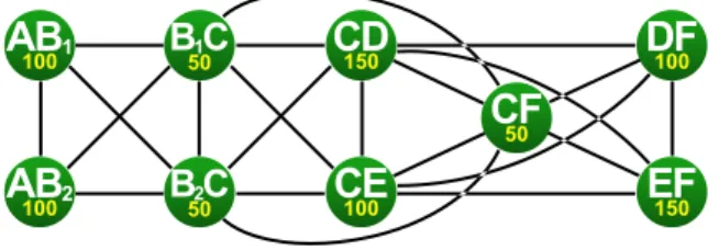
The memory exclusion graph presented in Figure 6 is de-rived from the IBSDF graph of Figure 2. The complete graph contains 17 memory objects and 66 exclusions but, for clarity, only the vertices corresponding to the buffers between actors (type 1) are presented.
Building a memory exclusion graph based on a DAG consists of scanning its actors and data-transfers in order of precedence, so as to identify its parallel branches. As part of this scan, the memory objects and the exclusions caused by a precedence relationship are added to the memory exclusion graph. The, exclusions are then inserted between all memory objects which have been identified in the DAG as belonging to parallel branches. An alternative way of building an exclusion graph is to first build its complement graph, within which two vertices are linked if the corresponding memory objects can share a memory space. Then, the exclusion graph is simply obtained by considering that two of its vertices are linked if they are not connected by an edge in the complement graph. In our method, the memory exclusion graph is built based on a non-scheduled DAG allowing the characterization of the
application independent of architecture constraint. However, a subsequent update of this graph to incorporate the changes resulting from a schedule is possible. Indeed, a static schedule introduces an execution order of the graph actors, which can be seen as a new precedence relationship between actors. The addition of this new precedence link to a DAG, results in the possible disappearance of a certain amount of parallelism and the resulting exclusions. For example in Figure 5, if actor D is scheduled before actor E, then the exclusion disappears be-tween the working memory of D and the E→F communication buffer.
IV. MEMORYALLOCATIONBOUNDS
The upper and lower bounds of the static memory allocation of an application are respectively a maximum and a minimum limit to the amount of memory needed to run an application, as presented in Figure 1. These bounds are crucial information in the co-design process, as they allow the developer to adjust the size of the memory available accordingly to the application requirements. Furthermore, as these bounds can be computed during the early development of a MPSoC, they might prevent the developer from mapping an insufficient or an unnecessarily large memory chip.
A. Least upper bound
The least upper memory allocation bound of an application corresponds to the size of the memory needed to allocate each memory object in a dedicated memory space. Such an allocation would be a waste of memory, as a memory space used to store an object would never be reused to store another. However, this allocation scheme must be used for exclusion graphs where an exclusion exists for every pair of vertices.
Given an exclusion graph G, its upper memory allocation bound is thus the sum of the weight of its vertices:
BoundM ax(G) =
X
v∈V
w(v) (1)
The upper bound for the exclusion graph of Figure 6 is 850 units, and the upper bound for the complete exclusion graph derived from the IBSDF of Figure 2 is 1020 units. B. Greatest lower bound
The greatest lower memory allocation bound of an appli-cation is the least amount of memory required to execute it. Finding this optimal allocation based on an exclusion graph can be done by solving the equivalent Interval Coloring Problem [15], [3].
A k-coloring of an exclusion graph is the association of each vertex vi of the graph with an interval Ii = {a, a +
1, · · · , b − 1} of consecutive integers - called colors -, such that b − a = w(v). Two distinct vertices vi and vj linked
by an edge must be associated to non-overlapping intervals. Assigning an interval to a weighted vertex is equivalent to allocating a range of memory address to a memory object. Consequently, a k-coloring of an exclusion graph corresponds to an allocation of its memory objects.
The Interval Coloring Problem consists of finding a k-coloring of the exclusion graph with the fewest integers used in the Ii intervals. This objective is equivalent to finding
the allocation of memory objects that uses the least memory possible, thus giving the greatest lower bound of the memory allocation.
Unfortunately, as presented in [15], this problem is known to be NP-Hard, therefore it would be prohibitively long to solve in the rapid prototyping context which involves applications with hundreds or thousands of buffers. Moreover, a sub-optimal solution to the Interval Coloring problem corresponds to an allocation that uses more memory than the minimum possible: more memory than the greatest lower bound. Conse-quently, a sub-optimal solution fails to achieve our objective which is to find a lower bound to the size of the memory allocated for a given application.
Insufficient
memory allocated memoryPossible memoryWasted
Available Memory Maximum-Weight Clique Problem Heuristic for Maximum-Weight Clique Problem
≤
≤
Interval Coloring Problem Sum of vertices weights 0 Insufficientmemory allocated memoryPossible memoryWasted
Available Memory Lower Bound = Optimal Allocation Upper Bound = Worst Allocation 0
Fig. 7. Memory Bounds
C. Lower bound using exact solution to the Maximum-Weight Clique Problem
Since the greatest lower bound can not be found in reason-able time, we focus our attention on finding a lower bound close to the size of the optimal allocation. In [3], Fabri introduces another lower bound derived from an exclusion graph: the weight of the Maximum-Weight Clique (MWC).
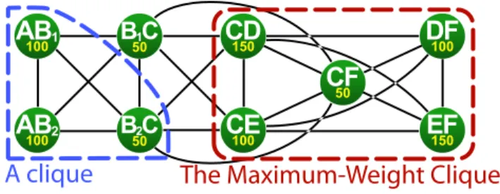
A clique is a subset of vertices that forms a subgraph within which each pair of vertices is linked with an edge. As memory objects of a clique can not share memory space, their allocation requires a memory as large as the sum of the weights of the clique elements, also called the clique weight. The subsets {CD,CE,CF,DF,EF} or {AB1,AB2,B2C} are examples
of cliques in the exclusion graph of Figure 8. Their respective weights are 550 and 250. By definition, a single vertex can also be considered as a clique, and a clique is called maximal if no vertex can be added to it to form a larger clique. In Figure 8, clique {CD,CE,CF,DF,EF} is maximal, but {AB1,AB2,B2C}
is not as B1C is linked to all the clique vertices and can
therefore be added to the clique.
The Maximum-Weight Clique (MWC) of a graph is the clique whose weight is the largest of all cliques in the graph. Although this problem is also known to be NP-Hard, several branch-and-bound algorithms have been proposed to solve it efficiently. In [16], ¨Osterg˚ard proposes an exact algorithm which is, to our knowledge, the fastest algorithm for exclusion graphs with an edge density under 0.80. For graphs with an edge density above 0.80, a more efficient algorithm was
A
20C
10F
10E
30D
20B
401B
402 150 100 150 100 100 100 50 50 50 100 x100A
20B
40C
10F
10E
30D
20 200 100 50 100 150 150 100 100 150 150 100 100 50 50 100 100 x100A
20 200 100B
40 50 100 100 100C
10F
10E
30D
20 150 150 100 100 150 150 100 100 50 50 Source Sink 100 100h
x100AB
2 100AB
1001CE
100CD
150CF
50EF
150DF
100B
1C
50B
2C
50AB
1002AB
1001CE
100CD
150CF
50EF
150DF
100B
1C
50B
2C
50The Maximum-Weight Clique
A clique
Fig. 8. Clique examples
proposed by Yamaguchi et al in [17]. Both algorithms are recursive and use a similar approach: beginning with a single vertex, they search for the MWC Ci in a subset of the graph,
then add a vertex to the considered subset and use the weight of Ci to bound the search for a larger clique Ci+1in the new
subgraph. The two algorithms were implemented in order to compare their performances on exclusion graphs derived from different applications (cf. section VI).
In the exclusion graph of Figure 8, the MWC is {CD,CE,CF,DF,EF} with a weight of 550 units.
The weight of the MWC corresponds to the amount of memory needed to allocate the memory objects belonging to this subset of the graph. By extension, the allocation of the whole graph will never use less memory than the weight of its MWC. Therefore, this weight is a lower bound to the memory allocation and is less than or equal to the greatest lower bound, as shown in Figure 7.
D. Lower bound using approximate solution to the Maximum-Weight Clique Problem
¨
Osterg˚ard’s and Yamaguchi’s algorithms are exact algo-rithms and not heuristics. As the MWC problem is an NP-Hard problem, and even using these fast algorithms, an exact solution in polynomial time can not be guaraneed. In the rapid prototyping context, all methods and algorithms used must have a short and predictable runtime; that is why we developed a heuristic algorithm for the MWC problem.
The proposed heuristic approach, presented in Figure 9, is an iterative algorithm whose basic principle is to remove a ju-diciously selected vertex at each iteration, until the remaining vertices form a clique.
Our algorithm can be divided into 3 parts:
• Initializations (lines 1-5): For each vertex of the graph, the cost function is initialized with the weight of the vertex summed with the weights of its neighbors. In order to keep the input graph unaltered through the algorithm execution, its set of vertices V and its number of edges |E| are copied in local variables C and nbedges. • Algorithm core loop (lines 6-13):During each iteration of
this loop, the vertex with the minimum cost v∗is removed from C (line 8). In few cases where several vertices have the same cost, the lowest number of neighbor |N (v)| then the smallest weight w(v) are used to determine the vertex to remove. By doing so, less edges are removed from the graph and the edge density of remaining vertices will be
Input: a memory exclusion graph G =< V, E, w > Output: a maximal clique C
1: C ← V 2: nbedges ← |E| 3: for each v ∈ C do 4: cost(v) ← w(v) +P v0∈N (v)w(v0) 5: end for
6: while |C| > 1 and |C|·(|C|−1)2·nbedges < 1.0 do 7: Select v∗ from V that minimizes cost(·)
8: C ← C \ {v∗} 9: nbedges← nbedges− |N (v∗) ∩ C| 10: for each v ∈ N (v∗) ∩ C do 11: cost(v) ← cost(v) − w(v∗) 12: end for 13: end while
14: Select a vertex vrandom∈ C 15: for each v ∈ N (vrandom) \ C do 16: if C ⊂ N (v) then
17: C ← C ∪ {v}
18: end if
19: end for
Fig. 9. Maximum-Weight Clique Heuristic Algorithm
higher, which is desirable when looking for a clique. If there still are multiple vertices with equal properties, a random vertex is selected among them.
This loop is iterated until the vertices in subset C become a clique. This condition is checked line 6, by comparing 1.0 - the edge density of a clique - with the edge density of the subgraph of G formed by the remaining vertices in C. To this purpose nbedge, the number of edges of this
subgraph, is decremented line 9 by the number of edges in E linking the removed vertex v∗to vertices in C. Lines 10 to 12, the costs of the remaining vertices are updated for the next iteration.
• Clique maximization (lines 14-19): This last part of the algorithm ensures that the clique C is maximal by adding neighbor vertices to it. To become a member of the clique, a vertex must be adjacent to all its members. Consequently, the candidates to join the clique are the neighbors of a vertex randomly selected in C. If a vertex among these candidates is linked to all vertices in C, it is added to the clique.
The complexity of this heuristic algorithm is of the order of O(|N |2), where |N | is the number of vertices of the exclusion graph.
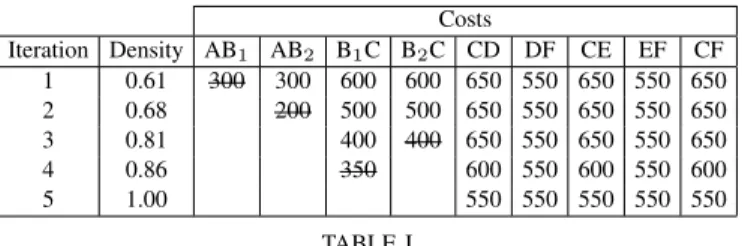
For example, in Table I, the algorithm is applied to the exclusion graph of Figure 6. For each iteration, the costs of the remaining vertices are given, and the vertex removed during the iteration is crossed out. The column Density corresponds to the edge density of the subgraph formed by the remaining vertices.
In this simple example, the clique found by the heuristic algorithm and the exact algorithm are the same, and their
Costs Iteration Density AB1 AB2 B1C B2C CD DF CE EF CF 1 0.61 300 300 600 600 650 550 650 550 650 2 0.68 200 500 500 650 550 650 550 650 3 0.81 400 400 650 550 650 550 650 4 0.86 350 600 550 600 550 600 5 1.00 550 550 550 550 550 TABLE I
ALGORITHM PROCEEDING FOR EXCLUSION GRAPH OFFIGURE6
weight also corresponds to the size of the optimal allocation. This example proves that, as shown in Figure 7, the result of the heuristic can be equal to the exact solution of the MWC problem, whose size can also equal the size of the optimal allocation.
V. RELATEDWORKS
To the extent of our knowledge, memory optimization for multi-core systems has generally been studied in the literature as a post-scheduling process. Using the scheduling information, the lifetimes of the different memory objects of an application are derived. Minimization is then achieved by allocating several memory objects whose lifetimes do not overlap in the same memory space.
Once the lifetimes of the memory objects are obtained, the memory allocation is performed using one of these different approaches:
• Running static - or offline - allocation algorithms inspired by dynamic allocators, such as those proposed in [1], [4], [2]. As opposed to dynamic allocators which allocate memory objects in order they are brought to them, static allocators have a global knowledge of all memory ob-jects at compile time, thus making further optimizations possible.
• Coloring an exclusion graph that models the conflicting memory objects [15], [4]. An equivalent approach is to use the complement graph, where memory objects are linked if they have non-overlapping lifetime, and perform a clique partitioning of its vertices [18].
• Using constraint programming, as is the case in [19] where memory constraints are used together with cost, resource usage and execution time constraints.
Besides the post-scheduling techniques, a few publications also consider the memory optimizations during the scheduling process. In [2], [13], algorithms are presented to derive a schedule from a SDF graph so that the size of the FIFOs between actors is minimized. Another technique proposed in [20], consists of iterating the scheduling and the memory allocation steps and keeping only the schedule whose corre-sponding memory allocation uses the least memory.
Finally, certain optimization techniques can be applied before the scheduling step. These techniques mostly consist of modifying the description of the application behavior so as to maximize the impact of later optimizations. Variable renaming, instruction re-ordering, loop merging and splitting
are examples of modifications for imperative languages that can reduce the memory needs of an application [3]. Similar modifications can be applied to SDF graphs, as was done in [6] where a technique used to extract parallelism from nested loops in imperative languages is adapted to reveal data parallelism embedded in an IBSDF graph.
As explained in [21], the former optimization techniques often require a partial system synthesis and the execution of time-consuming algorithms. Although these techniques pro-vide an exact or highly optimized memory requirement, they may be too slow to be used in the rapid prototyping context. In [21], Balasa et al. survey existing estimation techniques that provide a reliable memory size approximation in a reasonable computation time. The main difference between these estima-tion techniques and our bounding method is the abstracestima-tion level considered. Indeed, these techniques are mostly based on the analysis of imperative code while our method deals with applications modeled with SDF graphs.
VI. RESULTS
The memory bounds are computed in the PREESM1 rapid prototyping framework [7]. PREESM is an open-source Eclipse-based tool providing graph transformation algorithms, multi-core scheduling and C code generation from IBSDF graphs. Algorithms for memory bound computation have been implemented in Java in this framework. All results presented in this section are obtained by running the algorithms on a 3.1GHz CPU.
Graphs properties Exact algorithms Heuristic |V | δ(G) Osterg˚ard’s Yamaguchi’s¨ Time Efficiency
60 0.80 0.05 s 0.25 s 0.004 s 91% 80 0.80 0.43 s 2.04 s 0.009 s 89% 100 0.80 3.4 s 11.73 s 0.014 s 87% 120 0.80 17.93 s 55.23 s 0.024 s 86% 60 0.90 0.35 s 0.56 s 0.004 s 94% 80 0.90 9.34 s 7.83 s 0.009 s 93% 100 0.90 188.00 s 90.90 s 0.016 s 91%
Efficiency: Ratio of the size of the clique found by the heuristic algorithm over the size of the maximum weight clique
TABLE II
PERFORMANCE OFMAXIMUM-WEIGHTCLIQUE ALGORITHMS ON RANDOM EXCLUSION GRAPHS
Table II shows the performance of different algorithms for the MWC problem. Each entry presents the mean performance obtained from 400 randomly generated exclusion graphs with a fixed number of vertices (|V |) and a fixed density of edges (δ(G)). For each exclusion graph, the weights of its vertices are uniformly distributed in a predefined range. The 400 graphs are generated with ranges varying from [1000; 1010] to [1000; 11000]. Columns ¨Osterg˚ard’s, Yamaguchi’s and Time respectively give the mean runtime of each of the three algorithms, and the Efficiency column gives the average ratio of the clique size found by the heuristic algorithm over the size of the MWC.
1PREESM project: http://sourceforge.net/projects/preesm/
It should be noted that the clique maximization part of the heuristic algorithm was deactivated in all tests of this section. Indeed, several tests showed that this maximization improved the mean efficiency by only 2%, while multiplying the runtime of the heuristic by a factor 1,6.
Table II shows that the runtime of exact algorithms grows exponentially with the number of nodes of the exclusion graphs, and is highly dependent on the edge density of the graphs. Conversely, the runtime of the heuristic algorithm is roughly proportional to |V |2 and is not strongly influenced
by the edge density of the graphs. The results in table II also reveal that the mean efficiency of the heuristic algorithm for random exclusion graphs is of the order of 90%, and decreases slightly as the number of vertices increases. Finally, these results additionally confirm that Yamaguchi’s algorithm has better performance than ¨Osterg˚ard’s algorithm for graphs with more than 80 vertices and an edge density higher than 0,80.
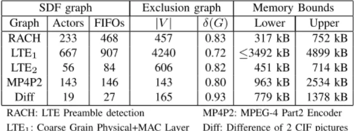
SDF graph Exclusion graph Memory Bounds Graph Actors FIFOs |V | δ(G) Lower Upper RACH 233 468 457 0.83 317 kB 752 kB
LTE1 667 907 4240 0.72 ≤3492 kB 4899 kB
LTE2 56 84 606 0.82 451 kB 714 kB
MP4P2 143 146 143 0.80 963 kB 2534 kB Diff 19 27 165 0.93 779 kB 1378 kB RACH: LTE Preamble detection MP4P2: MPEG-4 Part2 Encoder LTE1: Coarse Grain Physical+MAC Layer Diff: Difference of 2 CIF pictures
LTE2: Coarser Grain Physical+MAC Layer
TABLE III
PROPERTIES OF THE TEST GRAPHS
The performance of each of the three algorithms was also tested using exclusion graphs derived from IBSDF graphs of functional applications. Table III shows the characteristics of the tested graphs. The first three entries of this table, namely RACH, LTE1 and LTE2, correspond to application graphs
describing parts of the Long Term Evolution (LTE) wireless communication standard. The last two entries, MP4P2 and Diff, respectively, are a description of the MPEG-4 (Moving Picture Experts Group) Part2 video encoder, and a dummy application that computes the difference between successive video frames. The values given for Actors and FIFOs are those of the flattened IBSDF graph, before its conversion into a DAG. It may also be noted that the lower memory bound indicated in Table III corresponds to the size of the MWC. In this section, only the memory objects corresponding to the communication buffers (type 1) were considered to generate the exclusion graphs.
To take advantage of a multi-core architecture, an applica-tion modeled with an SDF graph must present a high degree of parallelism. Exclusion graphs derived from such applications will therefore have a high edge density, as is the case with the graphs of Table III. The performance of each of the three algorithms on these graphs are related in Table IV.
As shown in Table IV, the efficiency of the heuristic al-gorithm for exclusion graphs derived from real applications is much higher than for randomly generated exclusion graphs.
In-Exact algorithms Heuristic Graph Osterg˚ard’s Yamaguchi’s¨ Time Efficiency RACH ∞ 207.00 s 1.200 s 99.9% LTE1 ∞ ∞ 869.320 s - % LTE2 996.70 s 219.60 s 3.300 s 100.0% MP4P2 1.12 s 0.50 s 0.052 s 99.9% Diff 0.42 s 0.49 s 0.120 s 100.0% TABLE IV
PERFORMANCE OFMAXIMUM-WEIGHTCLIQUE ALGORITHMS ON EXCLUSION GRAPHS DERIVED FROM THE TEST GRAPHS
deed, the heuristic algorithm always finds a clique with weight almost equal to the weight of the MWC and has a runtime at least 4 times faster. Moreover, contrary to the exact algorithms which sometimes fail to find a solution within 12 hours (as denoted by ∞), the runtime of the heuristic algorithm is highly predictable as it is solely dependent on the number of memory objects |V |. In the case of LTE1, because of the large number
of vertices in the exclusion graph, exact algorithms never ran to completion, thus we are unable to give the MWC exact size nor the efficiency of our heuristic algorithm for this graph. However, this example shows that our heuristic algorithm may succeed in finding a lower bound to memory requirements in cases where exact approaches fail. Additionally, it can also be noted that Yamaguchi’s algorithm presents a slightly better performance than ¨Osterg˚ard’s algorithms for exclusion graphs derived from SDF graphs.
Finally, the algorithms were tested against 120 exclusion graphs derived from randomly generated SDF graphs. The resulting exclusion graphs presented edge densities from 0.49 to 0.93 and possessed between 50 and 500 vertices. These tests confirmed that Yamaguchi’s algorithm is faster than
¨
Osterg˚ard’s for exclusion graphs derived from SDF graphs. These tests also showed that our heuristic approach finds the optimal solution 81% of the time, and that when the optimal solution is not found, the average efficiency is 96.5%.
VII. CONCLUSION AND FUTURE WORKS
This paper outlines a complete method for deriving the memory allocation bounds (Figure 1) of an application mod-eled with a hierarchical SDF graph. The bounds are derived as a part of a rapid prototyping process for MPSoC and are in-dependent of mapping/scheduling considerations. Our method is based on a weighted graph, derived from an application graph, which models the ability of memory objects to share a memory space. In addition to presenting existing algorithms to derive optimal bounds, we propose a new heuristic approach for determining a lower bound to the memory requirement. Our experiments indicate good performances for this approach, both in terms of speed and efficiency. Future work on this subject is likely to include further testing of our method with exclusion graphs incorporating the working memory of actors. Other potential directions for future research are the design of an allocation algorithm using an exclusion graph as input and the iterative computation of memory bounds to influence a scheduling process.
ACKNOWLEDGMENTS
The authors would like to thank Renaud Keller for creating LTE applications that were used to evaluate the heuristic approach performance.
REFERENCES
[1] E. de Greef, F. Catthoor, and H. de Man, “Array placement for storage size reduction in embedded multimedia systems,” Application-Specific Systems, Architectures and Processors, IEEE International Conference on, vol. 0, p. 66, 1997.
[2] P. Murthy and S. Bhattacharyya, “Shared memory implementations of synchronous dataflow specifications,” in Design, Automation and Test in Europe Conference and Exhibition 2000. Proceedings, 2000, pp. 404 –410.
[3] J. Fabri, Automatic storage optimization. Courant Institute of Mathe-matical Sciences, New York University, 1979.
[4] M. Raulet, “Optimisations m´emoire dans la m´ethodologie aaa pour code embarqu´e sur architectures parall`eles,” Ph.D. dissertation, INSA Rennes, may 2006.
[5] E. A. Lee and T. M. Parks, “Dataflow process networks,” Proceedings of the IEEE, vol. 83, no. 5, pp. 773–801, 1995.
[6] J. Piat, S. S. Bhattacharyya, M. Pelcat, and M. Raulet, “Multi-core code generation from interface based hierarchy,” DASIP 2009, 2009. [7] M. Pelcat, J. Piat, M. Wipliez, J. F. Nezan, and S. Aridhi, “An open
framework for rapid prototyping of signal processing applications,” EURASIP Journal on Embedded Systems, 2009.
[8] M. Pelcat, J. F. Nezan, J. Piat, J. Croizer, and S. Aridhi, “A System-Level architecture model for rapid prototyping of heterogeneous multicore embedded systems,” DASIP, 2009.
[9] M. Pelcat, “Rapid prototyping and dataflow-based code generation for the 3gpp lte enodeb physical layer mapped onto multi-core dsps.” Ph.D. dissertation, Dissertation, INSA Rennes, 210 p, 2010.
[10] J. Boutellier, “Quasi-static scheduling for fine-grained embedded multi-processing.” Ph.D. dissertation, Dissertation, Acta Univ Oul C 342, 135 p, 2009.
[11] E. Lee and D. Messerschmitt, “Synchronous data flow,” Proceedings of the IEEE, vol. 75, no. 9, pp. 1235 – 1245, sept. 1987.
[12] S. Sriram and S. S. Bhattacharyya, Embedded Multiprocessors: Schedul-ing and Synchronization, 2nd ed. Boca Raton, FL, USA: CRC Press, Inc., 2009.
[13] W. Sung and S. Ha, “Memory efficient software synthesis with mixed coding style from dataflow graphs,” Very Large Scale Integration (VLSI) Systems, IEEE Transactions on, vol. 8, no. 5, pp. 522 –526, oct. 2000. [14] Y.-K. Kwok, “High-performance algorithms of compile-time scheduling of parallel processors,” Ph.D. dissertation, Hong Kong University of Science and Technology, 1997.
[15] M. Bouchard, M. Angalovi´c, and A. Hertz, “About equivalent interval colorings of weighted graphs,” Discrete Appl. Math., vol. 157, pp. 3615– 3624, October 2009.
[16] P. R. J. ¨Osterg˚ard, “A new algorithm for the maximum-weight clique problem,” Nordic J. of Computing, vol. 8, pp. 424–436, December 2001. [17] K. Yamaguchi and S. Masuda, “A new exact algorithm for the max-imum weight clique problem,” in 23rd International Conference on Circuit/Systems, Computers and Communications (ITC-CSCC’08), 2008. [18] J. T. Kim and D. R. Shin, “New efficient clique partitioning algorithms for register-transfer synthesis of data paths,” Journal of the Korean Phys. Soc, vol. 40, p. 2002, 2002.
[19] R. Szymanek and K. Kuchcinski, “A constructive algorithm for memory-aware task assignment and scheduling,” in Proceedings of the ninth international symposium on Hardware/software codesign, ser. CODES ’01. New York, NY, USA: ACM, 2001, pp. 147–152.
[20] H. Orsila, T. Kangas, E. Salminen, T. D. H¨am¨al¨ainen, and M. H¨annik¨ainen, “Automated memory-aware application distribution for multi-processor system-on-chips,” Journal of Systems Architecture, vol. 53, no. 11, pp. 795 – 815, 2007.
[21] F. Balasa, P. Kjeldsberg, A. Vandecappelle, M. Palkovic, Q. Hu, H. Zhu, and F. Catthoor, “Storage estimation and design space exploration methodologies for the memory management of signal processing ap-plications,” Journal of Signal Processing Systems, vol. 53, pp. 51–71, 2008.
![Figure 3 illustrates the position of the memory bounds computation in the rapid prototyping process as proposed in [7]](https://thumb-eu.123doks.com/thumbv2/123doknet/8276682.278710/3.918.117.409.423.593/figure-illustrates-position-memory-computation-prototyping-process-proposed.webp)