K-means improvement by dynamic pre-aggregates

(1)

Official URL

DOI :

https://doi.org/10.5220/0007675201330140

Any correspondence concerning this service should be sent

to the repository administrator:

tech-oatao@listes-diff.inp-toulouse.fr

This is an author’s version published in:

http://oatao.univ-toulouse.fr/24784

Open Archive Toulouse Archive Ouverte

OATAO is an open access repository that collects the work of Toulouse

researchers and makes it freely available over the web where possible

To cite this version: El Malki, Nabil and Ravat, Franck and

Teste, Olivier K-means improvement by dynamic pre-aggregates.

(2019) In: 21st International Conference on Enterprise

Information Systems (ICEIS 2019), 3 May 2019 - 5 May 2019

(Heraklion, Crete, Greece).

(2)

k-means Improvement by Dynamic Pre-aggregates

Nabil El malki

1,2

_{, Franck Ravat}

1

_{and Olivier Teste}

2

1_{Université de Toulouse, UT2, IRIT(CNRS/UMR5505), Toulouse, France} 2_{Capgemini, 109 Avenue du Général Eisenhower, Toulouse, France}

Keywords: k-means, Machine Learning, Data Aggregations.

Abstract: The k-means algorithm is one well-known of clustering algorithms. k-means requires iterative and repetitive

accesses to data up to performing the same calculations several times on the same data. However, intermediate results that are difficult to predict at the beginning of the k-means process are not recorded to avoid recalculating some data in subsequent iterations. These repeated calculations can be costly, especially when it comes to clustering massive data. In this article, we propose to extend the k-means algorithm by introducing pre-aggregates. These aggregates can then be reused to avoid redundant calculations during successive iterations. We show the interest of the approach by several experiments. These last ones show that the more the volume of data is important, the more the pre-aggregations speed up the algorithm.

1.1 k-means

Let X = {x1, ..., xn} be a set of points in the

d-dimensional space ℝd_{. The distance between x} iand xj

is denoted ||xi − xj||. Several distances could be

calculated using various formulas (Euclidean, Manhattan, Canberra, Cosine…). In this study, the standard Euclidean distance is used as the distance measure.

Let k be a positive integer specifying the number of clusters. Then C = {C1, ..., Ck} is a set of

non-overlapping clusters that partition X into k clusters, and G = {G1, ..., Gk} is a set of centroids, each of

which is corresponding to the arithmetic mean of points it contains. |Cj| is the cardinality of Cj.

If we consider t as the current iteration, we denote !"#$_{the set of clusters and}_%"#$_{the set of centroids}

at the previous iteration, whereas !" and %" are respectively the set of clusters and the set of centroids of the current iteration.

In the initialization phase, each k centroid is assigned a data point from X either randomly or via an initialization method such as k-means++ (Arthur and Vassilvitskii, 2007). Then, k-means algorithm partitions the set of points X into k non-overlapping clusters such that the sum of the distances between points and the corresponding cluster centroid is minimized. To do that, the k-means algorithm repeats iteratively steps until convergence (i.e., %"#$_{≈ %}"_).

1 INTRODUCTION

For years until now, data clustering also known as cluster analysis has been one of the most important tasks in exploratory data analysis. It is also applied in a variety of applications, such as web page clustering, pattern recognition, image segmentation, data compression and nearest neighbor search (Zhao et al, 2018). Various clustering algorithms have been available since the early 1950s. The goal of data clustering is to classify a set of patterns, points or objects into groups known as clusters. The data that are in the same group are as similar as possible, in the same way that the data belonging to different groups are as dissimilar as possible (Jain et al., 1999). Clustering algorithms can be divided into two main groups: hierarchical and partitional (Celebi et al, 2013). Hierarchical algorithms recursively discover nested groups either in a divisive way or agglomerative way. On the other hand, partitional algorithms find all groups simultaneously as a data partition without hierarchical structures. One of the most widely used data clustering and partitional clustering is k-means. It is the subject of our study. Due its simplicity and its linearity of its time complexity it remains popular since it was proposed over four decades (Jain, 2010). In this paper, we consider the standard k-means; i.e. the Lloyd-Forgy version (Forgy, 1965).

(3)

Algorithm 1: Classic k-means process. In: X, k Out: C 1: t ← 0 -- Initialization 2: for j & [1…k] do 3: G'( ← random(X); C'( ← Ø 4: end do 5: repeat

6: foreach i & [1…n] do -- assignment 7: j’ ← argmin'&[$…)]||x*+ G'(||;,C'-(,←,C'-(. {x*}, 8: end do 9: t ← t+1 --update 10: for j & [1…k] do 11: G'( ← _|/$₀_|123,&/0456x* 12: end do 13: until G(#$_{7 G}( 14: return {C$(#$8 … 8 C)(#$}

The algorithm of k-means is based on an iterative and repetitive processing. The iterative aspect is based on the fact that the different steps of the algorithm must be performed several times before converging towards a result; i.e., towards a stable partitioning. For instance, the assignment phase (see Algorithm 1) that calculates for each point xi, the

distance separating it from the k centroids and keeps the index of the closest centroid j to xivia the argmin

function, is repeated until convergence; i.e. until there is no longer any point that changes class. The repetitive aspect lies in the fact that the same calculation is potentially performed several times on the same portions of data. For instance, in the phase of updating the centroids (Algorithm 1), the centroid of a class may be recalculated several times even if this class remains the same in the following iterations. If the points belong to the data space of dimension d then the centroid %₉" corresponds to the arithmetic average of the data values of the class Cj for each

dimension.

Even if the k-means algorithm is based on an iterative and repetitive processing, the results of one iteration are not stored for the next iteration. Each calculation is done on original dataset. This limit can cause k-means execution times to slow down. Moreover, the impact of this limit is all the more important if we consider two following notions: - The notion of dimension is very important in the

case of clustering algorithms. The dimension of a point is the number of the attributes set that characterizes it. The attributes are all numeric in

the case of using k-means. A point may have from one to millions of dimensions.

- The notion of massive data corresponds to the fact that large volumes of data can be used for each attribute, thus leading to clustering on a large data set, large but also of varying density.

1.2 Contribution

In order to allow k-means to offer better performance, especially on large volumes of data and numerous dimensions, we provide an extension of the k-means algorithm based on the idea of pre-calculations (pre-aggregations). More precisely, we propose an extension to optimize the repetitive access to data performed during the different iterations, based on a strategy whose principles are as follows:

- Pre-calculate and store the different calculations performed during the successive iterations. - Reuse the stored pre-calculations to accelerate

future iterations (unlike the traditional algorithm that recalculates each iteration from the initial data).

We show through experiments that our approach is effective when it comes to exploratory analyses on massive data with numerous dimensions. In section 2, we discuss the state of the art. In sections 3 and 4, we present our model and our experimentations.

2 RELATED WORK

k-means Approaches: Using the standard version of k-means requires an execution time proportional to the product of the number of classes and the number of points per iteration. This total execution time is relatively expensive in terms of calculation, especially for large data sets (Alsabti et al., 1997). As a result, the k-means algorithm cannot satisfy the need for fast response time for some applications (Hung et al., 2005). Several extensions of the standard version of the k-means have been proposed to accelerate execution times:

- Acceleration by parallelizing the algorithm, particularly based on MapReduce or MPI paradigms (Zhang et al., 2013; Zhao et al., 2009) , which are programming models designed to process large volumes of data in a parallelized and distributed way;

- Acceleration by reducing the number of calculations to be performed. The algorithms of (Elkan, 2003) and (Hamerly, 2010) are based on the property of triangular inequality to avoid

(4)

calculating at each iteration the distance between a given point and all other centroids of the classes.

- Acceleration by restructuring the dataset. In (Hung et al., 2005) the authors propose an algorithm accelerating k-means by splitting the dataset into equal non-empty unit blocks. Then k-means is unrolled on the centroids of these blocks and not on the contained points.

These extensions accelerate the execution time of standard k-means but do not use a pre-calculation approach of intermediate results. These results, which are referred to as dynamic, are likely to make these calculations more efficient.

Pre-aggregation Approaches: Pre-calculation of aggregates has already been used in several areas, including multidimensional data warehouses (OLAP) and statistical analysis.

Pre-calculations are commonly used in multidimensional data warehouses to effectively support OLAP analyses. Indeed, the multidimensional structure allows anticipating analytical calculations, which are materialized, constituting data cubes (Gray et al., 1996). In (Deshpande et al., 1998) the authors score data in uniform "chunks" blocks. Each of these chunks is reused individually in subsequent calculations. Calculation operations are decomposed in order to focus on the chunks in memory. The ability to memory is not sufficient in the context of a single machine, the computation operations can also fetch the complementary chunks from disk.

Statistical data mining allows knowledge extraction by repeating the same operations several times, most often on detailed data (such as calculating averages, correlations or measures of similarities between data). Works improving exploration by integrating the pre-calculation of aggregates has been proposed by (Wasay et al., 2017) where the authors describe a system called Data canopy. It is based on a memory cache for exploratory statistical analysis. This system pre-aggregates statistical calculations to minimize repetitive access to original data. To do this, it breaks down the calculations into elementary operations and the original data into unit blocks. The latter are stored in a binary tree that recursively aggregates the calculations from the leaves to the root. The construction must respect a precise scheduling; this requirement requires Data canopy to support only calculations that respect this scheduling. All the approaches mentioned above have been developed on static data. In the context of the clustering we process algorithms that operate on very dynamic data. The dynamic aspect lies in the fact that

it is not possible to know the calculations to be pre-aggregated. Our approach is therefore based on a principle of "hot storage" as the calculations.

3 OUR EXTENDED k-means

ALGORITHM

Algorithm 2: Extended k-means(EKM) process. In: X, k Out: I 1: t ← 0 -- Initialization 2: for j & [1…k] do 3: G'( ← random(X); I'( ← Ø 4: end do 5: repeat

6: foreach i & [1…n] do -- assignment 7: j’ ← argmin'&[$…)]||x*+ G('||;,I'-(,←,I'-(. {i},

8: end do 9: t ← t+1 --update 10: for j & [1…k] do 10: I_'(#$_{← sort(I} '(#$); key ← concatenate(I'(#$) 11: If ¬:;m)<=> then --aggregation 12: m)<= ← _|?$ 0 456_|1*&?0456x* 13: end if G'( ← m)<= 14: end do 15: until G(#$_{7 G}( _{--convergence} 16: return {I$(#$8 … 8 I)(#$}

The algorithm below aims to accelerate the standard k-means algorithm using a pre-aggregation approach. Our approach is mainly focused on the part of updating the calculated centroids.

We note that a class is associated with a key (also called class index) that allows it to be uniquely identified. This key will be used to identify the centroid of a given class along the successive iterations. Knowing that each data has a unique numerical index, then the key (or class index) is formed by the concatenation of the indexes of the data points contained in this class.

Let I = {I1, ..., Ik} be a set of ordered set of keys.

From each cluster Cj, we determine its corresponding

key denoted Ij from each index of data points within

the cluster.

Let M = {m1, ..., mA} be a set of aggregates (i.e.

(5)

These aggregates are identified by keys that are formed as iterations from the classes built.

In the assignment part, we identify the index j' of the closest centroid to point xi. Then the index i is

added to the set @9-". In the update step, the function

sort makes the set of indexes @₉"#$ sorted in ascending order. Subsequently, a key is created in which the value returned by the concatenate function is assigned. The latter concatenates the indices of the data contained in @₉"#$. The symbol "-" is placed between each index pair, e.g. 4-7-9. This key allows identifying the centroid of each class, if it exists in M, otherwise the average is calculated and stored in M.

4 EXPERIMENTATIONS

The purpose of the following experiments is to evaluate our approach in comparison with the standard approach (Forgy, 1965). For these experiments, we use a computing platform composed of a cluster of 24 nodes; each of them hosts 8 processors. The usable memory of a processor reaches a maximum of 7.5 GB.

4.1 Experimental Framework

Data Set: We considered two types of synthetic datasets.

- spherical data (SD): several separate groups of homogeneous data;

- homogeneous data (HD): a single compact group of data.

Each data represents decimal values within the range [-10; 10]. The spherical data have been generated according to an isotropic Gaussian distribution; the scikit-learn python library offers functionalities that allow us to generate well separated data sets. The library also allows us to generate homogeneous data (data compacted into a single group) using the Gaussian mixture.

Experimental Protocol: The datasets are generated using the following parameters:

- the number of classes k & [4...20] incremented with a step of 4,

- the dimension d& [1 ;2000] with a step of 100 or d& [2000; 97000] with a step of 5000, - the number of data points n& [2000; 202000],

for each of the two types of distributions (SD and HD).

2798 synthetic datasets were generated including 1987 spherical datasets and 811 homogeneous datasets reaching up to 62 GB.

An experiment consists first of all in generating homogeneous or spherical datasets, then initializing the centroids with k-means++ (Arthur and Vassilvitskii, 2007) and finally applying the both unsupervised classification standard k-means and the extended k-means. The experiment is repeated 10 times with the same parameters (number of classes k, number of data points n, type of data distribution i.e. HD or SD). The average of the execution times of each of the both methods is kept.

Note that the experiments produce always the same partitioning of the data for the two k-means (standard and extended versions) since both versions use the same set of initialization centroids.

4.2 Comparisons between Extended

and Standard k-means Applied to

Spherical and Homogeneous

Datasets

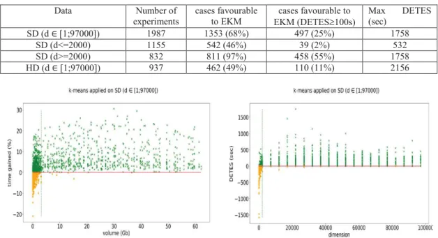
We evaluate, for spherical data and homogeneous data, the difference in execution time between the extended k-means version and the standard version. This difference will be called later in this document DETES. DETES is calculated as the difference between the time taken by the extended means and the standard k-means; it is positive when k-means extended is favourable compared to k-means standard, otherwise negative in the unfavourable case.

The Table 1. summarizes all the experiments performed on spherical and homogeneous data. The extended version shows better results in terms of execution time: out of 1987 experiments on spherical data (d& [1; 97000]), the extended version shows 1353 favourable cases (68%) where the DETES can reach 1758 seconds. We can also see that the performance of our extended version exceeds the standard version by more than 100 seconds in 25% of cases. The number of favourable cases is even more important when it comes to spherical data with dimensions d ³ 2000, since a favourable case rate of 97% is reached and with 55% having a DETES greater than 100 seconds.

Table 1: Favourable cases (%) to extended version k-means applied to SD and HD according to k (number of classes).

k SD ; d>=2000 HD; d>=2000 4 100% 67% 8 99% 71% 12 96% 68% 16 97% 66% 20 95% 55%

(6)

In Figures 1 to 4, we can observe the distribution of favourable and unfavourable cases. The horizontal (red) line separates favourable cases (green crosses) from unfavourable cases (orange circles) to extended k-means.

Figure 1 shows the percent of execution time gained by the extended version compared to the standard k-means: from 3.15 GB of data, the extended k-means is almost always favourable up to 30 % faster. In Figure 2, we can note that the extended version of k-means is clearly favourable from data of dimension greater than 2000 (green vertical line) where DETES reaches up to 1758 seconds (97% of favourable cases) whereas the average execution time of k-means standard is 3473 seconds. Unfavourable cases are mainly concentrated in the subspace of dimensions less than 2000.

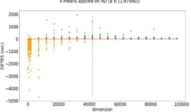
In Figures 3 and 4, we evaluate the behaviour of the both versions with homogeneous data. In Figure 3, the percentage of execution time gained by the extended version compared to standard k-means is approximately from 0 to 21% when the homogeneous data dimension is at least equivalent to 42000. As shown in Figure 4, the extended version is advantageous from 42000 dimensions. From this dimension, the average execution time of extended k-means is 1755 seconds. The gain can reach up to nearly 2156 seconds.

In the performed experiments, the influence of the parameter k (number of classes) was evaluated. We consider in Table 2 that the HD and SD datasets have dimension larger than 2000. The extended version unrolled on the spherical data gains with a very good rate clearly higher than 95% for classes ranging from 4 to 20. We can see that for k = 4 it gains 100%. Concerning homogeneous data, the favourable case rate is correct and is higher than 55% for classes 4 to 20. There is no decline or increase in favourable case rates as a function of k for either type of data distribution. The number of classes k does not alone influence the behaviour of the extended version of k-means. But favourable case rates in SD is largely favourable comparing to a distribution of HD data.

Table 2: Results of the executions of the both k-means versions on SD and HD.

Data Number of experiments cases favourable to EKM cases favourable to EKM (DETES³100s) Max DETES (sec) SD (d & [1;97000]) 1987 1353 (68%) 497 (25%) 1758 SD (d<=2000) 1155 542 (46%) 39 (2%) 532 SD (d>=2000) 832 811 (97%) 458 (55%) 1758 HD (d & [1;97000]) 937 462 (49%) 110 (11%) 2156

Figure 2: Evolution of the time differences (DETES) of the both versions of k-means according to the dimension. Figure 1: Time gained (%) by the EKM compared to the

(7)

Table 3: Percentage of centroids instances reused.

Figure 3: The time gained (%) by the EKM compared to the standard version as a function of the SD volume (GB).

Figure 4: Time gained (%) by the EKM compared to the standard version as a function of HD dimension.

Figure 5: DETES as a function of HD dimension.

4.3 The Proportions of the Reuse of the

Centroids According to the

Distribution HD and SD

The extended version does not obtain the same favourable case rate in both types of data distributions. It is more favourable on spherical data than on homogeneous data.

We consider two definitions of reuse of centroids. The first defines reuse as the number of reused centroids in a k-means execution. The second is the number of instances of centroids reused, i.e. if a centroid is reused p times it is said that there are p times reuses of the instance of this centroid.

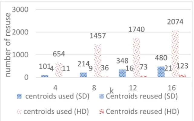
Table 3 and Figures 6-7 show results of experiment on reuse of centroids according to the data distribution (HD or SD), the number of classes k and the number of data points n (data size). Table 3 and figure 7 discuss the reuse of centroids instances while figure 6 discuss reuse of centroids without considering their instances. The experiment was performed under the same conditions as the previous one, but the dimension d is defined from 2 to 1802 with a step of 200, the size n&![20000 ;100000] with a step of 20000 and k&![4 ;16] with a step of 4.

In Figure 6, the number of centroids used SD is on average 6 times smaller compared to those in the case of HD. Similarly, the number of centroids reused among the centroids used remains marginal in SD and HD. It is practically 4% for each of the both distributions. Moreover, the more the number of classes k increases, the more the number of centroids used and reused also increases. This increase is more pronounced in HD.

In Figure 7, in each of the different k-means executions, the centroid whose instances were most reused was identified. The number of reuses of this centroid corresponds to "max reuse". Thus, "avg reuse" is the average of the number of the instances of all the centroids used in a k-means execution. "Max reuse" is about 2.5 times higher than the average reuse of the instances of the centroids (avg reuse) in the case of SD. It increases from two to nine times when k

k = 4 k = 8 k = 12 k = 16 Dataset size SD HD SD HD SD HD SD HD 20000 33% 5% 41% 15% 45% 19% 51% 27% 40000 32% 3% 44% 10% 50% 12% 55% 16% 60000 43% 3% 43% 7% 38% 12% 50% 19% 80000 40% 4% 53% 6% 50% 11% 53% 14% 100000 40% 3% 32% 4% 40% 7% 45% 12% AVG 37.6% 3.6% 42.6% 8.4% 44.6% 12.2% 50.8% 17.6%

(8)

increases in the case of HD. Moreover, when k increases "avg reuse" remains stable for both data distributions, it is approximately 2.5 and 18 respectively for DH and SD. This shows that the larger k is, the more the reuse of the centroids instances of a small set of centroids is increased but the stability of the average reuse of centroids instances is ensured when k increases.

Table 3 completes Figure 7. For each data distribution the proportion (%) of reused centroids instances is a function of the size of the data n and the number of classes k. This proportion is the average of the reused centroids for each dimension. The proportions of centroids reused in the extended version are superior in the case where it is applied on spherical data than in homogeneous data. For k = 4, the proportion is on average 37.6% for SD against 3.6% for HD that to say a difference of 30%. This difference is roughly similar for the other values of k, but the proportions in both distributions of data increase as k increases. In short, even if a subset of centroids is small compared to all of the centroids used through iterations in k-means, their instances are reused several times in order to exceed 50% of the reuses of centroids instances in the case of SD and 27% for HD. Also, experiments have shown that if a centroid is reused, it is reused successively over iterations. In other words, if the centroid is not reused in the iteration following the one where it was reused, it will no longer appear in all subsequent iterations.

4.4 Extended Gini Index

We found that our approach works better in spherical data than in homogeneous data. We used the gini index (Gini, 1921) to characterize a spherical dataset and predict in advance if our approach could be used. The gini index is a static measure used to measure the level of dispersion of a dataset.

%ABD E ,1 AFH + J + KDBMLN$ L J 1MLN$BL

(1)

% O,E {PQARSDTUV"W_{|X E K … Y}} (2)

EG = VAR(G*) (3)

Equation (1) defines G with S as a series of ordered positive numerical values. It is defined for univariate datasets. In our case, the data are multivariate. Let X be a dataset with d dimensions. The gini index is calculated for each dimension resulting in the list G* (equation 2). Finally, the variance of G* is calculated to obtain a scalar considered as the dispersion level of X (equation 3).

In practice, the cste constant of (equation 2) has been set to 10, which allows for a good separation of the two distributions.

In Figure 8, spherical datasets (green crosses) are distinguished from homogeneous data sets (orange circles). Each data set has a size between 20 000 and 100 000. There is a clear separation (horizontal line) between the both types of data according to the gini index EG. The limit is about EG =300.

Figure 6: Figures on reuse of centroids.

Figure 7: Figures on reuse of centroids instances.

Figure 8: Gini index EG as a function of dimension.

5 DISCUSSION

The extended k-means algorithm is advantageous on homogeneous data with numerous dimensions (if the

101 214 348 480 4 9 16 21 654 1457 1740 2074 11 36 73 123 0 1000 2000 3000 4 8 12 16 n u m b e r o f r e su se k

centroids used (SD) Centroids reused (SD)

centroids used (HD) Centroids reused (HD)

34 44 46 40 11 18 19 19 4 9 29 ₂₆ 2 2 3 3 0 10 20 30 40 50 4 8 12 16 n u m b e r o f r e u se k

Max reuse(SD) Avg reuse (SD)

(9)

dimension is at least equal to 42000) while it is advantageous on spherical data only from dimension 2000. In addition, the execution of both versions of k-means on spherical data is much faster than on homogeneous data. The k-means processes applied to homogeneous data calculate a significantly higher number of different centroids than those applied to spherical data if we consider that these processes adopt the same parameters (number of classes k, dimension d and size of data n). This difference therefore generates more iterations on homogeneous data than on spherical data and convergence is also slower. Among these different centroids, very few are used in k-means applied to homogeneous data. On the contrary, they are much reused in the case of k-means unrolled on spherical data, which explains why the extended k-means is much more favourable on these data than the homogeneous data.

If EKM is applied several times on the same dataset with different initializations of the centroids. It can be seen that the proportions of the reused centroids are not the same from one EKM execution to another. This observation is valid for both data distributions. So, the initialization of the centroids coupled with the choice of the distribution have an influence on our approach.

6 CONCLUSION

REFERENCES

Alsabti, K., Ranka, S. and Singh, V. (1997) ‘An efficient k-means clustering algorithm’, EECS

Arthur, D. and Vassilvitskii, S. (2007) ‘k-means++: the advantages of careful seeding’, SODA, pp. 1027–1025 Celebi, M. E., Kingravi, H. A. and Vela, P. A. (2013) ‘A

comparative study of efficient initialization methods for the k-means clustering algorithm’, ESA, pp. 200–210.

Deshpande, P. M. and al. (1998) ‘Caching

multidimensional queries using chunks’, in

Proceedings of the 1998 ACM SIGMOD, pp. 259–270.

Elkan, C. (2003) ‘Using the Triangle Inequality to Accelerate k-Means’, Proc.Twent. ICML, pp. 147–153. .

Forgy, E. W. (1965) ‘Cluster analysis of multivariate data: efficiency versus interpretability of classifications’,

Biometrics.

Gini, C. (1921) ‘Measurement of Inequality of Incomes’,

The Economic Journal. .

Gray, J. and al. (1996) ‘Data cube: A relational aggregation operator generalizing group-by, cross-tab, and sub-totals’, DMKD, 1(1), pp. 29–53.

Hamerly, G. (2010) ‘Making k -means even faster’, SDM

2010, pp. 130–140.

Hung, M.-C., Wu, J. and Chang, J.-H. (2005) ‘An Efficient

k-Means Clustering Algorithm Using Simple

Partitioning’, JISE 21, 1177, pp. 1157–1177.

Jain, A. K. (2010) ‘Data clustering: 50 years beyond K-means’, PRL. North-Holland, 31(8), pp. 651–666. Jain, A. K., Murty, M. N. and Flynn, P. J. (1999) ‘Data

clustering: a review’, CSUR, 31(3), pp. 264–323. Wasay, A. and al. (2017) ‘Data Canopy’, Proceedings of

the 2017 ACM SIGMOD ’17, pp. 557–572.

Zhang, J. and al. (2013) ‘A Parallel Clustering Algorithm with MPI – MKmeans’, JCP, 8(1), pp. 10–17. Zhao, Weizhong; Ma, Huifang; He, Q. (2009) ‘Parallel K

-Means Clustering Based on MapReduce’, CLOUD Zhao, W. L., Deng, C. H. and Ngo, C. W. (2018) ‘k-means:

A revisit’, Neurocomputing, 291, pp. 195–206.

In this paper, we provided an approach to accelerate the process of the unsupervised data learning algorithm, called k-means. This approach is based on an algorithm that pre-calculates and stores intermediate results, called dynamic pre-aggregates, to be reused in subsequent iterations. Our experiments compare our extended k-means version with the standard version using two types of data (spherical and homogeneous data). 2798 synthetic datasets that have been generated reaching up to 62GB. We demonstrate that our approach is advantageous for partitioning large datasets from dimensions 2000 and 42000 respectively for spherical data and homogeneous data.

Several perspectives are planned. We are ongoing to experiment our extended version of k-means with even more massive data to better evaluate the cost of calculating pre-aggregates. In addition, it is proposed to study situations where it might be more effective to start from an archived centroid corresponding to a class almost similar to the new class encountered rather than recalculate it entirely on the pretext that the class is not exactly identical.