ESSAYS IN MACROECONO:NIICS ON SHORT-TERM
DYNAMICS OF INFLATION AND FINANCIAL MARKETS
THESIS
PRESENTED
AS PARTIAL REQUIRElV
IENT
OF DOCTORAL OF PHILOSOPHY IN
ECONOMICS
BY
YOROU TCHAKONDO
Avertissement
La diffusion de cette thèse se fait dans le respect des droits de son auteur, qui a signé le formulaire Autorisation de reproduire et de diffuser un travail de recherche de cycles supérieurs (SDU-522 - Rév.0?-201 1 ). Cette autorisation stipule que «conformément à l'article 1 1 du Règlement no 8 des études de cycles supérieurs, [l'auteur] concède à l'Université du Québec à Montréal une licence non exclusive d'utilisation et de publication de la totalité ou d'une partie importante de [son] travail de recherche pour des fins pédagogiques et non commerciales. Plus précisément, [l'auteur] autorise l'Université du Québec à Montréal à reproduire, diffuser, prêter, distribuer ou vendre des copies de [son] travail de recherche à des fins non commerciales sur quelque support que ce soit, y compris l'Internet. Cette licence et cette autorisation n'entraînent pas une renonciation de [la] part [de l'auteur] à [ses] droits moraux ni à [ses] droits de propriété intellectuelle. Sauf entente contraire, [l'auteur] conserve la liberté de diffuser et de commercialiser ou non ce travail dont [il] possède un exemplaire.»
ESSAIS EN MACROÉCONONIIE SUR LES DYNAMIQUES
À
COURT TERME DE L
'INFLATION ET LES
MARCHÉS
FINANCIERS
THÈSE
PRÉSENTÉE
COMNIE EXIGENCE PARTIELLE
DU DOCTORAT EN ÉCONOMIQUE
PAR
YOROU TCHAKONDO
Je voudrais exprimer toute ma gratitude à mes directeurs de recherche, Louis Phaneuf et Alessandro Barattieri pour leur direction, leur aide et leur sou-tien financier et moral dans la réalisation de cette thèse. Sans mes directeurs de recherche, ce travail n'aurait jamais été possible. 'Ifavailler sous leur direction a été une expérience scientifique formidable et une véritable école de la vie. Qu'ils reçoivent en quelques lignes ici mes sincères remerciements. Mes remerciements aussi aux professeurs et membres du jury Julien Martin, Christian Sigouin et Dali-bor Stevanovic pour leurs remarques et commentaires pertinents qui m'ont permis de bonifier cette thèse.
Mes remerciements à Steven Ambler, Pavel Sevcik, et Pierre-Yves Yanni du département des sciences économiques de l'UQAI\.1 pour leurs commentaires judicieux dont a bénéficié cette thèse. Je suis également reconnaissant aux autres enseignants du département, notamment Max Blouin, Alain Delacroix, Claude Felteau, Claude Fluet, Jean-Denis Garon, Alain Guay, Douglas Hodgson, Wilfried Koch, Philip :tvlerrigan, Victoria Miller et Alain Paquet pour tout ce qu'ils m'ont apporté.
Je voudrais aussi témoigner ma reconnaissance à Martine Boisselle, Lorraine Brisson, Hélène Diatta, Francine Germain, Julie Hudon, Jacinthe Lalonde et Josée Parenteau du personnel administratif du département pour leur aide, patience et disponibilité.
L'accomplissement de cette thèse a également été possibe grâce aux conseils, recommandations, encouragements et apports d'autres enseignants. Ainsi, à PUQAM, j adresse mes remerciements à Charles Langford, Komlan Sedzro et Pater Twara-bimenye du département de Finance, Nicole Lanoue du département des sciences comptables, Lassana Maguiraga du département de management et technologie, Abdellatif Obaid du département d'informatique et Sorana Froda du département de mathématiques. Ma reconnaissance également à Marc Henry du département d'économie à PennState University, Jean-Niarie Dufour et Francisco Ruge-Murcia du département d'économie de McGill University, Silvia Goncalves et William Mccausland du département d économie de l'Université de Montréal.
Pendant la période de ma thèse, j'ai eu la chance de rencontrer, d'échanger et de communiquer avec beaucoup d'amis, aussi bien de l'UQAM que d'autres univer-sités. J'aimerais tous les remercier pour tout ce qu'ils ont fait pour moi. Je citerai
Carvajalino, Afef Chouchane Ismael Crèvecœur, Carla Cruz, Rose Dabire, Bouba-car DiaJlo, Antoine Djogbenou, Koffi Elitcha, vVilliam Ewane, William Gbohoui, Sylvain Guay, Bouba Housseini, Jonathan Lachaine, François Laliberté, Thomas Lalime, Mouna Landolsi, Martin Leblond, William Leroux, Adil Mahroug, Hami-dou Mbaye, Alexis Manette, Ismael Momifie, Oualid Moussouni, Kelly N'dri, Thu Nguyen, Idrissa Ouili, Dang Pham, Aliou Sa.ll, Jean-Blaise Nlefu, Aligui Tientao, Abder El Trach, Jean-Paul Tsa.c;a, Vincent Tsoungui, Benoit Vincent, Jean-Gardy Victor, Joris Wauters, Hamidou Zanré, Karnel Zeghba et Hervé Zongo.
Je ne saurais jamais assez remercier l'ensemble de ma famille pour l'immense influence qu'elle a eue sur la réalisation de cette thèse. D'abord, mes parents, T cha-kondo Banavèye et Sibabé Alia pour m'avoir donné la vie, aimé, élevé, éduqué et envoyé à l'école. Que mon épouse Charlotte Tkaczyk reçoive ici toute ma pro-fonde gratitude pour son amour, sa patience, sa compréhension et le soutien sans faille qu'elle m a apporté durant toute cette période. Je remercie infiniment notre fille Suzanne Solim Tchakondo pour le bonheur, la joie et le courage qu'elle m 'in-suffie depuis qu'elle est parmi nous. Je voudrais également dire un grand merci à mes beaux-parents, Catherine et Jean-Luc Tkaczyk pour le soutien qu'ils m'ont témoigné, sans oublier Babtchia, Edmond, Mamie, athalie, Séverine, Sophie et Vincent. Merci aussi au reste de ma famille au Togo notamment, Abass, Aicha Alasa, Alimotou, Amidou, Anoko Aridja, Bamoi, Bitou, Derman, Fali, Gado Kerim, Nasser, Nima, Raouf, Safoura, Saibou, Sourouma, Taffa et Zakari.
Je dédie par ailleurs cette thèse à mes amis Achille Abotsi, Maurice Ada-rnou, Denis Agba, Grégoire Agba, Mashoudi Agbagni, Nawel Akacem, Géneviève Akotia, Akilou Amadou, Koffi Anoumou, Safiou Ayeva, Yannick Bigah, Gabriela Carmona, Razak Cissé, Azimaré Djobo, Mamadou Dramé, Gaffo Ezoula, Lati-fou Ezoula, Razak Fabulous, Prosper Gaglo, Kodjo Gbenyo, Ben Guinhouya, Moussoulim Issa-Touré, Rouf ai Issifou, Y amin ou Issifou, Edgard Kabaguntsi, Iki-lilou Kerim, Jean Kima, Elom Komlan, Aboubacar Kondoou, Kangni Kpodar, Jolly Aloessodé, Taffa Mamadou, Franco Napo-Koura, Michael Olornadjehé, Awali Ouro-Koura, Jérémie Modjinou, Lamine Sambou, Essognina Sidibé, Eli Sodoké, Didier Tagbata, Abou Taulier, Bassarou Tchagodomou, Meriga Tchagodomou, Tagba Tchagouni, Ibrahim Tchakala, Sani Tchakondo, Sourak Tchanilé, Nasser Tchassanti, Ali Tchatchassé, Assoumanou Tir et Aziz Zakari.
Je ne saurais finir ces remerciements sans avoir une pensée pour mes ensei-gnants aux primaire, collège, lycée et université au Togo en particulier, Akoussah, Akpaka, Bakatra, Directrice, Esso, Gadégbé et Kouloba pour m'avoir mis le pied à l'étrier.
LIST OF FIGURES vm LIST OF TABLES x RÉSU:tviÉ 0 0 Xl ABSTRACT Xlll INTRODUCTION 1 CHAPTER I
THE NE'vV KEY ESIAN PHILLIPS CURVE: INTERMEDIATE GOODS
MEET POSITIVE TRE D I IFLATIO 5
1.1 Introduction 0 0 0 0 0 0 0 0 0 0 0 6
1.2 The Varions Incarnations of the KPC 0 1.201 The Forward-Looking NKPC 0 0
1.202 Backward-Looking Elements and the KPC 1.203 Trend Inflation and the NKPC 0 0 0
10 11 12 13 1.3 A NKPC Model with Intermediate Goods and Positive Trend Inflation 14
1.301 Optimal Pricing Decisions 1.302 Monetary Policy 0 0 0 0 0
1.303 Equilibrium and Market-Clearing Conditions 0
15 18 18 1.4 The NKPC: Intermediate Goods Meet Positive 1\·end Inflabon 0 19
1.4.1 Optimal Pricing Decisions with Intermediate Goods and Non-Zero Trend Inflation 0 0 0 0 0 0 0 0 0 0 0 0 0 0 0 0 0 0 0 0 0 0 0 19 1.402 The KPC with Intermediate Goods and on-Zero 1\·end
In-flation 0 0 0 0 0 0 1.5 Calibration and Results 0 0 0
1.501 Calibrated Parameters
1.502 The NKPC: Intermediate Goods vs Trend Inflation
21 22 22 24
1.6 Conclusion . 27 CHAPTER II
INFLATION PERSISTENCE IN DSGE MO DELS: A EMPIRICAL
ANAL-YSIS . . . . . . . 31
2.1 Introduction . . . . . 32
2.2 The Model Economy 35
2.2.1 Households 2.2.2 Firms . . . 2.2.3 Monetary Policy
2.2.4 Equilibrium and Market-Clearing Conditions .
35 37 41 41 2.3 Calibration 42 2.4 Results . . . 45 2.5 Conclusion . 49 CHAPTER III
FI ANCIAL MARKETS AND THE CAPITAL ASSET PRICI G MO DEL
IN A DSGE FRAMEWORK 60
3.1 Introduction . . . . 61
3.2 The Model Economy.
3.2.1 Firms: Optimal priee setting.
3.2.2 Households: Portfolio choice decisions 3.2.3 Financial markets: The CAPM 3.2.4 Central bank . . . . . . . . 3.2.5 Markets clearing conditions 3.3 Calibration
3.4 Results . . .
3.4.1 Responses to technology shock 3.4.2 Responses to monetary policy shock 3.4.3 Responses to financial market shock
65 65 67
70
74 74 75 77 77 78 783.4.4 Volatilities and autocorrelations . 81
3.5 Conclusion . 83
CONCLUffiON . ~
APPENDIX A
FI ANCIAL MARKETS AND THE CAPITAL ASSET PRICI G MO DEL IN A DSGE FRAMEWORK . . . . . . . . . . . . . . . . . . . . . . . . . 95
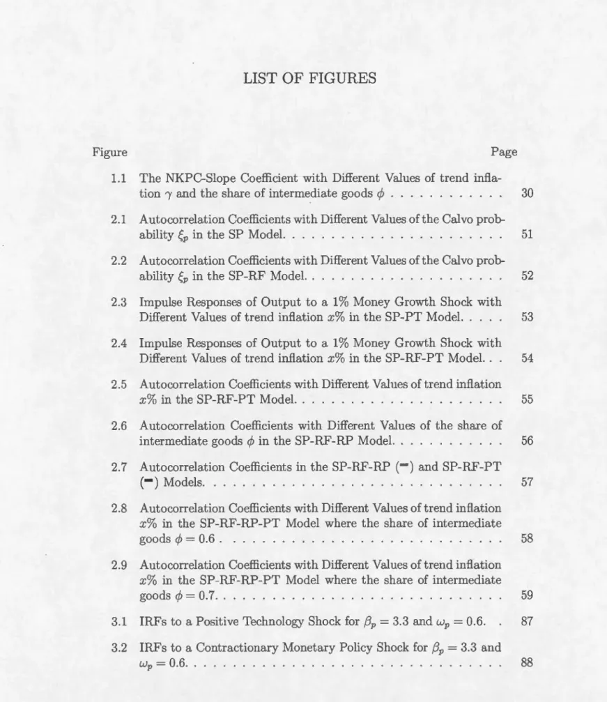
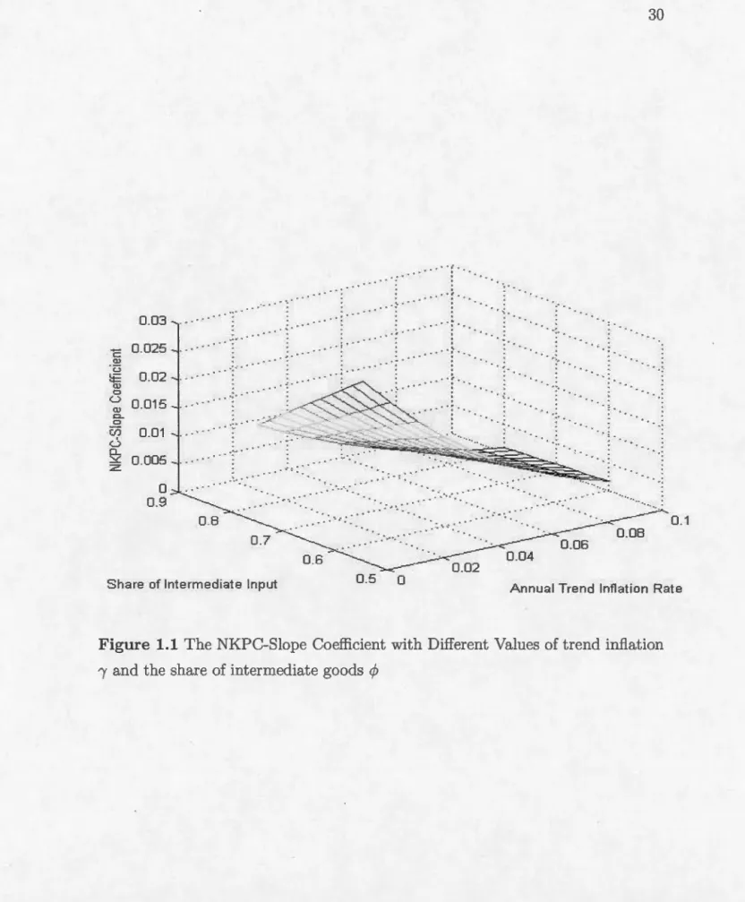
Figure Page 1.1 The NKPC-Slope Coefficient with Different Values of trend infl
a-tion 1 and the share of intermediate goods
cp
.
.
.
.
.
.
.
.
.
.
.
.
30 2.1 Autocorrelation Coefficients with Different Values of the Calvoprob-ability Çp in the SP Model. . . . . . . . . . . . . . . . . . . . 51 2.2 Autocorrelation Coefficients with Different Values of the Calvo
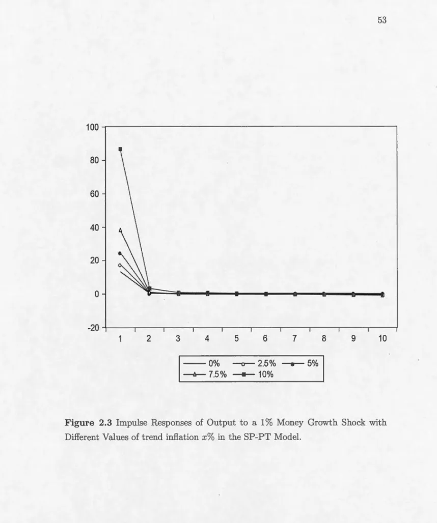
prob-ability Çp in the SP-RF Model. . . . . . . . . . . . . . 52 2.3 Impulse Responses of Output to a 1% Money Growth Shock with
Different Values of trend inflation
x%
in the SP-PT Model. . . . . 53 2.4 Impulse Responses of Output to a 1% :t-.1oney Growth Shock withDifferent Values of trend inflation
x%
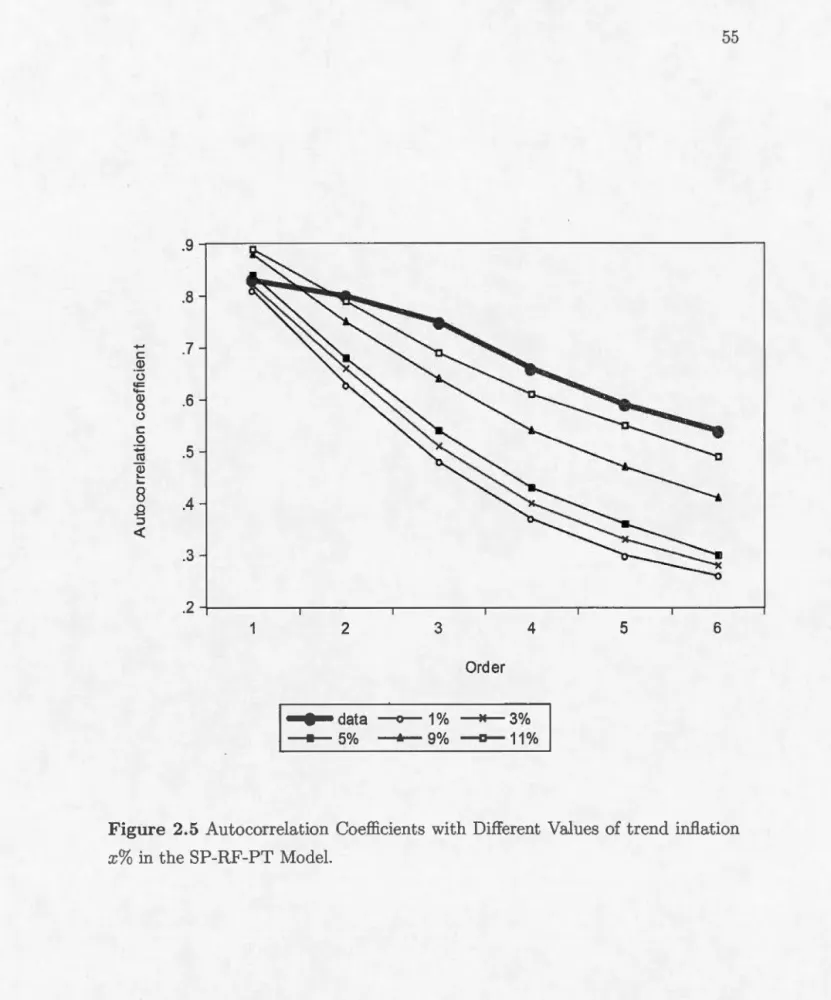
in the SP-RF-PT Model. . . 54 2.5 Autocorrelation Coefficients with Different Values of trend inflationx%
in the SP-RF-PT Model. . . . . . . . . . . . . . . . . . 55 2.6 Autocorrelation Coefficients with Different Values of the share ofintermediate goods
cp
in the SP-RF-RP Model. . . . . . . . . 56 2.7 Autocorrelation Coefficients in the SP-RF-RP (- ) and SP-RF-PT(- ) Models. . . . . . . . . . . . . . . . . . . . . . . . . . . . . 57 2.8 Autocorrelation Coefficients with Different Values of trend inflation
x%
in the SP-RF-RP-PT Model where the share of intermediate goodscp
=
0.6 . . . . . . . . . . . . . . . . . . . . . . . . 58 2.9 Autocorrelation Coefficients with Different Values of trend inflationx%
in the SP-RF-RP-PT Model where the share of intermediate goodscp
=
0.7. . . . . . . . . . . . . . . . . . . . . . . . . . . 59 3.1 IRFs to a Positive Technology Shock for {Jp = 3.3 and wP= 0.6
. 87 3.2 IRFs to a Contractionary Monetary Policy Shock for {Jp = 3.3 and303 IRFs to a Positive Financial Market Shock for {3p > 1 and wp = 006 0 89 304 IRFs to a Positive Financial Market Shock for {3p
=
303, {3p=
505and wP = 0060 0 0 0 0 0 0 0 0 0 0 0 0 0 0 0 0 0 0 0 0 0 0 0 0 0 0 0 0 0 90
305 IRFs to a Positive Financial Market Shock for wP
=
006, wP=
004 and {3p = 3030 0 0 0 0 0 0 0 0 0 0 0 0 0 0 0 0 0 0 0 0 0 0 0 0 0 0 0 0 0 91 306 IRFs to a Positive Financial Market Shock for {3P < 0 and wP = 0060 92LIST
OF TABLES
Tableau Page
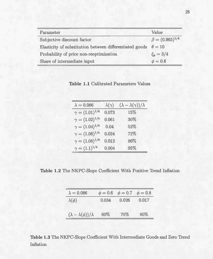
1.1 Calibrated Para.meters Values 28
1.2 The NKPC-Slope Coefficient With Positive Trend Inflation 28
1.3 The NKPC-Slope Coefficient With Intermediate Goods and Zero Trend Inflation . . . . . . . . . . . . . . . . 28 1.4 The NKPC-Slope Coefficient With Intermediate Goods and
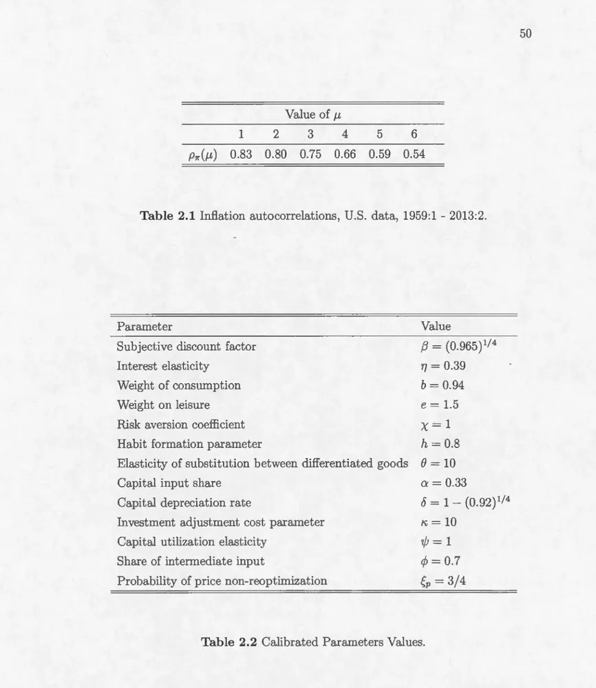
Posi-tive Trend Inflation . . . . . . . . . . . . 29 2.1 Inflation autocorrelations, U.S. data, 1959:1 - 2013:2. 50
2.2 Calibrated Parameters Values. 50
3.1 Calibrated Parameters Values 84
3.2 Standard Deviations and Relative Volatilities (Data: 1954Q1-2008Q3) 85
Cette thèse comprend trois chapitres relatifs aux dynamiques à court terme de l'inflation et à l'impact des marchés financiers sur l'économie réelle.
Le premier chapitre propose un modèle d'équilibre général dynamique et stochastique (DSG E) qui incorpore une structure en boucle de production à côté du trend d'inflation positif, afin d'analyser les sources des dynamiques à court terme de l'inflation. Il s'agit principalement de développer pour la première fois dans la littérature et en présence de ces deux ingrédients, une formulation générale de la courbe de Phillips néo-keynésienne où, l'inflation est exprimée comme une fonction des coûts marginaux réels et de l'inflation future anticipée. En se concen-trant sur l'analyse de la pente de la courbe de Phillips, nous montrons que le trend d'inflation positif et la structure en boucle de production sont nécessaires pour expliquer la persistance de 1 'inflation observée dans les données. Cependant, sous des valeurs raisonnables du trend d'inflation, les inputs intermédiaires jouent un rôle beaucoup plus important que le trend d'inflation en ce qui concerne la persistance inflationniste.
Dans le deuxième chapitre, nous visons à approfondir notre compréhension des dynamiques à court terme de l'inflation. Pour ce faire, nous simulons un modèle DSGE qui intègre non seulement la structure en boucle de production et le trend d'inflation positif, mais aussi des frictions réelles comme la formation d'habitude de consommation, les coûts d'ajustement du capital et l'utilisation variable du ca-pital. Les autocorrélations théoriques de l'inflation obtenues du modèle simulé sont ensuite confrontées à celles observées dans les données de 1 économie américaine. Les conclusions de la démarche analytique du premier chapitre sont confirmées ici. En effet, nous trouvons d'une part que le trend d'inflation positif a un effet négligeable sur la persistance de l'inflation en présence des inputs intermédiaires. D'autre part, la structure en boucle de production fournit une meilleure explica-tion de l'évidence empirique sur la persistance de l'inflation.
Le troisième chapitre étudie les interconnections entre les marchés financiers et l'économie réelle. Le cadre d'analyse est un modèle DSGE qui rend compte des interventions des ménages sur les marchés financiers, à travers le modèle d'évaluation des actifs financiers de Fama et French (2004). Par ailleurs, nous proposons une modélisation explicite des dynan1iques des marchés financiers sur
la base du mouvement brownien géométrique. Comme résultats, nous montrons que la consommation, l'output et l'investissement réagissent moins alors que l'in-flation et le travail réagissent plus fortement au choc technologique ici, que dans le cas d'une économie où le secteur financier est ignoré. En outre, les effets négatifs d'un choc de politique monétaire restrictive sur l'output, la consmrunation, l'in-flation, l'investissement et le travail sont beaucoup plus importants. Par ailleurs, nous trouvons qu'un choc positif aux marchés financiers exerce une pression à la baisse sur le taux œintérêt nominal lorsque le coefficient beta du portefeuille d'actifs du ménage est positif. Enfin, le modèle DSGE avec le secteur financier reproduit mieux la plupart des caractéristiques de l'économe U.S., en particulier, les volatilités et autocorrélations des principales variables macroéconomiques ainsi que leurs corrélations avec l'output.
Mots-clés : Dynamiques de 1 inflation, persistance de l'inflation, prix ri-gides, biens intermédiaires, trend d'inflation positif, production en boucle, CAPM, marchés boursiers, politique monétaire, choix de portefeuille, mouvement brow -nien géométrique.
This thesis consists of three chapters related to short-term dynamics of inflation and the impact of financial markets on the real economy.
The first chapter offers a dynamic stochastic general equilibrium (DSGE) model that incorporates a roundabout structure of production alongside a positive inflation trend, to analyze the sources of short-term dynamics of inflation. In presence of both ingredients, the main goal here is to develop for the first time in the literature, a general New Keynesiru1 Phillips Curve (NKPC) formulation, where inflation is expressed as a function of real marginal costs and expected future inflation. Focusing in our ru1alysis on the NKPC-slope coefficient, we show that both ingredients are necessary to account for inflation persistence observed in the data. However, under plausible values of trend inflation, intermediate goods play a more significant role shaping inflation persistence thru1 trend inflation.
In the second chapter, we aim to deepen our understanding of short-term dynamics of inflation. To do so, we simulate a DSGE model that incorporates not only roundabout production and positive trend inflation, but also real frictions such as habit formation, capital adjustment costs and variable capital utilization. The theoretical autocorrelations of inflation obtained from the simulated model are then compared with those observed in the U.S. data. The findings of the analytical approach of the first chapter are confirmed here. In fact, we find first that the positive trend inflation appears to have a negligible impact on inflation persistence when allowing for roundabout production. Second, intermediate goods provide a better explru1ation of the empirical evidence on inflation persistence.
The third chapter explores the interconnections between financial markets and the real economy. The framework is a DSGE model that accounts for house-holds interventions on financial markets, through the capital asset pricing model (CAPM) of Fama and French (2004). Moreover, we propose an explicit modelling of financial markets dynamics based on geometrie brownian motion. As results, we show that consumption, output and investment react less to a technology shock, while the nominal interest rate, inflation and labor are responding more strongly, compared to the case where financial markets are ignored. Moreover, the negative effects of a tightening monetary policy shock on output, consumption, inflation, investment and labor are more significant. Vve also find that a positive
financial markets shock exerts a downward pressure on the nominal interest rate when the beta coefficient of the assets portfolio is positive. Finally, we find that our model with a financial market sector is successful in reproducing most of the salient features of the U .S. economy, particularly, key macroeconomie volatilities, autocorrelations, and correlations with output.
Keywords: Inflation dynamics, inflation persistence, sticky priees, inter-mediate goods, positive trend inflation, roundabout production, CAPî-.ii, stock markets, monetary policy, portfolio choice, geometrie brownian motion.
Le principal défi auquel s'attaque notre thèse est d aider non seulement à une meilleure mise en application de la politique monétaire, mais aussi, à un examen beaucoup plus approfondi des effets de cette dernière sur l'économie réelle. Cela passe par deux canaux de recherche. D'abord, un objectif de maîtrise des dynamiques à court terme de l'inflation par les banques centrales et les chercheurs, ce à quoi s'attèlent les deux premiers chapitres. Puis, une grande compréhension
par la communauté scientifique de l'analyse des interconnections entre les marchés
financiers et l'économie réelle que constitue l'objet du dernier chapitre.
Une relation structurelle clé dans la catégorie des modèles d'équilibre général dynamique et stochastique (DSGE) est la courbe de Phillips néo-keynésienne (NKPC). La NKPC a connu ces dernières années, plusieurs développements visant à mieux expliquer les dynamiques à court terme de 1 'inflation et à améliorer de manière générale notre compréhension de la politique monétaire. La NKPC stan-dard est log-linéarisée autour d'un trend d'inflation nul. Cette hypothèse est d'une part, contrefactuelle à cause d'un taux d'inflation en moyenne positif enregistré par les économies industrialisées de l'après-guerre, et d'autre part, non anodine comme tente de démontrer un courant de littérature récent. Ascru·i (2004) par exemple, montre que le trend d'inflation positif pourrait affecter de manière signi-ficative les propriétés de court terme et de long terme des modèles à prix rigides, alors que Ascari et Ropele (2007) et Coibion et Gorodnichenko (2011) trouvent que même un trend d'inflation faible aurait un impact sur la politique monétaire optimale et les dynamiques des variables macroéconomiques.
Cette thèse explore entre autres, et ce, à travers les deux premiers chapitres, la NKPC et les sources des dynamiques de l'inflation dans une économie avec trend d'inflation positif. Mais pour la première fois dans ce type de littérature,
-nous traitons cette problématique en utilisant un modèle DSGE qui incorpore non seulement le trend d'inflation positif, mais aussi et surtout une structure en boucle de production. La prise en compte de la structure en boucle de production est motivée par le fait que les biens finaux sont devenus de plus en plus sophistiqués et complexes en termes de production, notamment de la période de l'entre-deux guerres à la période de l'après-guerre (voir, Basu et Taylor, 1999a, 1999b; Ranes, 1996, 1999; Huang, Liu et Phaneuf, 2004). Au début du dix-neuvième siècle, le panier de consommation du ménage était principalement composé de biens rela-tivement non finis. Depuis lors, les économies industrialisées ont été caractérisées par une augmentation des relations inputs-outputs dans la production des types de biens entrant dans le panier de consommation finale. Huang, Liu et Phaneuf (2004) montrent que la part U.S. des inputs intermédiaires a augmenté de 0.3 - 0.4 durant la période de l'entre-deux guerres à 0.6 - 0.7 durant la période de l'après-guerre, tandis que diverses études estiment que cette part se situe entre 0.6 et 0.9 pour la période de l'après-guerre (voir, Basu, 1995; Bergin et Feenstra, 2000; Huang et Liu, 2001; Huang, Liu et Phaneuf, 2004; Naka.mura et Steinsson, 2010).
Ainsi, le premier chapitre propose pour la première fois dans ce type de modèles DSGE, et en présence de la boucle de producton et du trend positif, une formulation générale de la KPC où l'inflation est exprimée comme une fonction des coüts marginaux réels et de l'inflation future anticipée. Nous trouvons ici que les interactions entre les prix rigides, les inputs intermédiaires et le trend d'inflation positif ont une forte influence sur la sensibilité de l'inflation aux coüts marginaux réels. Toutefois, les biens intermédiaires semblent avoir un impact plus important sur le coefficient de la pente de la KPC que le trend d'inflation positif suggéré par Ascari ( 2004).
Dans le même ordre d'idées, le deuxième chapitre est une extension du modèle DSGE à trend d'inflation positif de Ascari (2004). Nous bonifions ce modèle en intégrant non seulement la structure en boucle de production, mais aussi diverses frictions réelles comme la formation d'habitude de consommation, les coûts d'ajustement du capital et l'utilisation variable du capitaL Ces
fric-tions réelles standard dans la littérature DSGE, semblent incontournables dès lors qu'on veut analyser la persistance des variables macroéconomiques (CEE, 2005; Smets and vVouters, 2003). La démarche ici, consiste d'abord à générer les autocorrélations de l'inflation à partir du modèle simulé, et ensuite, à les comparer à celles observées dans les données de 1 économie américaine. Il s'en suit que le trend d'inflation positif a un effet négligeable sur les dynamiques de l'inflation en présence des inputs intermédiaires, et que ces derniers donnent une meilleure explication de l'évidence empirique sur la persistance de l'inflation. Ces résultats confortent ainsi nos conclusions de la démarche analytique du premier chapitre.
Enfin le troisième chapitre s'inscrit dans la deuxième problématique de notre thèse, à savoir, les interconnections entres les marchés financiers et l'économie réelle. Le point de départ de ce travail est la récente crise financière de 2008, qui a montré comment des chocs négatifs aux marchés financiers pouvaient se transformer en des conséquences néfastes pour l'économie réelle. Cette crise a aussi mis en évidence l'inefficacité des instruments traditionnels de la politique monétaire dans un contexte de taux d'intérêt proches de la borne zéro. D'oü, la nécessité d'un plus grand intérêt pour les marchés financiers ainsi qu'une anal-yse plus poussée de leurs impacts sur l'économie réelle. Nous nous attelons à cela en proposant un cadre d'analyse DSGE qui intègre le modèle d'évaluation des actifs financiers, pour rendre compte des interventions des ménages sur les marchés financiers (voir, Markm;<,ritz, 1959; Sharpe, 1964; Lintner, 1965; Fama, 1996; et Fama et French, 2004). Le modèle d'évaluation des actifs financiers sup-pose que les individus détiennent un portefeuille d'actifs composé d'actifs sans risque, et d'actifs risqués disponibles sur les marchés boursiers. De plus, une modélisation explicite des dynamiques des marchés financiers est proposée en se basant sur le mouvement brownien géométrique (voir, Kendall et Hill, 1953; Os-borne, 1959; Roberts, 1959; Samuelson, 1965; Black et Scholes, 1973; Barmish et Primbs, 2011; et Lochowski et Thagunna, 2013). Nos résultats suggèrent que la consommation, l'output et l'investissement réagissent moins, alors que l'inflation et le travail réagissent plus fortement au choc technologique ici, que dans le cas d'une économie oü le secteur financier est ignoré. Aussi, les effets négatifs d'un
choc de politique monétaire restrictive sur l'output, la consommation, l'inflation, l'investissement et le travail sont beaucoup plus importants. Par ailleurs, nous trouvons qu'un choc positif aux marchés financiers exerce une pression à la baisse sur le taux d'intérêt nominal lorsque le coefficient beta du portefeuille d'actifs du ménage est positif. Enfin, le modèle DSGE avec le secteur financier repro-duit mieux la plupart des caractéristiques de l'économe U.S., en particulier, les volatilités et autocorrélations des principales variables macroéconomiques ainsi que leurs corrélations avec l'output. Par conséquent, les marchés financiers, et plus précisément les marchés boursiers mériteraient une attention particulière de la part des autorités monétaires et des chercheurs, lorsqu'on vise à mieux com-prendre les tenants et aboutissants de la politique monétaire.
THE NEW KEYNESIAN PHILLIPS CURVE: INTERMEDIATE
GOODS
MEET
POSITIVE
TREND
INFLATION
Abstract
What happens when intermediate goods meet positive trend inflation in a ew Keynesian Phillips Cmve (NKPC) madel? Focusing on the slope coefficient on marginal cost, our analysis shows the effects are dramatic. Unlike the basic Calvo price-setting madel which requires an extremely law frequency of priee adjustment or backward-looking components to account for inflation persistence, om madel with sticky priees, roundabout production and trend inflation does successfully so with a plausible fre-quency of priee changes, and realistic values of trend inflation and share of intermediate inputs. While trend inflation plays a non negligible role in explaining inflation dynamics,
accounting for roundabout production seems to be more important.
JEL classification: E31, E32.
1
.
1
Introduction
A key structural relationship in a large class of dynamic stochastic gen-eral equilibrium (DSGE) models is the so-callcd New Keynesian Phillips curve ( KPC). The NKPC has undergone sever al developments in recent years aimed at better tracking short-run inflation dynamics and improving our understanding of monetary policy more generally. The standard NKPC is log-linearizcd around a zero steady-state rate of inflation. This assumption is not only counterfactual since postwar industrialized economies have experienced positive inflation on aver-age, it is not innocuous as a recent body of research tends to demonstrate. Ascari (2004), for instance, shows that positive trend inflation may significantly alter the short-run and long-run properties of sticky-price models, while Ascari and Ropele (2007) and Coibion and Gorodnichenko (2011) argue that even low trend inflation may affect optimal monetary policy and the dynamics of macro variables.
The present paper further explores the KPC and the sources of inflation dynamics in an economy with positive trend inflation. But for the first time in this type of literature, wc address this question using a DSGE framework in which intermediate goods meet positive trend inflation. Focusing in our analysis on the dynamic response of inflation to real marginal costs (Galf and Gertler,
1999; Ascari 2004), to which we refer throughout the paper as slope coefficient
on marginal cast or NKPC-slope coefficient, we show that both ingredients are
necessary to account for the observed inertial behavior of inflation, but that under plausible values of trend inflation, intermediate goods play a more significant role shaping inflation dynamics than trend inflation.
A well known property of the basic new keynesian sticky-price model with zero trend inflation is that the NKPC is purely forward-looking in that current inflation depends on current real marginal costs and expected future inflation. As we discuss in Section 2 of the paper, the basic KPC is hardly reconcilable with the inertial behavior of inflation unless assuming an implausibly long aver-age waiting time between priee adjustments, backward-looking components (Gal! and Gertler, 1999; Christiano, Eichenbaum and Evans, 2005; Smets and Vlouters,
2007; Justiniano and Primiceri, 2008), or slow-moving (random walk) trend infla
-tion (Cogley and Sbordone, 2008).
Here, we combine a roundabout production structure with non-zero steady -state inflation in Calvo's (1983) price-setting framework. Previous research has established that in arder to generate a high positive serial correlation of inflation as observed in the U.S. data, the basic KPC requires assuming a very high prob -ability of priee non-reoptimization. Vlorking from the Calvo sticky-price madel of King and ·watson (1996), Nelson (1998, Table 3) shows that this probability must be close to 0.9 to match inflation persistence. This in turn implies an average waiting time between priee adjustments of 2.5 years or more, which clearly is c oun-terfactual. With a subjective discount factor of 0.99, the NKPC-slope coefficient would have to be 0.012 more or less. If the probability of priee non-reoptimization is set instead at the more conventional value of O. 75, the NKPC-slope coefficient increases to 0.086, which is 7 times larger than required to match inflation inertia. The inability of the basic NKPC model to account for inflation persistence without assuming an implausibly low frequency of priee adjustments has led re
-searchers to incorporate mechanisms like rule-of-thumb behavior of priee-setters, backward indexation of priees, and slow-moving trend inflation in new keynesian pricing models (Galf and Gertler, 1999; Christiano, Eichenbaum and Evans, 2005;
Smets and ~Touters, 2007; Justiniano and Primiceri, 2008; Cogley and Sbordone, 2008).
Contrasting sharply with previous studies, our approach does not need to rely on such ingredients to be consistent with inflation persistence. Still, it is fully. consistent with the optimizing behavior of households and firms. Our framework is one that exploits strong interactions between a roundabout production structure, sticky priees and positive trend inflation. Our use of a roundabout production structure is motivated by the fact that final goods have become more processed and increasingly sophisticated over time, especially from the interwar period to the postwar period (e.g., Basu and Taylor, 1999a, 1999b; Ranes, 1996, 1999; Huang,
ump-tion basket was primarily composed of relatively unfinished goods. Since then,
industrialized economies have been characterized by increased roundaboutness in the production of typical goods entering the final consumption basket. 1 Huang,
Liu and Phaneuf (2004) document that the U.S. share of intermediate inputs has
risen from 0.3- 0.4 during the interwar period to 0.6- 0.7 during the postwar period, _wherea..s a variety of studies evaluate that this share lies between 0.6 and
0.9 for the postwar period. 2
Working from a state-dependent model with nominal priee rigidity, Basu
(1995) shows that eombining input-output linkages between firms with small (menu) eost of ehanging priees ean give rise to a multiplier for priee stiekiness (IviPS): beeause all firms in the eeonomy face sticky priees and use intermediate
inputs, firms' prieing decisions beeome intereonneeted, so that the an1ount of priee stiekiness at the aggregate level may well exceed that observed at the individual firm level. Using a fully artieulated DSGE model with nominal and real frictions,
El Omari and Phaneuf (2011) provide quantitative evidence that the MPS may
be an important source of inflation inertia and persistenee in aggregate quantities
in a Calvo wage-and-price-setting framework with zero steady-state inflation. Aseari (2004) extends the standard new keynesian prieing model to aeeount
for positive trend inflation, showing that positive steady-state inflation ean s ig-nifieantly flatten the NKPC while redueing the sensitivity of eurrent inflation to
the eurrent output gap. For example, assuming an annualized trend inflation of
1. Ranes (1996) reports that the share of crude material inputs in final U.S. output has decreased from 26% to. only 6% from the early twentieth century to the end of the 1960's. Furthermore, based on the household budget surveys, he reports that the share of consumption expenditures on food (excluding restaurant meals) has declined from 44% at the turn of the Twentieth Century to 11.3% in 1986, while the share of the budget ca.tegory "Other" including many complex goods such as automobiles has risen steadily from 17% to 45.8% during the scune
period.
2. Basu (1995) argues that this share can be as high as 0.8, Bergin and Feenstra (2000) assume that it lies between 0.8 and 0.9, wherea.s Huang and Liu (2001), Huang, Liu and Phaneuf (2004) and Nakamura and Steinsson (2010) assume a, share of intennediate inputs of 0.7.
only 2% and an elasticity of substitution between differentiated goods of 10, he shows that the slope coefficient on marginal cost decreases by 30% relatively to the basic madel with zero-trend inflation. With a 5% trend inflation, the KPC-slope coefficient drops by 64%. However, trend inflation must reach 8% to bring the KPC-slope coefficient down to 0.012. Such a high steady-state rate of infla-tion seems implausible since the U.S. economy has experienced an average rate of inflation of 3.57% over the years 1960-2011, and 5% during the 1960s and 1970s, a time of high inflation.
Vve develop a general NKPC formulation that encompasses four different models: i) the basic price-setting madel with zero-trend inflation, ii) a madel with sticky priees, positive trend inflation and no input-output linkages, iii) a madel with sticky priees, zero-trend inflation and intermediate inputs, and finally, iv) a madel with sticky priees, positive trend inflation and intermediate inputs. We show that in all four models, inflation is expressed as a function of real marginal costs and expected future inflation, with a slope coefficient which is analytically and quantitatively different among the four models.
\T'le provide evidence showing that the interactions between intermediate inputs, sticky pdces and positive trend inflation exert a powerful impact on the response of inflation to real marginal costs. For instance, for a median waiting time between priee adjustments of 7.2 months, broadly consistent with micro-level evidence on the behavior of priees (Bils and Klenow, 2004; N akamura and Steins-son, 2008), we find that an annualized steady-state rate of inflation of only 1%, combined with a share of intermediate inputs of 0.6, reduce the slope coefficient on marginal cost to 0.029, which is nearly 66% lower than in the basic model with zero-trend inflation and no intermediate inputs. This reduction reaches 81% when trend inflation is 4%. But more importantly, with a rate of trend inflation between 3 to 5% and a share of intermediate inputs between 0.6 and 0.8, the NKPC-slope coefficient is always small, ranging from 0.006 to 0.02, which is broadly consistent with observed inflation dynamics.
impact on the IKPC-slope coefficient than positive trend inflation. That is, as
-suming a share of intermediate inputs of 0.6 in a madel with sticky priees and zero steady-state inflation lowers the slope coefficient by roughly 60% relative
to the basic madel. Renee, the MPS is by itself an important channel of in-flation persistence. However, we also show that with zero trend inflation, the share of intermediate inputs must be 0.8 or higher to bring the slope coefficient
down to 0.012. Thus, while playing a smaller role than the MPS in reducing the
NKPC-slope coefficient, taking into account positive trend inflation is nonetheless important to explain inflation dynamics. Furthermore, even when the frequency
of priee adjustments is set at a higher pace we find that intermediate inputs and
positive trend inflation have a powerful impact on the NKPC.
The rest of the paper is organized as follows. Section 2 traces back the var-· ious incarnations the NKPC has taken over the years, while giving some
perspec-tive on other approaches 'vhich have been followed to study inflation dynamics. Section 3 describes our DSGE madel with sticky priees, roundabout production
and positive trend inflation. Section 4 derives our general KPC formulation
and compares NKPC-slope coefficients in alternative models. Section 5 discusses
calibration issues and presents our main findings. Section 6 offers concluding
remarks.
1.2
The Various
Incarnations
of the NKPC
This section succintly analyzes the several incarnations the NKPC has gone through during the last fifteen years or so. 3
3. Vve purpo efully restrict our analysis to new keynesian models involving nominal priee stickiness.
1.2.1
The
Forward-
Looking NKPC
The standard Calvo sticky-price formulation implies a NKPC of the fonn: (1.1) where 1rt indicates the inflation rate, mCt; denotes the firm's real marginal cost, and the slope coefficient on marginal cost, À= (1- ~p)(1-(3~p)/f,p, depends on the probability of priee non-reoptimization f,p and the subjective discount factor (3. Because the KPC (1.1) is forward-looking, the Calvo price-setting model must rely on a high probability of priee non reoptimization ~P (resulting in a low ..\) to account for inflation persistence. Nelson (1998) shows that the standard Calvo sticky-price model generates high serial correlations of inflation as observed
in the U.S. data with f,p = 0.9, implying an average waiting time between priee adjustments of 2.5 years. This is implausibly long in light of microeconomie evidence on U.S. priee behavior suggesting a median waiting time between 4.3 and 9 months for priee changes (Bils and Klenow, 2004; Nakamura and Steinsson, 2008).
A subsequent development by \iVoodford (2003, ch.3; 2005) incorporates firm-specific (immobile) capital and variable demand elasticity into the otherwise standard Calvo sticky-price model. The marginal cost of the optimizing firm then differs from aggregate marginal cost by a function of its relative priee. Denoting the elasticity of substitution among differentiated goods by
e
,
and the elasticity of marginal cost to firms' output byx
,
the NKPC becomes:1rt
=
ÀcmCt+
f3Et { 7rt+l} , (1.2) where Àc=
(1- f,p)(l-(3f,p)f~p(l+ex).
This formulation accommodates a lower slope coefficient on marginal cost for a given value of ~v· That is, the higherex
,
the lower Àc, and the weaker is the response of inflation to real marginal cost. Therefore, the probability of priee non-reoptimization does not have to be as high as in the basic model to account for inertial inflation. 44. See Eichenba.um and Fisher (2007) for an empirical investigation of the Calvo pricing model with firm-specific capital.
1.2.2
Backward-Looking E
l
ements and
the
NKPC
One important development, initiated by the work of Cali and Certler
(1999), is the addition of backward-looking components to the NKPC intended to capture the inertial behavior of inflation. Calî and Certler propose a variant of the Calvo pricing model in which firms facing the signal 1 - f,p authorizing priee changes are divided in two groups. One group of firms, in proportion w, sets priees equal to the average priee in the most recent round of priee adjustment, plus a correction for last period rate of inflation. The other group, in proportion ( 1 -
w)
,
sets priees optimally as in the basic, forward-looking priee-set ting mo del. This refinement leads to the following hybrid NKPC:(1.3) where Àh
=
(1-w)(1-Çp)(1-(3f,p)r.p-l, '"Yi=
(3f,pr.p-l, '"Yb- wr.p-1 and r.p = Çp+
w [1-Çp(1- (3)]. The presence of rule-of-thumbers has three main consequences: it adds previous period inflation to the NKPC, lowers the slope coefficient on marginal cost and reduces the impact of expected future inflation on currentinflation. Cali and Certler (1999) report estimates suggesting that the
backward-looking tenu in (1.3) is statistically significant and relatively modest, helping the
hybrid formulation to better capture inflation dynamics.
In the same vein, Christiane, Eichenbaum and Evans (2005) propose a setup
where firms which are not allowed to reoptimize their priee in a given period will nonetheless index them to last period inflation. The remaining firms reset priees optimally as in the standard model. 5 The resulting NKPC is similar to (1.3),
except that the coefficient on previous period inflation depends upon the degree of backward indexation. CEE argue that backward indexation helps reproduce the impulse responses of inflation and output to a monetary policy shock estimated
from a structural vector autoregression.
The use of backward-looking terms has been subject to criticism. Woodford
5. More precisely, in CEE's mode!, both households and firms not authorized to reoptimize their wages and priees, respective! y, in a given period v..ill index them to last past period inflation.
13
(2007), Cogley and Sbordone (2008) and Chari, Kehoe and McGrattan (2009) note that rule-of-thumb behavior of priee-setters and backward indexation both lad: a convincing microeconomie justification and are therefore ad hoc mechanisms.
Moreover, both mechanism .. CJ have unattractive empirical implications. Vvhile the estimates reported in Galf and Gertler (1999) suggest that rule-of-thumb behav-ior is modest, the frequency of priee adjustments implied by the hybrid model romains low and far from micro level evidence. Backward indexation, on the other hand, implies that all firms change their priees once every three months,
which is counterfactual.
1.2.3
Trend
Infl
at
ion
and the NKPC
While the above relationships are derived for a log-linearization around zero-trend inflation, a recent strand of literature imposes log-linearizing the non-linear equilibrium conditions of the Calvo model around a steady state with a time-varying trend inflation (Cogley and Sbordone, 2005, 2008; Ireland, 2007). This refinement leads to the following NKPC:
00
Kt= Àtviiîct
+
altEt{Kt+I}
+
a2tL
~{;1Et{Kt+j}.
j=2
(1.4) Here the symbol - over a variable denotes a log-deviation from trend value, and hence mCt
= mCt -mCt
and Kt= 1ït -1ft, where mCt and 'ift are trend variables, andÀtv, alt and a2t are time-varying parameters evolving with trend inflation. Fur-thermore, Cogley and Sbordone (2008) assume strategie complementarity, so these parameters also depend on
e
and X· ote that Cogley and Sbordone's original formulation is even more general than (1.4), since it also embeds backward inde x-ation. However, we omit the backward-looking component for the reasons above, and because it is found to be statistically insignificant when time-vary!ng trend inflation is also taken into account (see, Cogley and Sbordone, 2008). Cogley and Sbordone model trend inflation as a driftless random-walk. Their estimates imply a mean duration of priees which roughly consistent with the evidence reported in Bils and Klenow (2004). Despite the merits of this approach, West (2007) ques -tions the use of the random walk as a way of modeling trend inflation, arguingthat there is no economie rationale offered for this assumption. He therefore con-eludes that (1.4), like the NKPC with backward-looking components, relies on
exogenous rather than intrinsic sources of inertia.
Ascari (2004) and Ascari and Ropele (2007) consider the ca..se of a constant, nonzero steady-state rate of inflation in a purely forward-looking price-setting
model. Trend inflation is directly linked to monetary policy through the gross steady-state growth rate of money supply denoted by 'Y· The NKPC with positive
trend inflation is:
where À(r) =
c~
;;t
;
1
)
(1-f,
p/3r
0) and F is a function of expected future infla
-tion and output. With zero steady-state inflation, 'Y= 1, and (1.5) bolds down to the basic KPC. The slope coefficient on marginal cost, À(r), is nowa function of
positive trend inflation. Assuming [3 = 0.99,
e
= 10 and Çp = 0.75, Ascari (2004) shows that À ('Y) is sm aller th an À by 30% with an annualized trend inflation rateof 2%, by 64% \Nith 5% trend inflation and by 95% if trend inflation is 10%. Thus,
positive trend inflation may significantly affect inflation dynamics.
1.3
A NKPC Model with
Int
ermed
i
ate
Goods
an
d Positiv
e
Tr
e
nd
Infl
at
ion
Since our focus is on the KPC and the slope coefficient on marginal cost,
we follow Gall and Gertler (1999) and limit our modeling strategy to an envi-ronment of monopolistically competitive :firms facing sticky priees. Our model
rests on three main pillars. First, the production structure reflects the reality that many goods produced in industrialized economies have become increa..singly processed over time (e.g., see Ba..su, 1995; Huang, Liu and Phaneuf, 2004). We
model the increased sophistication of goods produced as a roundabout process,
where all firms use intermediate inputs in production. Basu (1995) endorses the · roundabout production structure based on the evidence from input-output stud-ies showing that "even the most detailed input-output tables show surprisingly
few zeros" (p.514). Second, ·priees are sticky. As Basu suggests, when combined with sticky priees, intermediate goods can act as a multiplier for priee stickiness ( ;IPS): a given amount of priee rigidity at the individual firm level may lead to
a higher degree of priee stickiness at the aggregate level. Third, following Ascari
(2004) and Ascari and Ropele (2007), we assume positive trend inflation.
1.3.1
Optimal
Pricing Decisions
Denote by Xt a composite of differentiated goods Xt(j) for j E [0, 1] such that Xt
=
[!~ Xt(j)(O-l)/O dj]0f(B-l)) wheree
E (1, 00) is the elasticity of substitu-tion between the goods. The composite good is produced in a perfectly competi -tive agg1·egate sector.The demand function for good of t:n)e j resulting from optimizing behavior in the aggregation sector is given by
(1.6)
where Pt is the priee of the composite good related to the priees Pt(j) for j E [0, 1]
of the differentiated goods by Pt
=
[f~ Pt(j)<1-0ldj]ll(l-B).The central feature of the madel is that the composite good can serve either as a final consumption or investment good, or as an intermediate production input. The production of good j requires the use of capital labor, and intermediate inputs:
(1. 7) where
rt(j)
is the input of intermediate goods, Kt(j) is the physical capital stock, Lt(j) denotes total hours worked, and F is a fixed cost v.rhich is identical acrossfirms. The parameter
cp
E (0, 1) measures the elasticity of output with respect tointermediate input, and the parameters
a
E (0, 1) and (1-a) are the elast
icities of value-added with respect to the capital and labor input, respectively.Each firm acts as a price-taker in the input markets and as a monopolistic
the demand schedule in (1.6) as given. Priees are set according to the mechanism spelled out in Calvo (1983). In each period, a firm faces a constant probability 1 - Çp of reoptimizing its priee, with the ability to reoptimize being independent
across firms and time.
A firm j allowed to reset its priee at date t chooses a priee Pt(j) that maximizes its profits,
00
Et L(çpy-tDt,T[Pt(j)X~(j)- V(X~(j))], (1.8) T=t
where E is an expectations operator, Dt,T is the priee of a dollar at ti me T in units of dollars at time t and V(X~(j)) is the cost of producing X~(j), equal to
VT[X~(j)
+
F], and ~ denotes the marginal cost of production at time T.Solving the profit-maximization problem yields the following optimal pricing decision rule:
l
Et
f
(Çp)'"-tDt
,
TX~(j)VT
]
P,(j) =
(e
~
1)
E:~(Ç.)'-'D,,
rXf(i)
,
(1.9)which says the optimal priee is a constant markup over a weighted average of marginal costs during the periods the priee will remain effective.
Solving the firm's cost minimization problem yields the following nominal marginal cost function:
~ = 9P![(R~/~WT)1-a]l-cf>, (1.10)
where R~ is the nominal rentai rate on capital, WT is the aggregate nominal wage rate and
"9
is a constant tenu determined by cp and a. The nominal marginal cost records three components. Two of those are flexible, R~ and WT, ·while the other,PT, is rigid since priees are sticky. The relative importance of the rigid priee PT
Real marginal cost is therefore expressed as:
(1.11) with r~
=
R~/ PT and wT=
WT/ P,.. The higher the share of intermediate inputs </J, the smaller the impact of the two flexible components r~ and wT on real marginal cost. Thus, real marginal becomes increasingly sluggish as <P rises, enhancinginflation persistence. With <P
--+
1, real marginal cost becomes almost insensitive to variations in the real rental rate on capital and in the real wage.In the standard Calvo price-setting model with no intermediate inputs ( <P
=
0), the real marginal cost is:
(
k)a
(
)
1
-
a
J\tfCsT =
~
1
~Ta
(1.12)The conditional demand functions for the intermediate input and for the
primary factor inputs used in the production of X~(j) which are derived from cost-minimization are
r
(:)
=
"'
Vr[X~(j)
+
F] T J l.f/ PT ' (1.13) K ( .)=
(1-"')VT[X~(j)
+
F] T J a '~' Rk ' T (1.14) and (1.15)A firm that does not reset its priee at a given date still has to choose the inputs of the intermediate good, capital and labor to minimize production cost.
The pricing equation (3.4) can be rewritten as:
(
e )
[
Et
~(~py-t
Dt,TMCrTP:Xrl Pt(j) = - - __ T--~---e
-
1 E t "'(L.._.; '-,t p )T-tD t,T pT o-1x T T=t (1.16) From (l.ll) and (1.12), we can establish the following log-linear relationship between the real marginal cost with roundabout production and its counterpartin the basic price-setting model:
(1.17) In the absence of intermediate inputs
(cp
=
0), the real marginal cost ismer
=
mc87 , and
(1.18)
1.3.2
Monetary
Polic
y
The government injects money into the economy through nominal transfers
so
Tt
= Mf - MZ_1 where M5 is the aggregate nominal money supply.Further-more following Ascari (2004) and Ascari and Ropele (2007), we assume that steady-state mo ney supply evolves according to the fixed rule: JVft = ! iV!f_1,
where 1 is the gross steady-state growth rate of nominal money supply and the
source of positive trend inflation.
1.3.3
Equilibrium
and :rv
.I
ar
k
et-C
l
ear
ing Condition
s
An equilibrium consists of allocations rt(j), Kt(j), Lt(j) and priee Pt(j)
for firm j, for all jE [0, 1] together with priees Dt,t+1, Pt, R~, and ltlft, satisfying the following conditions: (i) taking the nominal wage rate and all priees but its own as given, each firm's allocations and priee solve its maximization problem;
(ii) markets for bonds, capital, labor and the composite good clear; (iii) monetary policy is as specified.
Along with (1.13), the market-clearing condition for the composite good
1
Yt
+
J
rt(j)dj=
xt
,
0
implies that equilibrium real GDP is related to gross output by
vt
rt
=
Xt -cp
Pt [ GtXt+
F]
,
(1.19) where Gt- JJ[Pt(j)/Pt]-6dj captures the priee-dispersion effect ofstaggered prieeMeanwhile, the market-clearing conditions J~ I<f(j)dj =Kt for capital and J~ Lf(j)dj
=
Lf=
L: for labor, along with (1.14) and (1.15), imply that the equilibrium aggregate capital stock and labor are related to gross output byvt
Kt-1
= a(1-
cp)Rf
[GtXt+
F], (1.20)(1.21) Equations (1.19), (1.20), and (1.21), together with the price-setting equation (1.9) characterize an equilibrium.
1.4
The NKPC: Intermediate Goods Nieet
Positive
Trend
Infia-ti on
Vve now examine how intermediate goods and positive trend inflation inter-act to affect the NKPC. Our main focus is on the NKPC-slope coefficient or slope coefficient on marginal cost.
1.4.1
Optim
a
l Pricing D
ec
isions
with
Int
ermed
iate
Goods and
Non-Zero Trend
Inflation
To see how intermediate goods and positive trend inflation affect the op-timizing behavior of intermediate firms, we expand (1.16) and make explicit the contribution of cumulative gross inflation rates (CGIR) to priee setting (e.g. see Ascari and Ropele, 2007) 6: ( ) [ Et
~
-
-oot
(~pt-tDt
,
rPfXr(ITt+l
x Ilt+2 x ... x IT7 ) 0 MCrr] . Pt(j)=
e
~
1 , Et2:::
(Çp)T-t Dt,Tp:- 1 Xr(ITt+1 x rrt+2 x ... x ITT )0-1 T=t (1.22)6. The CGIR between time t
+
1 and T is rrt+l,r = Ilt.+l x n t+2 x ... x liT) where II,.= P,.fPr-1·Trend inflation enters (1.22) by setting IIr
=
1 for T=
t+
1, t+
2, ... , t+
oo.In the basic madel with zero trend inflation, 1 = 1, and the CGIRs attached to future expected tenns are equal to one at all times. Future expected tenns are discounted by Çp/3, (3 denoting a subjective discount factor. Working from a
madel without intermediate goods, Ascari (2004) and Ascari and Ropele (2007)
show that positive trend inflation (! > 1) has two important effects on the optimal pricing decisions of firms. A first effect is that CGIRs at different time horizons
shift upwards, changing the effective discount factors f,p/3/0 ru1d f,p/3/0-1 in the·
numerator and denominator, respectively. Thus, when intermediate firms are al-lowed to reoptimize their priees, they set them higher to prevent the erosion of relative priees and profits resulting from trend inflation. The second effect is that
the future components in (1.22) are progressively multiplied by larger CGIRs, so
that optimal pricing decisions with trend inflation refiect fu ture economie
condi-tions more than short-run cyclical variations.
After log-linearizing (1.22) around a steady state with a positive trend in-flation and using (1.19) to account for value-added, we obtain after some algebraic
mruüpulations:
00
Pjt- Pt Et ~(f,p/3!0r-t(1- f,p/3!0)(B7rt,r
+
yT+
mcT) (1.23)T=t 00
-Et ~(f,p/3/8-lr-t(1-Çp/3/0-1)[(e- 1)7rt,T
+
Yr],T=t
where variables expressed in small characters denote log variables.
Combining (1.23) with the following log-linearized expression for the general
priee level:
where
(1.25) 00
-(1- Çp{J--·-/-1 )Et 2::_)Çpf3r0-1 yr-t[(B- 1)7rt+l,r+l
+
Yr+I]}.r=t
1.4.2
Th
e
NKPC
with In
tennediate
Goods
and Non-
Z
ero
Trend
Infl
at
ion
From (1.24), we obtain the following generalized I KPC formulation for an
economy with roundabout production and positive trend inflation:
(1.26) where the slope coefficient of the NKPC is given by
(
1-~prO-l) o
Àrti = Çp
10_1 (1-ÇpfJI ). (1.27) Replacing
mCt
in (1.26) by (1.17), we can express the KPC as a function of real marginal cost in the basic pricing madel, mc5t, hence easing comparisons between alternative models:(1.28) where
This general formulation nests several specifie models studied in the litera
-ture. The basic Calvo madel with sticky priees abstracts from intermediate goods and assumes zero steady-state inflation (cp = 0 and 1 = 1), resulting into the following basic NKPC:
(1.29) where the slope coefficient is,
À= (1- ~p)(1 - fJÇp).
A mo del without intermediate goods
(
cp
=
0), but including positive trend inflation(1
>
1), yields the following NKPC introduced by Ascari (2004) and Ascari andRopele (2007): (1.30) where ( 1- Çp/8-1) 8 À(r)
=
Çp/8-1 (1-Çp/3{ ).Finally, a model with roundabout production and zero-trend inflation (0 <
cp
~ 1and 1 = 1) delivers the NKPC:
(1.31) where
À(
cp)
=
(1-Çp)i: - Çp(3) (1-cp)
.
The above expressions establish that the slope coefficients of (1.29) and (l.31) on the one hand, and the slope coefficients of (1.30) and (1.28) on the other hand,
are proportional, with the factor of proportionality being mea..CJured by (1 -
cp).
The NKPC-slope coefficients decrease with any increase in either 1 or
cp
.
1.5
Calibration and Results
1.5.1
·
Calibrated Parameters
Vve need to assign values to the following parameters: the subjective dis
-count factor (3, the technology parameters
cp
and a, the elasticity of substitutionbetween differentiated goods
e
,
and the probability of priee non-reoptimizationÇp· The values assigned to these parameters are summarized in Table 1.1.
The subjective discount factor is
f3
=
(0.965)114. The elasticity of substitu-tion between differentiated goods
e
determines the steady-state markup of priees over marginal cost, with the markup given by /.Lp =e
/(B -1). Studies by Basu and Fernald (1997, 2000) suggest that when controlling for factor capacity utilizationrates, the value-added markup is about 1.05. \Vithout any utilization
correc-tion, the value-added markup would be more in the range of 1.12. Rotemberg
and vVoodford (1997) suggest a higher value-added markup of about 1.2 without correcting for factor utilization. Since we do not focus on variations in factor uti-lization, we set
e
=
10, so the value-added markup is 1.11. The steady-state ratio of the fixed cost to gross output F /X is set accordingly, so that the steady-stateprofits for firms are zero (and there will be no incentive to enter or exit the indus-try in the long nm). With zero economie profit, the parameter a corresponds to
the share of payments to capital in total value-added in the National Income and
Product Account (NIPA) and is about 0.4 (see also Cooley and Prescott, 1995) The parameter
cp
measures the share of payments to intermediate input in total production cost or cost share. With ma.Tkup pricing, it equals the productof the steady-state markup and the share of intermediate input in gross output or revenue share. We rely on two different sources of data to calibrate
cp
for the postwar U.S. economy. The first source is a study by Jorgenson, Gollopand Fraumeni (1987) suggesting that the revenue share of intermediate input in
total manufacturing output is about 50 percent. With a steady-state markup of 1.11, this implies
cp
= 0.56. The second source relies on the 1997 Benchmark Input-Output Tables of the Bureau of Economie Analysis (BEA, 1997). In the Input-Output Table, the ratio of "total intermediate" to "total industry output"in the manufacturing sector or revenue share is 0.68, implying
cp
=
0.745. Hence,according to our two alternative sources of data, admissible values of
cp
range from 0.56 to 0.745. Bergin and Feenstra (2000) assume even higher values ofcp,
from 0.8 to 0.9, which appears excessively high based on our calculations. Huang, Liu and Phaneuf (2004) and Nakamura and Steinsson (2010) choosecp
=
0.7. We take a more conservative stand and set the baseline value of cp at 0.6. Later, we assessthe sensitivity of our findings to higher values of
cp
.
The parameter Çp, which measures the probability of priee non-reoptimization,
is fixed as follows. In a survey of postwar evidence on U.S. priee behavior, Taylor
(1999) documents that priees have changed about once a year on average. Using summary statistics from the Consumer Priee Index micro data compiled by the
U.S. Bureau of Labor Statistics for 350 categories of consumer goods and ser
-vices, Bils and Klenow (2004) document that the median waiting time between
priee adjustments has been 4.3 months when priee adjustments occuring duting
temporary sales are taken into account, while it has been 5.5 months when they are not. Their evidence, however, covers only a very short period of time, the years
1995-1997. Using a fewer categorie..s of consumer goods and services, they report evidence suggesting that for the longer period 1959-2000 the frequency of priee
adjustments is much lower than for the years 1995-1997. Nakamura and Steinsson
(2008) provide estimates of the frequency of priee changes ranging from 8 to 11 months when product substitutions and temporary sales are both excluded, and from 7 and 9 months when only temporary sales are excluded.
In light of these studies, we set the baseline value of Çp at 3/4 (see also Ascari, 2004; Ascari and Ropele 2007). Bils and Klenow (2004) emphasize the
median as their measure of waiting time between priee adjustments. Approxi
-mating the waiting time to the next priee change by Ç~, the median waiting time
between priee changes is given by -ln(2)/ ln(Çp)· 7 Setting
Çp
= 3/4 implies thatthe median waiting time between priee changes is 7.2 months, which is in the range of admissible values from micro level evidence. We later assess the sensitivity of our findings to lowering Çp.
1.5.2
Th
e
NKPC:
Int
erme
di
ate
Goods
vs
Tr
e
nd Infl
at
ion
A key factor determining short-run inflation dynamics is the slope
coef-ficient of the KPC. Tables 1.2 - 1.4 provide a quantitative assessment of this coefficient in the four models described in the previous section. For Ç,p and
fJ
set at their baseline values, the slope coefficient of the sticky-priee model without intermediate inputs and a log-linearization around zero steady-state inflation, À,is 0.086. Nelson (1998) provides evidence showing that to match the high pos-itive serial correlation of inflation found in the U.S. data, the standard Calvo