OATAO is an open access repository that collects the work of Toulouse
researchers and makes it freely available over the web where possible
Any correspondence concerning this service should be sent
to the repository administrator:
[email protected]
This is an author’s version published in:
http://oatao.univ-toulouse.fr/24157
To cite this version:
Bourbon, Rémi and Ngueveu, Sandra Ulrich and Roboam,
Xavier and Sareni, Bruno and Turpin, Christophe and
Hernandez Torres, David Energy management optimization of
a smart wind power plant comparing heuristic and linear
programming methods. (2019) Mathematics and Computers
in Simulation, 158. 418-431. ISSN 0378-4754
Official URL:
https://doi.org/10.1016/j.matcom.2018.09.022
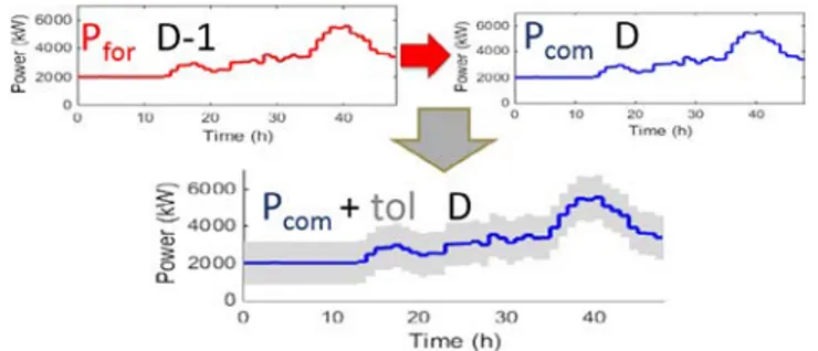
Fig. 1. Commitment assimilated to the forecast power.
to grid services in order to contribute to the whole grid stability [5,20] despite sources intermittence. Adding energy storage systems with corresponding energy management, which are used to create virtual inertia [4,5,32], is one of the major solution to face intermittent character of RES. A lot of studies have been carried out on this topic [10,15,22,24,26,32] for which the main points are the sizing and the management of the storage system. The sizing problem will not be the aim of this paper which is focused on the energy management of the storage device. Inside the energy management issue, many studies can be done as absolute optimization [24] or statistical analysis [10] and different kinds of problems can be processed. Among them, two classes of management strategy using optimization problems can be distinguished:
- Firstly, rule based heuristics without “a priori” on future events are often proposed, as for example with fuzzy logic management [7,12]. Those methods are clearly applicable in real time. Optimal control based approaches (as the example of Pontryagin’s maximization principle) are also used on certain systems with the same characteristics even if actual applicability is often more complex. The first category of problems based on heuristics is clearly the most commonly used especially in the industrial context;
- Secondly, “global optimization” management where all database are known: “a priori” knowledge on past, present and future events is here assumed. Genetic algorithms [6], particle swarm optimization [28] or linear programming (LP) [15,18,22,26], are among the class of methods that can be used which guarantee to reach the global optimum of management performance under modeling assumptions: it gives an “absolute answer” on what should be done at each step. This second class of method is clearly not applicable in real time but may be useful for tuning heuristics or to be used during the sizing process of the system design.
In this article, a linear model for Mixed Integer Linear Programming (MILP) optimization of a smart grid energy management is thus presented. The modeling approach is based on power flow models used to run the energy management of the smart power plant including renewable sources (wind turbines) and a Lithium Ion storage device. The problem statement will be firstly presented. Then a linear model of the system will be proposed with the associated hypothesis. The results obtained over one year of simulation will be exposed and more specifically the impact on some indicators will be presented. The general behavior of the optimal solution will be studied to improve the heuristic management and to develop a new one.
2. Problem setting
The problem is simplified with only one power source (wind turbines, WT) and only one storage technology (Li-Ion). Many studies have been performed on this kind of grids [14,17,19,25] with different storage technologies but on a shorter time horizons: from a few seconds for the frequency control to a few hours. This paper intends to evaluate the proposed method over one year of simulation for a more global evaluation. The concrete goal of this study is to comply with a grid service consisting in a “day ahead power commitment” issue as can be seen in [16,31]. The commitment is generally related to the wind power production forecast; here, in order to focus on the comparison of management strategies, the choice has been made to assimilate power flows for the day ahead forecast (Pfor) with commitment: Pfor(D−1) = Pcom(D) as displayed onFig. 1. A tolerance layer (tol) around the commitment
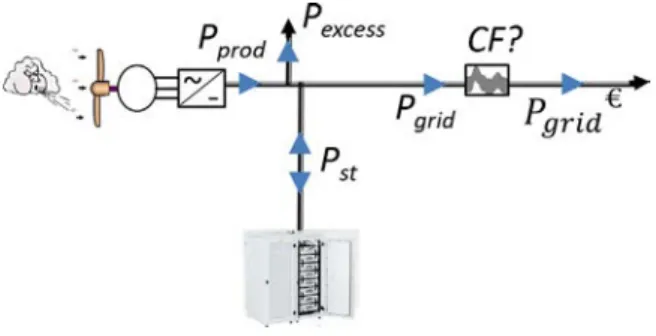
Fig. 2. Power flows.
forecast errors in real time (for the D day) to keep the grid transferred power inside the tolerance band. The study is done in collaboration with industry and the requirements related to smart windfarms with storage for islanded networks are provided by the CRE (https://www.cre.fr) [8]. In the case study, the tolerance (tol) is required to be decreased during the three first years (for a 15 year contract) and this study will deal with the third year which is the hardest in terms of commitment with a tolerance band of 15% of the total sizing power of WT sources.
If the mean power transferred to the grid (Pgrid) does not fulfill this commitment during 1 min, a Commitment
Failure (CF) is triggered and the energy supplied to the grid is not paid for 10 min. Regarding the complexity of system analysis (number of variables and long period of time) simulations have been run with a 10 min time step. Reducing this time step to 1 min will be the purpose of further studies. Preliminary tests showed a low difference between 1 vs 10 min time steps.
2.1. Context of the system
The studied grid connected system is simplified with respect to a real smart grid: both commitment and actually produced powers (Pprod) are not based on physical models: power flow vectors Pprodand Pcomare considered as input
data. At each time step, the management strategy has to decide which part of the produced power will be sent to the grid (Pgrid) and which power will be charged or discharged by the battery (Pst: where Pst> 0 stands for discharge and
Pst< 0 stands for charge). The wind turbine production is normally maximized (MPPT mode) but a power reduction
(curtailment mode) is expectable if excessive production with respect to the power commitment (Pprod> Pcom+tol) is
obtained and if the battery is not able to charge the power excess. For the simulation, this power flow excess (Pexcess) is
considered as dissipated and lost for the economic balance. TheFig. 2displays all corresponding power flows related to the power balance(1)for each time step:
Pprod+Pst=Pexcess+Pgrid (1)
2.2. Comparative study between two EMS
Our objective is firstly to use LP for the energy management optimization in order to find the best trajectory for Pstknowing the whole trajectory of production and forecast data. Pstis the unique unknown variable in(1)that leads
to the grid transfer Pgrid. Pprod and Pcom being known, and by considering the battery limits (state of charge and
maximum charge power), Pexcesscan be determined with respect to the tolerance band (tol).
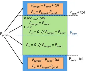
This linear optimization will be compared to a rule-based heuristic method. The heuristic is a management method applicable in real time and which follows rules as shown inFig. 3where SOCLi-Ionrepresents the State Of Charge of
the storage system. This strategy is a good compromise between complying with the day-ahead commitment and an efficient use of the storage system. Ptargetis the power targeted to be transferred to the grid (Pgrid):
Different heuristics have been tested, but all of them had the same rules when Pprodis out of the tolerance band.
In the low production case with Pprod > Pcom−tol: Ptargetis set to the bottom value of the tolerance band and the
difference is discharged with storage (Pst) if enough energy is available in the battery. A CF penalty is triggered in
Fig. 3. Heuristic algorithm.
the band and the difference is stored in the battery within its limits in energy and power. If the one part of the excess power cannot be charged due to storage limits, an excess power (Pexcess) is wasted fulfilling Eq.(1)but no CF penalty
is triggered assuming that wind power production is reduced. This heuristic is a bit more complex when Pprodis inside
the tolerance band:
- if Pcom−tol< Pprod< Pcomthe storage is off;
- if Pcom< Pprod < Pcom+tol and if SOC<60% then Ptarget=Pcom; Pprod−Pcomis then stored in the battery.
This heuristic has been tested with a nonlinear model of the system taking account efficiency of static converters and involving the Tremblay Dessaint model [29] for the battery. In order to run linear programming, a linear derivation has been developed from the nonlinear model, but subsequent results will be tested with the non-linear model. Indeed the point is to assess the ability of the LP to find an optimal storage trajectory (Pst) with the linear model and to keep
a robust performance for the non-linear and more accurate model. 3. Linear model of the power plant
In this part, the model used in the linear programming optimization is presented. The linear model of the battery is given in details, especially the constraints imposed by the grid and the objective function linearized vs decision variables. The model is presented for a discrete simulation of N time steps of ∆t, k being the current step. Equations derived in the following part have to be verified for each step k belonging to the whole profile [1..N].
3.1. Battery linear model
The modeled storage is a Li-Ion battery but its linear model [2] could be easily transposed to any other technology with a simple rated energy Enom. A simple power flow model with charge (ηch) and discharge (ηdis) efficiencies has
been considered to be enough accurate in view of this comparative analysis of EMS performance. Further analysis made with finer models [14,28] have shown that it does not affect the performance ranking of the EMS. In order to get a linear function vs efficiency, the Pstvariable has to be split into 2 parts:
Pst[k] = Pst+[k] + Pst−[k] (2)
where Pst+ is the positive part and Pst− is the negative part of Pstin(2). With this separation the efficiency can be
taking account of the losses: Pbat[k] =ηch.Pst−[k] + Pst + [k] ηdis (3) Different linear constraints related to efficiencies(3)or saturations(4),(5)can be assigned for charge or discharge powers and SOC.
Pbat[k] ≤ Pdis max[k] (4)
Pbat[k] ≥ Pch max[k] (5)
whereηch and Pch max (respectivelyηdis, Pdis max) represent the efficiency and power saturation during the charge
(respectively the discharge) of the battery (absolutes values). The discrete linear implementation of SOC becomes: SOC [k + 1] = SOC [k] +Pbat[k]∆t
Enom
(6) Accordingly to the requirements of the battery provider, the SOC is constrained with saturations to maintain the battery lifespan:
SOCmin=30% and SOCmax=90%
The constraints needed to run the optimization with the context described above are detailed in the next part. 3.2. Linear constraints
Even with this simplified system, several conditions such as “i f Pprod< Pcom–t ol” are not linear and mathematical
tricks have been used. Operators “max” and “min” can be processed as long as they do not operate on decision variables. To solve certain problem binary variables have also to be defined. The Mixed Integer Linear Programming (MILP) approach is used [30].
The first constraint is related to(1)but with linear variables:
Pprod[k] + Pst+[k] + Pst−[k] = Pgrid[k] + Pexcess[k] (7)
All members of this equation are related to decision variables except Pprod[k]. Considering Pgridas a decision variable
with the equality constraint(7) is equivalent to defining its value. Variables P+st/P −
st seem convenient to define the
battery management. But in order to ensure that charge and discharge cannot simultaneously take place, a binary variable D[k] (D[k] = 1 for discharge) is introduced and the following constraints are imposed:
0 ≤ Pst+[k] ≤(ηdisPdis max) × D [k] (8)
max ( −Pch max ηch , −Pprod[k] ) ×(1 − D[k]) ≤ P−st[k] ≤ 0 (9)
If D = 0,(8)ensures P+st =0, i.e. a battery charge operating. If D = 1,(9)ensures P−st =0 imposing the battery to be discharged.
Eq.(7)and the following constraint define Pexcess:
Pgrid[k] ≤ Pcom[k] + tol (10)
Indeed, imposing Pgridbelow the upper band Pexcessfulfills the missing power as explained with(1).
Pexcess[k] ≤ max(Pprod[k] − Pcom[k], 0) (11)
Eq.(11)is an upper bound for Pexcessin order to reduce the search space of the solver.
Saturations of the SOC become for each time step (k ∈[1..N]): − ( k ∑ i =1 Pst+(i) ηdis +ηchPst−(i) ) ≤ Enom
∆t ×(SOCmax−SOCinit) (12)
k ∑ i =1 Pst+(i) ηdis +ηchPst−(i) ≤ Enom
∆t ×(SOCinit−SOCmin) (13)
A constraint on the SOC is added to keep its value at the end of the day equal to the initial value:
SOC(N) = SOCend=SOCinit=50% (14)
This debatable choice has been made in order to decouple planning cycles (i.e. planned days here) from each other. More reasons related to this choice will be detailed in Section4.
Pmissis another variable introduced to help defining the CF condition: CF is a binary variable equal to 1 in case of
commitment failure and 0 otherwise.
Pgrid[k] ≥ Peng[k] − tol − Pmi ss[k] (15)
BIGM × C F [k] ≥ Pmi ss[k] (16)
when Pgridis not inside the tolerance layer, Pmisshas to be non-zero to verify(15). The value of Pmissis not really
relevant, a non-zero value triggers CF=1 thanks to Eq.(16). This method called “Big M” is classically used in LP: the constant BIGM is the big M used to control the value of a binary variable: here CF.
The last constraint is here to prevent the use of the available power to charge the battery during a CF. Indeed, the producer is not paid for the energy provide during a CF period as explained in the introduction. So, during that time, the available power is wasted from the economic point of view.
Pst−[k] ≥ −(1 − C F [k]) × Pprod[k] (17)
This behavior is due to the time step of 10 min used for optimization and which does not allow to define CF more accurately, since its real value is based on the mean value on 1 min followed a possible penalty over 10 min. The trick used in(17)is from the Big M method too which sets CF=1 to impose P−st ≥0 and soP
− st =0.
With the modeling tricks used, a total of 7 variables are necessary to fully derive the problem instead of one (Pbat)
for a nonlinear optimization. Those 7 decision variables are: Pst+, Pst−, Pmiss, Pexcess, Pgrid, CF and D. CF and D being
binary a MILP solver is run. Simulating 24 h with a 10 min time step (144 steps) involves 1008 (7×144) decision variables to be optimized.
The objective function needed to define the optimal solution is detailed in the following section. 3.3. Linear objective function
As explained in introduction, the issue of this linear optimization is to satisfy a grid service for day ahead market and of course to maximize energy producer profits. Multi-objective optimization approaches being sometimes adequate but more complex [11], the choice has been made to minimize a whole cost gathering the process efficiency and the battery use cost. The fulfillment of the grid service is thus shifted in a monetary cost from the CF penalty consequence. The cost function has been decomposed into 4 parts:
−A first part includes the “deviation cost” due to the CF: the producer is not paid for power to the grid (Pgrid) if
CF=1, the associated cost being defined as:
Costdev[k] = FIT × C F [k] × Pgrid[k]∆t (18)
where FIT denotes the Feed in Tariff in [e/kWh]. However, Pgridand CF are both decision variables so this expression
is not in accordance with the linear programming. If CF = 1, then Pgridis below the lower limit of the tolerance layer
so Pexcess= 0. The constraint(16)prevents against any charge and there is no interest to discharge the battery if we are
not remunerated for the energy provided so Pst= 0. Pgrid= Pprodin the case of CF = 1 can be deduced from(1), where
Pprodis an input data of the problem and the expression of Costdevbecomes:
Costdev[k] = FIT × CF [k] × Pprod[k]∆t (19)
−A second part consists in the ‘’wasting cost” where energy is lost with Pexcess:
Costwas[k] = FIT × Pexcess[k]∆t (20)
−the third and fourth parts represent the costs due to the battery use, especially related to losses and life cost of this storage device. The third part related to efficiency is similar as previously:
Costη Li-I on[k] = F I T [ (ηch−1) Pst−[k] + 1 −ηdis ηdis Pst+[k] ] ∆t (21)
The importance of separating Pstto express this cost linearly with decision variables is shown here. Finally, the fourth
part related to the life cost of the battery is based on the maximum exchangeable energy Eexc-max[kWh] as detailed
in [11]. This last model calculates a percentage of the lifespan already consumed which is multiplied by the cost of one battery CostLi-I on to obtain the life cost during battery use. This “lifetime model” is based on the cycle to
failure curve [3] provided in datasheets which specifies the battery aging with respect to the DOD. This approach is relevant if thermal operation of the battery shelter is controlled as in our case study. A more accurate model counting cycles during operation is sometimes used but this simplification proposed by [1] based on the exchanged energy with the battery during its operation is enough accurate in order to assess the performance of an EMS, especially for comparing performance of several strategies. This model is then considered as enough accurate to show a tendency and will not allow the optimizer to use the battery without affecting the cost function Furthermore, this simplification allows deriving an analytical model which can be linearized as:
Costlife[k] = CostLi-I on.
( Pst+[k] ηdis −ηchPst−[k] ) ∆t Eexc−max (22) The total cost function is obtained by adding all considered costs:
Costt ot[k] = Costdev[k] + Costwas[k] + Costη Li-I on[k] + Costlife[k] (23)
The MILP solver minimizes this total cost and seeks the optimal trajectory for Pst. Results obtained are exposed in
the following and last part of this paper. 4. Simulations results
Results are obtained using the following method:
We first used GLPK as a unique solver but then switched to CPLEX which is much faster. One year of simulation nearly take 3 min of CPU time. Once all the results (Pbattrajectory) are obtained, the system simulation is performed
on the non-linear model and the cost criteria are extracted. Results obtained over a full year with a succession of 365 day MILP optimizations raise several issues. In comparison, one year is also simulated with the heuristic algorithm for energy management. The comparative analysis is based on several criteria:
−Cost: as shown in Section3.3(Eq.(18)to(23)) but calculated with the non-linear model.
−Gain: the complementary function of the cost represents the money earned by the energy producer:
Gai n =FIT(1 − C F) Pgrid.∆t − Costlife (24)
Also expressed as:
Gai n =FIT × Pprod∆t − Costt ot (25)
where the complementarity is shown. The Cost indicator allows us to optimize the Gain with a greater sensibility. − Commitment Failure is a relevant criterion for grid services. Indeed agreements are made to increase the penetration rate of intermittent renewable sources with reliable and stable operation of islanded grids.
4.1. Model adaptation
The heuristic management strategy is a step by step algorithm which can be applied over a full year of simulation without any problem. The linear optimization is done day by day to be closer to the real commitment problem. In order to be able to simulate one full year, the SOC continuity between two successive days has to be ensured, which is related to(14): SOCend = SOCinit. But even if this constraint is satisfied with the linear model it may be slightly
different with the non-linear. The choice has been to calculate the gain available with a ∆SOC = SOCend−SOCinit
as if this energy would be sold at the FIT price and then would be added to the global gain:
Gai nSOC =FIT(SOCend−SOCinit) Ebat tot (26)
This choice is questionable, but differences between the linear vs non-linear models were not important so this way of correction was seen as relevant to our study. If this correction is not done, the complementarity between gain and cost is not respected anymore.
Table 1
Comparison between linear optimization and heuristic management. Heuristic management Linear optimization Relative difference Gain 4 018 ke 4 134 ke 3% Cost 535 ke 418 ke 28% CF 8.3% 5.8% 30%
The following results presented are obtained with 4 wind turbines of 2MW each and 3 battery shelters (SAFT batteries model Intensium Max 20M) of 580 kWh each (Pchmax=600kW and Pdismax=1100kW per battery). This
represents a total estimated investment of 14 900 ke(used for the economic model). Detailed economic data cannot be provided due to confidential issues.
4.2. Cost comparison
The costs related to the use of Lithium Ion storage are gathered:
Costst o=Costη Li I on+Costlife (27)
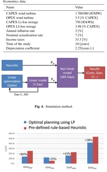
Simulations obtained over one year show the ability of the MILP to provide better results than a heuristic even on the same non-linear model. The MILP uses battery twice as much as the heuristic management to reduce wasted and deviation costs.Fig. 5well emphasizes this issue.
Underusing the battery causes a significant increase of the other parts of the cost function. If only the deviation and storage costs are analyzed, it seems that the battery just has to be used more in a far-sighted approach. But the fact that the wasted cost is increased with heuristic shows that the battery was more often overloaded than for MILP management.
4.3. Other comparison on gain and CF
One goal of the study is to focus on the energy producer point of view for which gain is the most important criterion. Furthermore, the grid point of view is another goal of this study, so that the CF will also be a relevant criterion (see
Table 1).
The MILP optimization improves all criteria. The sensitivity of the cost function with regard to the gain is clearly demonstrated here. A significant increase of 28% has been made on the cost but only 3% on the gain. This latter gives the total amount of money theoretically earned during one typical year. This result shows the improvement potential on the gain which cannot be more than 10% “even if the cost would be zero” which would correspond with a perfect production forecast. Results on the CF factor show the MILP capability to also enhance the production forecast of this smart wind power plant, the global CF over one year being almost reduced by 30%. It should be noted that the global CF is reduced, but not on every single simulation step. For some particular days, the LP optimizer is able to reduce the cost by slightly increasing the CF. This particular case occurs because the associated deviation cost is weighted by Pgrid. This aspect is not absurd even on the grid point of view: indeed CF is all the more problematical when the
energy producer does not comply with a high power commitment.
The power flow simulation over one year has been extended to a 10 year economical study with the calculation of Levelized Cost Of Energy (LCOE), which represents the minimal price of energy to refund the initial investment, and the Net Present Value (NPV) which shows a measure of the project’s profitability. The method used is presented in [27] and an example can be seen in [21].
NPV and LCOE are more significant indicators than the cost which is more convenient for the linear optimization. The results over a longer range (10 years) are positive. The linear optimization shows a great improvement with 13% on the NPV and 4% on the LCOE. Data used for those calculations are summarized inTable 3.
Table 2
10 years economics results. Heuristic management Linear optimization Relative difference NPV 7 074 ke 7 964 ke 13%
LCOE 113e/MWh 108.5e/MWh 4%
Table 3 Economics data.
Name Value
CAPEX wind turbine 1 700 000 [e/MW] OPEX wind turbine 3.5 [% CAPEX] CAPEX Li-Ion storage 750 [e/kWh] OPEX LI-Ion storage 3.98 [% CAPEX] Annual inflation rate 2 [%]
Nominal actualization rate 7 [%]
Income taxes 33.3 [%]
Time of the study 10 [years] Depreciation coefficient 2.25/years [-]
Fig. 4. Simulation method.
Fig. 5. Cost comparison for both optimization approaches of energy management.
4.4. Day by day analysis
The cost deviation between the LP optimal planning and the rule-based heuristic is now analyzed for each day of the simulated year. This will show if the optimal LP solver is capable of reducing each day cost or if the difference is due to critical days which concentrate all the improvement.
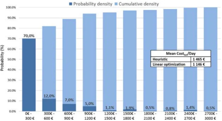
Fig. 6shows a reconstruction of the probability density and the cumulative density functions associated with this cost deviation by considering a day by day comparison between the heuristic and linear programming optimization.
Fig. 6. Cost deviation between the optimal LP planning and the Heuristic on the data set.
Table 4
Linear optimization with different SOCinit. Linear optimization SOCinit(%) 30% 40% 50% 60% 70% 80% 90% Costtot(ke) 439 425 418 416 415 416 419 Coststo(ke) 122 123 122 122 121 123 123 Costdev(ke) 157 143 137 135 132 131 131 Costwas(ke) 160 159 159 159 162 162 165
The figure shows that for 70% of the days the improvement is less than 300e. Indeed, for a lot of days, forecasts are very low which reduces the impact of the energy management in the global cost. If the power forecast is below half the size of the tolerance layer, Pcom =Pfor would induce a negative part of the tolerance layer. In this case the
tolerance layer is set at the minimum from 0 to 30% of the installed power (tolerance layer being +/- 15%) which gives more flexibility than usual and prevent from any CF. For 30% of the days, the improvement is beyond 300ewhich is quite important compared to the mean total cost per day over the year.
As previously mentioned (Fig. 4), one important difference between both management methods resides in the fact that the heuristics plays the 365 days in a row while the LP separately plays each of the 365 days before being assembled. To ensure the continuity of the SOC in that case, the constraint(14)is applied. One of the consequences is that each day of the optimal solution begin with SOCinit = 50% while this level depends on what happened the
previous day for the heuristic. A study of the impact of SOCinithas been realized to analyze the day by day difference
between linear programming optimization and heuristic. 4.5. Impact ofSOCinit
Several simulations have been performed with different values on the SOCinit constraint. The results are
summarized inTable 4.
It should be reminded that 30% and 90% are the low and high limits considered in the energy management for the storage system.Table 2results show that the impact of SOCinitis low. Indeed, except when the constraint is set on a
saturation level the difference of costs is negligible which comforts our previous hypothesis. 4.6. One particular Day analysis
One particular day (low level of production vs forecast power) where the cost difference is quite important is analyzed. Other typical days studied but not presented showed the same difference of behavior between both strategies.
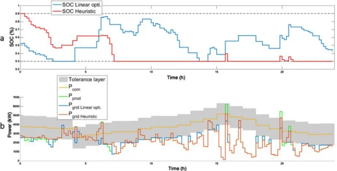
Fig. 7. Comparison between LP and Heuristic strategy a. SOC b. Power flows.
Table 5
Costs’ details for Heuristic and linear optimization.
Day 133 Storage cost Wasted Cost Deviation cost Total cost
Heuristic 297e 0e 5 235e 5 532e
Linear optimization 659e 0e 2 528e 3 188e Difference −362e 0e 2 707e 2 344e
Fig. 7shows the variations of SOC with both strategies for a 24 h sample and the corresponding grid power flow. In the first part of the day, the difference between both strategies is due to the SOCinitwhich is favorable to the
heuristic. This results in a similar behavior of both management strategies which use the stored energy to prevent CF. After 7 a.m. the heuristic trajectory is locked due to the SOC saturation at the lower limit whereas the LP optimal planning is capable of exploiting the storage over the whole SOC range reducing the commitment failure when the forecast error is higher. It should be noted, contrary to the heuristic management, that LP optimal planning charges the battery even in the low part of the tolerance layer in order to have back up energy and prevent further CF.Table 5
details the different parts of the Costt otfor this particular day:
Those results show that the battery has to be used more intensively than for the current heuristic. The storage cost is a bit higher in the linear optimal solution in order to reduce a lot the C.F. However, knowing the future production during the day allows the MILP to use the battery exactly when necessary. These trends are useful for future heuristic tuning as it will be developed in the next part of this article.
5. New heuristic deduced from the behavior of the lp optimal planning
The LP optimization has been developed in the scope of two different purposes. It can be firstly used during the design step as an energy management for sizing the smart wind power plant components [23]. Secondly, as an “ideal” reference, it can also be exploited for improving rule-based heuristics or optimal control laws without a priori on the future for real time applicability.
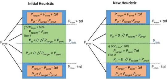
Fig. 8shows the new heuristic developed compared with the initial one.
The rules outside the tolerance layer are the same for both heuristics but the behavior inside the tolerance layer is completely opposite. Indeed the initial heuristic was based “on common sense” to charge the battery in case of overproduction inside the tolerance layer, and directly transfer the produced power through the grid in case of under
Fig. 8. New Heuristic algorithm.
Table 6
Comparison of the costs obtained with the initial and new heuristics for the considered year. Storage cost Wasted cost Deviation cost Total cost Initial Heuristic 55 ke 227 ke 252 ke 535 ke New Heuristic 66 ke 224 ke 221 ke 511 ke
Difference −11 ke 3 ke 31 ke 24 ke
production. The analysis of the data set revealed “a bias” between wind forecast and production: in particular, a situation of underproduction is most likely to happen again in the following step times increasing the CF occurrence probability. Therefore, in case of a production lower than the forecast the choice is made to charge the battery with the new heuristic in order to be able to prevent future CF by using this stored power. The threshold on the SOC (SOCLi I on < 50%) is here in order to prevent overusing the battery. The behavior in the upper part of the tolerance
layer is symmetrical. In case of overproduction, the storage is not used so as to absorb this overproduction and avoid wasted power. This relation between Pprodand Pf or could be justified by persistence effects [13].
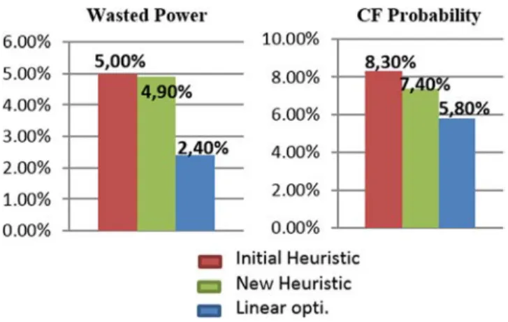
One cannot conclude on the optimality of this second heuristic but it clearly outperforms the initial one as shown inTable 4andFig. 9. In this figure, the wasted power is expressed as a percentage in relation to the power produced, and the CF probability is calculated over the whole year duration. The LP optimization has also been added as the ideal reference (seeTable 6).
The changes implemented in the new heuristic strategy have the desired effect on the costs. First of all, the total cost is reduced by almost 5%. The behavior of the new heuristic is closer to the optimal dispatching resulting from the LP optimization. The battery is more efficiently used with regard to the commitment failure reduction. Even if the wasted cost is not strongly reduced, it remains better with the new heuristic.
Wasted power and CF are complementary quantities and it was easy to find a heuristic which reduce one but increase the other one (by playing with the SOC threshold for example). The power of this new heuristic is to be able to reduce both which shows the fundamental improvement.
6. Conclusion
˙In this paper, a smart wind power plant composed by a wind farm and a Li-ion battery is studied in the context of island networks. A linear model has been developed to be used with a MILP optimization solver. A comparative study has been made with a rule based heuristic method: even if this latter is applicable in real time the comparison shows that heuristic may be significantly improved. The ability of a linear programming to give optimal results on linear model but exploitable on a non-linear and more accurate model has been proven. Those results have been used to improve decision making for heuristic algorithms. A second heuristic algorithm has been developed based on LP
Fig. 9. Comparison between initial and new Heuristic.
behavior showing major improvements in particular by reducing the CF without increasing the wasted power by using the storage system more efficiently. Those results will be used in further studies investigating the co-optimization of component sizing and energy management in the smart wind power plant.
Acknowledgment
This research benefited from the support of the Cellule Energy of the CNRS, France. References
[1] D. Abbes, A. Martinez, G. Champenois, Life cycle cost, embodied energy and loss of power supply probability for the optimal design of hybrid power systems, Math. Comput. Simulation 98 (2014) 46–62.
[2] M.J.M. Al Essa, Management of charging cycles for grid-connected energy storage batteries, J. Energy Storage 18 (2018) 380–388.
[3] Battery datasheet,https://www.saftbatteries.com/products-solutions/products/intensium⃝R-max-megawatt-energy-storage-system(download the “Li-ion battery life - Technical sheet”).
[4] H.P. Beck, R. Hesse, Virtual synchronous machine, in: 2007 9th international conference on electrical power quality and utilisation, 2007, pp. 1–6.
[5] M. Benidris, J. Mitra, Enhancing stability performance of renewable energy generators by utilizing virtual inertia, in: 2012 IEEE Power and Energy Society General Meeting, 2012, pp. 1–6.
[6] C. Chen, S. Duan, T. Cai, B. Liu, G. Hu, Optimal allocation and economic analysis of energy storage system in microgrids, IEEE Trans. Power Electron. 26 (10) (2011) 2762–2773.
[7] V. Courtecuisse, J. Sprooten, B. Robyns, M. Petit, B. Francois, J. Deuse, A methodology to design a fuzzy logic based supervision of Hybrid Renewable Energy Systems, Math. Comput. Simulation 81 (2) (2010) 208–224.
[8] CRE, ‘Cahier des charges de l’appel d’offres n◦332689-2010-FR portant sur des installations éoliennes terrestres de production d’électricité en Corse, Guadeloupe, Guyane, Martinique, à la réunion, à Saint-Barthélemy et à Saint-Martin’, p. 14, 2010.
[9] Guadeloupe energetic politic, https://www.guadeloupe-energie.gp/politique-energetique/strategie-regionale/vers-lautonomie-energetique-de-la-guadeloupe/.
[10] P. Haessig, B. Multon, H.B. Ahmed, S. Lascaud, P. Bondon, Energy storage sizing for wind power: impact of the autocorrelation of day-ahead forecast errors, Wind Energy 18 (1) (2015) 43–57.
[11] D. Hernandez-Torres, C. Turpin, X. Roboam, B. Sareni, Techno-economical optimization of wind power production including Lithium and/or Hydrogen sizing in the context of the day ahead market in island grids. Elsevier MATCOM journal (Mathematics and Computers in Simulation), Electrimacs2017 special issue, 2017.
[12] K.-S. Jeong, W.-Y. Lee, C.-S. Kim, Energy management strategies of a fuel cell/battery hybrid system using fuzzy logics, J. Power Sources 145 (2) (2005) 319–326.
[13] N. Korprasertsak, T. Leephakpreeda, Comparative investigation of short-term wind speed forecasting models for airborne wind turbines, in: 2017 8th International Conference on Mechanical and Aerospace Engineering, ICMAE, 2017, pp. 451–454.
[14] G. Mandic, A. Nasiri, E. Ghotbi, E. Muljadi, Lithium-ion capacitor energy storage integrated with variable speed wind turbines for power smoothing, IEEE J. Emerg. Sel. Top. Power Electron. 1 (4) (2013) 287–295.
[15] A. Maroufmashat, M. Fowler, S. Sattari Khavas, A. Elkamel, R. Roshandel, A. Hajimiragha, Mixed integer linear programing based approach for optimal planning and operation of a smart urban energy network to support the hydrogen economy, Int. J. Hydrog. Energy 41 (19) (2016) 7700–7716.
[16] E.S. Matee, G. Radman, Determination of optimum economic power commitment by wind farms equipped with energy storage system, in: IEEE Southeastcon 2014, 2014, pp. 1–6.
[17] L. Miao, J. Wen, H. Xie, C. Yue, W.J. Lee, Coordinated control strategy of wind turbine generator and energy storage equipment for frequency support, IEEE Trans. Ind. Appl. 51 (4) (2015) 2732–2742.
[18] H. Morais, P. Kádár, P. Faria, Z.A. Vale, H.M. Khodr, Optimal scheduling of a renewable micro-grid in an isolated load area using mixed-integer linear programming, Renew. Energy 35 (1) (2010) 151–156.
[19] S. Nasri, S. Ben Slama, I. Yahyaoui, B. Zafar, A. Cherif, Autonomous hybrid system and coordinated intelligent management approach in power system operation and control using hydrogen storage, Int. J. Hydrog. Energy 42 (15) (2017) 9511–9523.
[20] N. Nguyen, J. Mitra, An analysis of the effects and dependency of wind power penetration on system frequency regulation, IEEE Trans. Sustain. Energy 7 (1) (2016) 354–363.
[21] M. O’Connor, T. Lewis, G. Dalton, Techno-economic performance of the Pelamis P1 and Wavestar at different ratings and various locations in Europe, Renew. Energy 50 (Supplement C) (2013) 889–900.
[22] R. Rigo-Mariani, B. Sareni, X. Roboam, Fast power flow scheduling and sensitivity analysis for sizing a microgrid with storage, Math. Comput. Simul. 131 (Supplement C) (2017) 114–127.
[23] R. Rigo-Mariani, B. Sareni, X. Roboam, Integrated optimal design of a smart microgrid with storage, IEEE Trans. Smart Grid 8 (4) (2017) 1762–1770.
[24] R. Rigo-Mariani, B. Sareni, X. Roboam, C. Turpin, Optimal power dispatching strategies in smart-microgrids with storage, Renew. Sustain. Energy Rev. 40 (2014) 649–658.
[25] R.H.L. Rodriguez, I. Vechiu, S. Jupin, S. Bacha, Q. Tabart, E. Pouresmaeil, A new energy management strategy for a grid connected wind turbine-battery storage power plant, in: 2018 IEEE International Conference on Industrial Technology, ICIT, 2018, pp. 873–879.
[26] M. Sechilariu, B. Wang, F. Locment, Power management and optimization for isolated DC microgrid, in: Automation and Motion 2014 International Symposium on Power Electronics, Electrical Drives, 2014, pp. 1284–1289.
[27] W. Short, D. Packey, T. Holt, A Manual for the Economic Evaluation of Energy Efficiency and Renewable Energy Technologies, vol. 95. 1995.
[28] J. Soares, M. Silva, T. Sousa, Z. Vale, H. Morais, Distributed energy resource short-term scheduling using Signaled Particle Swarm Optimization, Energy 42 (1) (2012) 466–476.
[29] O. Tremblay, L.-A. Dessaint, Experimental validation of a battery dynamic model for EV applications, World Electr. Veh. J. 3 (1) (2009) 1–10.
[30] Robert J. Vanderbei, Linear Programming: Fundations and Extensions, 2001 Vol 2 Chapter 23.
[31] C. Wang, et al., Day-ahead unit commitment method considering time sequence feature of wind power forecast error, Int. J. Electr. Power Energy Syst. 98 (2018) 156–166.
[32] M. Zaibi, G. Champenois, X. Roboam, J. Belhadj, B. Sareni, Smart power management of a hybrid photovoltaic/wind stand-alone system coupling battery storage and hydraulic network, Math. Comput. Simul. (2016).