Any correspondence concerning this service should be sent
to the repository administrator: [email protected]
This is an author’s version published in:
http://oatao.univ-toulouse.fr/22492
Official URL
DOI : https://doi.org/10.1109/SSP.2018.8450758
Open Archive Toulouse Archive Ouverte
OATAO is an open access repository that collects the work of Toulouse
researchers and makes it freely available over the web where possible
To cite this version:
Abry, Patrice and Wendt, Herwig and
Didier, Gustavo Detecting and Estimating Multivariate Self-Similar
Sources in High-Dimensional Noisy Mixtures. (2018) In: IEEE
Workshop on statistical signal processing (SSP 2018), 10 June 2018
- 13 June 2018 (Freiburg, Germany).
DETECTING AND ESTIMATING MULTIVARIATE SELF-SIMILAR SOURCES
IN HIGH-DIMENSIONAL NOISY MIXTURES
Patrice Abry
1, Herwig Wendt
2, Gustavo Didier
3 1Univ Lyon, Ens de Lyon, Univ Claude Bernard, CNRS, Laboratoire de Physique, Lyon, France.
2IRIT, CNRS (UMR 5505) , Universit´e de Toulouse, France.
3Math. Dept., Tulane University, New Orleans, USA.
ABSTRACT
Nowadays, because of the massive and systematic deployment of sensors, systems are routinely monitored via a large collection of time series. However, the actual number of sources driving the tem-poral dynamics of these time series is often far smaller than the number of observed components. Independently, self-similarity has proven to be a relevant model for temporal dynamics in numerous applications. The present work aims to devise a procedure for identi-fying the number of multivariate self-similar mixed components and entangled in a large number of noisy observations. It relies on the analysis of the evolution across scales of the eigenstructure of multi-variate wavelet representations of data, to which model order selec-tion strategies are applied and compared. Monte Carlo simulaselec-tions show that the proposed procedure permits identifying the number of multivariate self-similar mixed components and to accurately esti-mate the corresponding self-similarity exponents, even at low signal to noise ratio and for a very large number of actually observed mixed and noisy time series.
Index Terms— multivariate self-similarity, operator fractional Brownian motion, wavelet spectrum, model order selection
1. INTRODUCTION
Context: multiple sensors versus few sources. Recent techno-logical developments have permitted the massive production of low cost sensors with low cost deployment, as well as the easy storage and processing of large amounts of data, the so-called data deluge. Therefore, it is very common that one same system is monitored by a large number of sensors producing multivariate and dependent data, i.e., a large number of time series recorded together, whose joint tem-poral dynamics contain information about the system under scrutiny. This is the case in numerous applications that are very different in nature, such as macroscopic brain activity, where the number of ob-served time series ranges from hundreds (MEG data) to several tens of thousands (fMRI data), cf., e.g., [1, 2], or in meteorology and climate studies, where the use of large numbers of measured com-ponents has become standard (e.g., [3]). However, the number of actual mechanisms, or sources, driving the spatio-temporal dynam-ics of one single system is usually far smaller than the number of recorded time series (sparsity). Therefore, it has become a research trend in data analysis to develop methods for identifying the actual number of sources driving the dynamics of a given system, as well as to extract the information provided by these sources from the usu-ally noisy observations.
Work supported by Grant ANR-16-CE33-0020 MultiFracs. G.D. was partially supported by the ARO grant W911NF-14-1-0475.
Context: multivariate self-similarity. Scale-free dynamics has proven to be a useful concept to model real-world data produced from numerous applications in several branches of science and tech-nology (e.g., [4, 5] and references therein). In essence, the scale-free paradigm assumes that temporal dynamics are not governed by one or a few characteristic time scales but, instead, by a large continuum of time scales that jointly contribute to the temporal dependencies. Self-similarity provides a formal, versatile model for scale-free dy-namics [6]. In a stochastic processes framework, fractional Brow-nian motion (fBm) [7] has been widely and successfully used to model real-world data characterized by scale-free dynamics. While the modeling of the latter in applications has remained so far based on the univariate fBm model, a multivariate extension called operator fractional Brownian motion (ofBm) was recently proposed [8–11] to permit their modeling in a multivariate time series setting [12]. The availability and potential of this multivariate self-similarity model for describing real-world data immediately raises a first yet critical question: how many different self-similar components actually exist amongst the possibly very large number of time series recorded by sensors?
Related work. The general issues of identifying the number of actual sources in potentially high-dimensional multivariate signals, and of characterizing them from noisy observations, has continu-ously been addressed in statistical signal processing over the years. Often embedded in the general themes of dimensionality reduction, source separation [13], or model order selection and system identi-fication [14–17], numerous technically distinct solutions were pro-posed in theory and widely used in applications. Examples include principal component analysis (PCA), factor analysis, sparse graphi-cal Gaussian models, etc. (cf., e.g., [18]). Independently, a multivari-ate wavelet variance eigenvalue-based representation of multivarimultivari-ate self-similarity was recently put forward and studied [12]. Notably, it was shown to lead to efficient and robust estimation of self-similarity exponents in intricate multivariate settings [19]. Notwithstanding significant success in applications, none of the classical dimension reduction tools takes explicitly into account multivariate scale-free dynamics (see [20, 21] for exceptions). Thus, there is a great paucity of methodological and practical data modeling tools that are both in-herently multivariate and scale-free analytical.
Goal, contributions and outline. The present work is a first con-tribution aiming at identifying and characterizing multivariate self-similar components embedded in a large set of noisy observations. It relies on ofBm, whose definition and properties are recalled in Sec-tion 2.1, as well as on the recently proposed multivariate eigenvalue wavelet representation, detailed in Section 2.2. The model, com-prising a high-dimensional mixture of low-dimensional multivariate self-similar sources in additive noise, is described in Section 3.1.
Section 3.2 contains the proposed model order selection procedure. It relies on information theoretic tools constructed and studied in different contexts [15–17] and adapted here to the multivariate and multiscale eigenvalue wavelet representation of the noisy observa-tions. Using large size Monte Carlo experiments, the performance of the devised model order selection methods is assessed in com-putational practice for various instances of ofBm (combinations of scaling exponents, mixing matrices and covariance), number of ac-tual self-similar components versus observed time series, noise level and sample size. The method’s performance, depicted and analyzed in Section 4, is shown to be promising in its ability to identify the number of ofBm components amidst noisy observations and to esti-mate the corresponding multiple self-similarity exponents.
2. OPERATOR FRACTIONAL BROWNIAN MOTION AND WAVELET ESTIMATION OF SCALING EXPONENTS 2.1. Operator fractional Brownian motion
The present work makes uses of ofBm for modeling multivariate self-similar structures in real-world data, whose definition and prop-erties are briefly recalled here (the interested reader is referred to [10] for the most general definition and properties of ofBm). Let BH,Σ(t) = !BH1(t), . . . , BHM(t)
"
t∈Rdenote a collection ofM possibly correlated fBm components defined by their individual self-similarity exponents H = (H1, . . . , HM), 0 < H1 ≤ . . . ≤ HM < 1. Let Σ be a pointwise covariance matrix with entries (Σ)m,m′ = σmσm′ρm,m′, where σ2mare the variances of the com-ponents and ρm,m′ their pairwise Pearson correlation coefficients.
We define ofBm as the stochastic processBP,H,Σ(t)! P BH,Σ(t), whereP is a real-valued, M × M invertible matrix that mixes the components (changes the scaling coordinates) ofBH,Σ(t). In this case, ofBm consists of a multivariate Gaussian self-similar process with stationary increments. Moreover, it satisfies the (operator) self-similarity relation
{BP,H,Σ(t)}t∈R
fdd
={aHBP,H,Σ(t/a))}t∈R, (1)
∀a > 0, with matrix exponent H = P diag(H)P−1, termed Hurst matrix parameter,aH! #+∞
k=0logk(a)Hk/k!, where fdd
= stands for the equality of finite dimensional distributions. It is well documented that the scaling exponentsH (Hurst eigenvalues) and the covariance matrixΣ cannot be chosen independently [10, 22]. For simplicity, hereafter we denote
Y (t)! BP,H,Σ(t). 2.2. Wavelet based scaling exponent estimation
Multivariate wavelet transform. The multivariate DWT of
the multivariate process {Y (t)}t∈R is defined as DY(2j, k) ! (DY1(2 j, k), . . . , D YM(2 j, k)), ∀k ∈ Z, ∀j ∈ Z, and m ∈ {1, . . . , M }, with DYm(2 j, k) ! %2−j/2ψ(2−jt − k)|Y m(t)', where ψ0denotes the mother wavelet. For a detailed introduction to wavelet transforms, interested readers are referred to, e.g., [23]. Multivariate self-similarity in the wavelet domain. It can be shown that the wavelet coefficients {DY(2j, k)}k∈Z satisfy the (operator) self-similarity relation [12, 19]
{DY(2j, k)}k∈Zfdd={2j(H+
1
2I)DY(1, k)}k∈Z, (2)
for every fixed octavej. When P = I (no mixing), the (canoni-cal) components of ofBm are generally correlated fBm processes. In
this case,M -variate (operator) self-similarity in the wavelet domain boils down toM entrywise self-similarity relations [22]
{DY1(2 j , k), . . . , DYM(2 j , k)}k∈Z fdd ={2j(H1+12)DY 1(1, k), . . . , 2 j(HM+12)DY M(1, k)}k∈Z. (3)
Estimation of H. Extending univariate wavelet analysis, it is natural to consider the empirical wavelet spectrum (variance), which is given by theM × M matrices
SY(2j) = 1 nj nj $ k=1 DY(2j, k)DY(2j, k)∗, nj= N 2j, whereN is the data sample size. Proceeding as in the univariate setting leads to the estimators [22]
ˆ Hm(U )= % j2 $ j=j1 wjlog2SY,(m,m)(2j) & ' 2 −1 2, ∀m. (4)
Starting from (3), namely, when there is no mixing (P = I), ˆHm(U ) is expected to be a good estimator ofHm. However, starting from (2), i.e., a general mixing matrixP (non-canonical coordinates) and Hurst matrix parameterH, it is clear that this is no longer the case (cf., [12, 19] and Section 4.1 for further discussions).
These observations lead to the definition of an estimator forH that is relevant in the general setting of non-diagonalP using the eigenvaluesΛY(2j) ={λ1(2j), . . . , λM(2j)} of SY(2j). The es-timators ˆH = ( ˆH1, . . . , ˆHM) for (H1, . . . , HM) are defined by means of weighted linear regressions across scales2j1≤ a ≤ 2j2
ˆ Hm= % j2 $ j=j1 wjlog2λm(2j) & ' 2 −1 2, ∀m. (5)
It is shown both theoretically and in practice that ˆH benefits from satisfactory performance (consistency, asymptotic normality), see [12, 19].
3. MODEL ORDER SELECTION FOR HIGH-DIMENSIONAL NOISY MIXTURES 3.1. High-dimensional noisy observations
To model the embedding of ofBmY in a large set of noisy observa-tionsZ, let now W denote a matrix of size L × M , L ≥ M , with full rankM , and let N (t) =!N1(t), . . . , NL(t)"t∈Rbe a collec-tion ofL independent vectors, each consisting of i.i.d. standardized Gaussian variables. TheL observed noisy time series are modeled as
Z(t)! W Y (t) + σNN (t), (6)
where σN2 controls the variance of the noise. Adhering to the con-vention thatW and P are normalized such that W P has rows with unit norm, the Signal-to-Noise Ratio (SNR) is defined as
SNR! M $ m=1 σm ' (LσN) (7)
3.2. Model order selection procedure
The proposed procedure relies on the eigenstructure of the empir-ical wavelet spectra SZ(2j) of the multivariate wavelet represen-tation of the L-variate observations Z. It is obvious that, in the absence of noise (i.e., SNR = +∞), SZ(2j) has rank M for all scales2j (as long asn
j > M ). Conversely, when noise is added (SNR < +∞), SZ(2j) has rank L. Hence, heuristically speak-ing, when the SNR is sufficiently large, SZ(j) possess L − M small eigenvalues corresponding to noise, andM (large) eigenval-ues that correspond to the hidden ofBm components. Then,M can be estimated by using classical eigenvalue-based model order selec-tion criteria, ˆM = φN((λ1, . . . , λL)), such as Akaike’s Informa-tion Criterion (AIC) or Minimum DescripInforma-tion Length (MDL), see, e.g., [15–17] for details and more references.
However, in the context of multivariate self-similarity, wavelet spectra matricesSZ(2j) are available corresponding to each octave and must be combined. To this end, we study two strategies, which we refer to as majority vote (MV) and rescaled-average (RS). As a common preprocessing step, the wavelet spectra SZ(2j) of the L-variate observations Z and their eigenvalues ΛZ(2j) of SZ(2j) are computed, estimates ˆHlare obtained using (5), and the rescaled eigenvalues (ΛZ(2j))l ! 2−2j ˆHl(ΛZ(2j))l, l = 1, . . . , L are computed. The rationale behind ΛZ(2j) is the use the multivari-ate self-similarity of the sources for reducing the variance of their eigenvalues at each scale and for enabling averaging across scales.
For some φN, the model order selection strategies are defined as follows.
MV: A model order estimate ˆM (j) is computed for ΛZ(2j) ˆ
M (j) = φnj(ΛZ(2
j))
for each scalej. Then the scale-wise estimates ˆMjare com-bined by majority vote (where 1() is the indicator funtion)
ˆ MM V = arg maxm=0,...,L j2 $ j=j1 1( ˆM (j) − m). RS: The rescaled eigenvaluesΛZ(2j) are averaged across scales
ΛZ= $j2
j=j1Λ
Z(2j).
A model order estimate ˆM is computed from the averages ˆ
MRS= φN(ΛZ).
For both strategies, the AIC classical model order selection is used φN(Λ) = arg min
k −N (α − k) log!g(k)/a(k)" + k(2α − k), (8) where α= min(L, N ), a(k), g(k) are the arithmetic and geometric mean of thek smallest values of Λ, respectively.
Once the number of ofBm components ˆM is estimated, a scaling exponents vector( ˆH1, . . . , ˆHMˆ) can be computed using the estima-tion procedure described in (5), applied to the ˆM largest values of ΛZ(2j), where ΛZ(2j) denotes the eigenvalues of SZ(2j).
4. PERFORMANCE ASSESSMENT
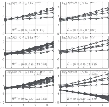
We apply the ofBm model order selection and parameter estima-tion procedure to1000 independent realizations of ofBm with M = 4 components of length N = 214using various SNR values, as defined in (7). We consider4 different sizes for the mixing ma-trix W , L ∈ (10, 20, 50, 100); W is drawn at random for each realization of ofBm and normalized such thatW P has unit norm rows. The ofBm parameters are set toH = (0.2, 0.5, 0.7, 0.9) and Σ = Toeplitz(1, 0.2, 0.2, 0.3). We use the Daubechies wavelet with Nψ= 2, and pick (j1, j2) = (4, 9) in (5). 2 4 6 8 -10 -5 0 5 j log2S(2j)/2 − j/2 for P−1Y ˆ H(U )= (0.17, 0.5, 0.71, 0.9) 2 4 6 8 -10 -5 0 5 j log2Λ(2j)/2 − j/2 for P−1Y ˆ H = (0.18, 0.5, 0.7, 0.88) 2 4 6 8 -10 -5 0 5 j log2S(2j )/2 − j/2 for W Y ˆ H(U )= (0.62, 0.88, 0.73, 0.83) 2 4 6 8 -10 -5 0 5 j log2Λ(2j )/2 − j/2 for W Y ˆ H = (0.19, 0.49, 0.7, 0.89) 2 4 6 8 -10 -5 0 5 j log2S(2j )/2 − j/2 for Z = W Y + N (15dB) ˆ H(U )= (0.62, 0.87, 0.73, 0.83) 2 4 6 8 -10 -5 0 5 j log2Λ(2j )/2 − j/2 for Z = W Y + N (15dB) ˆ H = (0.19, 0.49, 0.7, 0.89)
Fig. 1. Illustration of estimation procedure. Univariate anal-ysis (left column) and multivariate analanal-ysis (right column) for
single realization of ofBm with M = 4 components (H =
(0.2, 0.5, 0.7, 0.9)). Top row: without mixing and noise; Second row: with mixing and embedding inL = 20-dimensional noise; Bottom row: mixedL = 20 noisy time series (15dB SNR).
4.1. Univariate vs multivariate estimation
Fig. 1 plots univariate structure functions (i.e., the wavelet spectra (S(2j))
mm; left column) and the multivariate estimatesΛ(2j) (right column) as a function of the octavej for (from top to bottom): a sin-gle realization of unmixed ofBmP−1Y with M = 4 components without noise; mixtureW Y of dimension L = 20; mixture with ad-ditive white Gaussian noiseZ (with SNR of 15dB). The results show that for unmixed noise-free ofBm in canonical coordinates,P−1Y , the univariate and multivariate estimates(S(2j))
mmand(Λ(2j))m
and the estimated exponentsHmare essentially identical. However, for theL-dimensional mixture W Y , the univariate estimates fail to provide relevant results. In contrast, mixing (change of coordinates) does not affect the multivariate procedure. For the latter, the analysis of theM = 4 largest eigenvalues yields estimates that are very sim-ilar to those for unmixed ofBmP−1Y (see [20] for similar findings; note thatL − M = 16 eigenvalues λm(2j) are not visible in the plot because they equal zero). Finally, when noise is added to the mix-tureW Y , the univariate estimates S(2j) do not allow to conclude on the composition of the observed dataZ (i.e., mixture of M multi-variate self-similar components + noise) and are essentially identical to the noise-free mixture caseW Y . In stark contradistinction, the presence of noise appears in the form of distinct eigenvalues for the multivariate estimatesΛ(2j). The behavior of the latter is visually quite different (smaller values that are consistent across noise com-ponents) from that of theM = 4 largest eigenvalues, which can be identified with the hidden Hurst eigenvalue-driven scaling compo-nents of the ofBm. This enables us to unveil the existence ofM = 4 components in the mixture. What is more, the estimation of the cor-responding exponentsHmis not affected by the presence of noise.
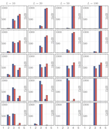
1 2 3 4 5 500 1000 12d B 500 1000 15d B 500 1000 18d B 500 1000 21d B 500 1000 24d B L = 10 1 2 3 4 5 500 1000 12d B 500 1000 15d B 500 1000 18d B 500 1000 21d B 500 1000 24d B L = 20 1 2 3 4 5 500 1000 12d B 500 1000 15d B 500 1000 18d B 500 1000 21d B 500 1000 24d B L = 50 1 2 3 4 5 500 1000 12d B 500 1000 15d B 500 1000 18d B 500 1000 21d B 500 1000 24d B L = 100
Fig. 2. Histograms of selected model orders ˆM for different SNR (top to bottom) and number of componentsL (left to right). The blue and red bars correspond to multiscale model selection strategies MV and RS, respectively (cf., Section 3.2). The ground truth isM = 4.
4.2. Model order selection performance
Fig. 2 plots the histograms of the model orders that are selected for the noisy mixtures of ofBm using the MV and RS procedures and (8) (blue and red bars), for various SNR values (increasing from bottom to top) and mixture dimensionsL (from left to right), respectively. The results lead to the following conclusions. First, the model order selection procedure is overall satisfactorily accurate as long as the SNR is sufficiently large. For instance, a large majority of decisions are correct for21dB SNR and L ≥ 20. Second, except for very severe SNR, the procedure does not detect more components than there actually are in the mixture, regardless of the SNR value andL. As a result, the decisions are slightly conservative (i.e., ˆM ≤ M ) on average. This can be heuristically interpreted as follows. For small SNR, the ofBm components with smallestHmare confounded with the noise, hence leading to underestimation ofM . By contrast, for large SNR, the gap between noise and ofBm components becomes large, leading to two distinct groups of eigenvalues and no ambiguity in the composition of the mixture.
Further, the MV and RS strategies for combining information from different scales lead to comparable results, with slightly bet-ter performance for RS; for instance, for18dB SNR and mixture dimension L = 50, RS yields 58% correct decisions, while MV underestimates the number of components in more than45 out of 100 cases. Finally, it is interesting to note that the performance of the proposed approach increases for large mixture dimensionL (“blessing of dimensionality”). Indeed, correct decisions are given with higher probability for largeL. Moreover, it is observed that for
0 5 10 15 20 25 0 0.02 0.04 0.06 0.08 0.1 0.12 SNR(dB) bias L=10 L=20 L=50 L=100 0 5 10 15 20 25 0 0.02 0.04 0.06 0.08 0.1 0.12 SNR(dB) std 0 5 10 15 20 25 0 0.02 0.04 0.06 0.08 0.1 0.12 SNR(dB) rmse
Fig. 3. Estimation performance for ofBm parameters fromM = 4 largest eigenvalues Λ(2j) for different L as a function of SNR: bias, standard deviations, and rmse (from left to right).
smallL, the estimates ˆM are spread out between different values, while for largeL, the procedure always tends to prefer one single value ˆM for a given SNR value.
4.3. Estimation performance
Fig. 3 reports results on the average estimation performance, evalu-ated over100 independent realizations, for the exponents Hm corre-sponding to theM = 4 largest eigenvalues Λ(2j) of Z, as a function of SNR and mixture dimensionL: bias (left), standard deviations (std, center) and root-mean squared errors (rmse, right); results are given as the square root of the averaged (over theM = 4 compo-nents) squares of the quantities and lead to the following comple-mentary conclusions. First, estimates ˆHmare also more accurate for largeL, which mirrors the results of Section 4.2: the standard de-viations of estimates forL = 10 are up to twice as large as those yielded forL = 100. This has never been reported before and in-dicates that the multivariate estimation procedure benefits from ex-tra robustness when the ofBm components are embedded in a high-dimensional (L ≫ M ) mixture (cf. [24] for a related analysis in a different context). Second, for a small SNR andL, estimation accu-racy is limited by biased estimates (because ofBm components are drowned in noise). Finally, for large SNR, estimation variances be-come independent of the noise level because they converge to the variance of ˆH for the noise-free case (essentially controlled by the effective sample size, i.e.,N , j1andj2).
5. CONCLUSIONS
In this work, we propose a method for estimating the number of mul-tivariate self-similar components (sources)M in L ≥ M noisy time series. The method relies on the ofBm model for multivariate self-similarity, on a multivariate estimation method for the Hurst eigen-valuesH of ofBm, and on the use of classical information theoretic criteria applied to the multiscale eigenstructure of the wavelet spec-tra of the noisy observations. To the best of our knowledge, this work reports for the first time i) that the estimation ofH when L > M based on multivariate procedures has satisfactory performance, and ii)an operational procedure for the estimation ofM in multivariate self-similarity with considerable accuracy, including in large dimen-sional situations. In the model selection procedure, wavelet spectra are combined across scales using averages or majority votes; alter-native strategies will be studied in future work; similarly, different model selection criteria could be employed, e.g., using more accu-rate models for the eigenvalue distributions - classical AIC was used to provide a proof of concept. In future work, the proposed tools will be used in the modeling of multivariate scale-free dynamics in data from macroscopic brain activity (M/EEG, fMRI).
6. REFERENCES
[1] P. Ciuciu, G. Varoquaux, P. Abry, S. Sadaghiani, and A. Klein-schmidt, “Scale-free and multifractal time dynamics of fMRI signals during rest and task,” Frontiers in physiology, vol. 3, 2012.
[2] N. Zilber, P. Ciuciu, P. Abry, and V. Van Wassenhove, “Mod-ulation of scale-free properties of brain activity in MEG,” in IEEE International Symposium on Biomedical Imaging (ISBI). IEEE, 2012, pp. 1531–1534.
[3] F. A. Isotta, C. Frei, V. Weilguni, M. Perˇcec Tadi´c, P. Lassegues, B. Rudolf, V. Pavan, C. Cacciamani, G. Antolini, S. M. Ratto, and M. Munari, “The climate of daily precipita-tion in the alps: development and analysis of a high-resoluprecipita-tion grid dataset from pan-alpine rain-gauge data,” International Journal of Climatology, vol. 34, no. 5, pp. 1657–1675, 2014. [4] D. Veitch and P. Abry, “A wavelet-based joint estimator of the
parameters of long-range dependence,” IEEE Transactions on Information Theory, vol. 45, no. 3, pp. 878–897, 1999. [5] H. Wendt, P. Abry, and S. Jaffard, “Bootstrap for empirical
multifractal analysis,” IEEE Signal Processing Magazine, vol. 24, no. 4, pp. 38–48, 2007.
[6] G. Samorodnitsky and M. Taqqu, Stable non-Gaussian random processes, Chapman and Hall, New York, 1994.
[7] B. B. Mandelbrot and J. W. van Ness, “Fractional Brownian motion, fractional noises and applications,” SIAM Reviews, vol. 10, pp. 422–437, 1968.
[8] M. Maejima and J. D. Mason, “Operator-self-similar stable processes,” Stochastic Processes and their Applications, vol. 54, no. 1, pp. 139–163, 1994.
[9] J. D. Mason and Y. Xiao, “Sample path properties of operator-self-similar Gaussian random fields,” Theory of Probability & Its Applications, vol. 46, no. 1, pp. 58–78, 2002.
[10] G. Didier and V. Pipiras, “Integral representations and proper-ties of operator fractional Brownian motions,” Bernoulli, vol. 17, no. 1, pp. 1–33, 2011.
[11] G. Didier and V. Pipiras, “Exponents, symmetry groups and classification of operator fractional Brownian motions,” Jour-nal of Theoretical Probability, vol. 25, pp. 353–395, 2012. [12] P. Abry and G. Didier, “Wavelet estimation for operator
frac-tional Brownian motion,” Bernoulli, vol. 24, no. 2, pp. 895– 928, 2018.
[13] P. Comon and C. Jutten, Handbook of Blind Source Separation: Independent Component Analysis and Applications, Academic Press, 2010.
[14] T. S¨oderstr¨om and P. Stoica, System identification, Prentice-Hall, Inc., 1988.
[15] P. Stoica and Y. Selen, “Model-order selection: a review of in-formation criterion rules,” IEEE Signal Processing Magazine, vol. 21, no. 4, pp. 36–47, 2004.
[16] A. P. Liavas and P. A. Regalia, “On the behavior of informa-tion theoretic criteria for model order selecinforma-tion,” IEEE Trans-actions on Signal Processing, vol. 49, no. 8, pp. 1689–1695, 2001.
[17] J. P. C. L. Da Costa, A. Thakre, F. Roemer, and M. Haardt, “Comparison of model order selection techniques for high-resolution parameter estimation algorithms,” in Proc. 54th
International Scientific Colloquium (IWK’09), Ilmenau, Ger-many, 2009.
[18] R. A. Johnson and D. W. Wichern, Applied multivariate statis-tical analysis, vol. 4, Prentice-Hall New Jersey, 2014. [19] P. Abry and G. Didier, “Wavelet eigenvalue regression for
n-variate operator fractional Brownian motion,” arXiv preprint arXiv:1708.03359, 2017.
[20] G. Didier, H. Helgason, and P. Abry, “Demixing multivariate-operator selfsimilar processes,” in IEEE International Confer-ence on Acoustics, Speech and Signal, Processing (ICASSP), Brisbane, Australia, 2015, pp. 1–5.
[21] P. Abry, G. Didier, and H. Li, “Two-step wavelet-based estima-tion for Gaussian mixed fracestima-tional processes,” arXiv preprint 1607.05167, 2018.
[22] P.-O. Amblard and J.-F. Coeurjolly, “Identification of the mul-tivariate fractional Brownian motion,” IEEE Transactions on Signal Processing, vol. 59, no. 11, pp. 5152–5168, 2011. [23] S. Mallat, A Wavelet Tour of Signal Processing, Academic
Press, San Diego, CA, 1998.
[24] C. Lam and Q. Yao, “Factor modeling for high-dimensional time series: inference for the number of factors,” The Annals of Statistics, vol. 40, no. 2, pp. 694–726, 2012.