Science Arts & Métiers (SAM)
is an open access repository that collects the work of Arts et Métiers Institute of
Technology researchers and makes it freely available over the web where possible.
This is an author-deposited version published in: https://sam.ensam.eu Handle ID: .http://hdl.handle.net/10985/18690
To cite this version :
Jacques VERDU, BRUNO FAYOLLE - Ageing and Durability of Organic Polymers - 2011
Any correspondence concerning this service should be sent to the repository Administrator : [email protected]
Chapter7
Ageing and durability
of organic polymers
Definitions. General comments 7.1.1. Ageing
“Ageing” is any slow and irreversible phenomenon (under usage conditions) of a material’s structure, morphology or composition, under the effects of its own instability and/or interaction with the environment.
Any condition is considered to be slow when the kinetics are not apprehensible in a time scale which is compatible with economic restraints.
The classic approach of predicting long-term behavior consists of carrying out accelerated tests simulating, as accurately as possible, natural ageing and to presume that the hierarchy of stability for several materials is the same in accelerated and natural ageing. The modern approach consists of developing a kinetic model derived from analyzing degradation materials. Accelerated ageing is, then, used to identify the model parameters.
7.1.2. Lifetime
The lifetime (tF) is specific to a property (P) of the material, as crucial as possible
for the application considered, and for which it is possible to define a critical value Pf.
kinetic model must allow the following function to be established: P = f(t), which describes the evolution of P over the ageing process. The lifetime is then defined by:
) P ( f tF 1 F
where f-1 is the reciprocal function of f. P
F is often called the end-of-life criterion.
7.1.3. Extrapolation principle
The classic approach consists of considering that the simple laws established for basic processes also apply to complex processes, such as ageing. For example, in thermal ageing (a rise in temperature leading to acceleration), we can write:
RT E exp t tF F0 (Arrhenius law)
The tests accelerated at different temperatures enable us to identify tF0 and E. Next,
it is then sufficient to extrapolate to use temperature to obtain lifetime.
In the case of ageing by irradiation (photo or radiochemical), it may be useful to consider that the end-of-life is an isodose state, in other words:
Fu u Fa at d t d where
d is the dose rate (light intensity for photochemical ageing), indices a and u are specific to accelerated and natural ageing, respectively.
In fact, neither of the two laws above can be considered as being systematically valid for ageing. Using these laws without control may lead to important errors of appreciation.
For kinetic approaches, the ageing mechanism is divided into elementary processes. For each of these processes, the laws mentioned above are applicable, when reformulated in terms of elementary rates:
et v Gd RT E exp v v j i 0 i i
The global kinetic function P = f(t) includes all the associated elementary kinetic parameters in a more or less complex mathematical equation. Extrapolation under natural ageing conditions will be achieved by extrapolating all the elementary parameters by their associated law.
Let us use a simple example from thermal ageing where the total rate is the sum of the rates of two elementary processes which obey the Arrhenius law:
RT H exp v RT H exp v v 0a a 0b b
The elementary process rates are equal at temperature TC,such as:
a 0 b 0 a b c v v Ln . R H H T
Away from Tc, one of the processes is insignificant in relation to the other, and the
Arrhenius law may be an acceptable estimation to calculate v:
RT H exp v v 0i i with i = a or b.
On the other hand, around temperature Tc, v does not obey the Arrhenius law at
all. In this domain, lifetime predictions bypass the identification of the parameters which characterize the elementary processes v0a, Ha, v0b, Hb and the calculation of the
sum of the two Arrhenius terms.
In practice, cases when the total rate of a process results from the sum of elementary rates are not rare.
7.1.4. Induction period
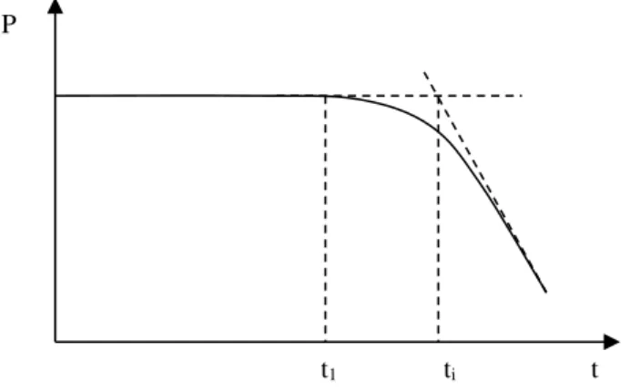
In many cases, ageing kinetics are characterized by the existence of an initial period during which there is no noticeable evolution of the polymer usage properties (Figure 7.1).
Generally, an induction period is a period of time over which the material preserves its original properties. There are three main reasons which explain such behavior (largely non-linear behavior, it must be said):
– induction phenomenon is specific to the chemical reaction responsible for ageing. Oxidation processes (radical reactions in branched chains) often manifest this characteristic at low temperatures (typically when T 150°C);
– induction phenomenon is related to the presence of an efficient stabilizer. So long as this stabilizer is not completely consumed, degradation remains insignificant;
– the chemical structure evolves under an ageing effect, but the considered properties only evolve beyond one threshold. Embrittlement phenomena often manifest this characteristic.
Figure 7.1.Diagram representing kinetics of the evolution of usage property P with an induction period of length ti
Obviously the combination of two or three causes above is not excluded.
Figure 7.1 enables us to understand the remote amount of interest, so as not to say the uselessness, in punctual tests based on the study of one ageing duration length. For example, a duration test where t1 < ti lets us establish that ti is higher than the test
time, but we cannot be sure, however, if t1 = 0.95 ti or 0.1 ti or 0.01 ti.
t ti
t1
In conclusion, any analysis relevant to ageing bypasses the stage where the kinetic curves of the material’s evolution are established in unique time scales which allow for a significant evolution, if possible to a state where it would then be considered unsuitable for the characterized usage.
7.1.5. Different types of ageing
7.1.5.1. Chemical ageing
Ageing induced by a chemical modification of the material’s structure.
7.1.5.2. Physical ageing
Ageing affecting chain conformation, morphology or the material composition without changing the chemical structure of the macromolecules.
7.1.5.3. Thermal ageing
Ageing where the kinetics only depend on temperature and atmospheric composition. This can be either physical, chemical or both.
7.1.5.4. Wet ageing
Ageing induced by the interaction of the material with water present in the environment, either as a liquid or vapor. This interaction can be either physical or chemical.
7.1.5.5. Photochemical ageing
Chemical ageing induced by the interaction of a polymer with light rays (generally solar UV radiation), where oxygen from the atmosphere generally plays a large role (photo-oxidation).
7.1.5.6. Radiochemical ageing
Chemical ageing induced by the interaction of a polymer with ionizing rays neutrons, etc.), where oxygen from the atmosphere may play a large role, especially at low dose rates.
7.1.5.7. Biochemical ageing
Chemical ageing induced by the interaction of a polymer with living organisms (bacteria, moulds, etc.).
7.2 Physical ageing
7.2.1. Physical ageing by structural relaxation (broad meaning)
The two phenomena responsible for the solidification of polymers at the end of their processing operations are vitrification and crystallization. Both of which are kinetic phenomena which lead to a thermodynamic state out of equilibrium. Glasses have an excess of unstable conformations and free volume (section 5.2.5). Semi-crystalline polymers are not completely crystallized; their melting point is clearly lower (often by a few tens of degrees) than its equilibrium value.
If, in their use conditions, a residual molecular mobility takes place in these polymers (β movements in glass, movements in the rubbery amorphous phase of semi-crystallines), then they will slowly move towards an equilibrium (structural relaxation).
The general characteristics of this type of ageing (wrongly called “physical” ageing because there are other physical mechanisms of ageing) are the following:
– ageing results in a compacification of the matrices and a loss of enthalpy; – the stress at the plastic yield increases;
– the creep compliance decreases;
– evolution slows down but may continue over recorded time.
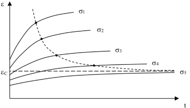
The evolution of creep compliance J(t) has been the subject of quantitative studies, particularly by Struik [STU 78] for organic glass.
The creep curves of samples aged during tv, 10tv, 100tv, etc., take the shape seen
in Figure 7.2. If we say that v 2 v 1 v t t Log
a is the logarithm of the ageing time ratio, and
fl 2 fl 1 fl t t Log
a the corresponding interval of the creep curves on the logarithmic time
scale, we observe that 1 a a
fl v .
In other words, increasing the ageing time by a decade causes an increase in the characteristic creep time by approximately a decade.
This is a very general property of structural relaxation ageing, whether it is a question of polymers, molecular organic materials (glucose), sand heaps or emulsions.
Figure 7.2.Creep curve (in a log – log scale), of aged samples TV, 10tv and 100tv at a temperature lower than Tg
The reduction in creep compliance, as with the stress increase at the plastic yield, would be an advantage in many applications. Unfortunately, it is compensated by an important reduction in ductility/toughness (Figure 7.3a).
Increasing yield stress (up to 20 MPa for a polymer such as polycarbonate), the loss of ductility without altering the molar mass distribution, and the appearance of an endotherm in the immediate vicinity of Tg (Figure 7.3b) allows us to recognize
structural relaxation ageing from another type of ageing, in the case of an amorphous glassy polymer.
1 10 100
Log J(t) tv 10 tv 100 tv
t (creep) Log tf
Figure 7.3. a) Shape of stress-strain curves from a new sample (o) and from a sample subjected
to ageing under structural relaxation (v).b) shape of (DSC) thermograms from a new sample (o) and from a sample subjected to ageing under structural relaxation (v)
7.2.2. Ageing by solvent absorption
Solvents plasticize polymers and therefore lead to a reduction in Tg and a reduction
in the yield stress in a ductile system.
However the most important effects, in practice, appear when the polymer is subjected to static stress.
Indeed, plasticization favors damage, in particular by crazing.
For example, let us consider a creep test where damage is detected by an optical method.
The behavior is represented by Figure 7.4.
Tg T Cp (v) (o) (v) (o) (a) (b)
Figure 7.4.Shape of the creep curves in the presence of a solvent. 1 >2 >3… etc. The black points represent onset of damage.The envelope of the points has a horizontal asymptote
at =C
We can see that there is a critical strain C, below which the material will not be
damaged. Value C is according to the polymer/solvent pair.
In simple cases (only slightly polar polymers, such as Polyphenyleneoxide (PPO), C varies with the solvent’s solubility parameter, according to Figure 7.5.
We must remember that certain vapors (H2O, CO2) are very important. In addition,
the plasticizers themselves can migrate from one polymer into the other and induce damage under stress.
Where complex parts are concerned, localized damage in the presence of solvent vapors may reveal the presence of residual stresses.
C t C S p
(2)
(1) l
L
Figure 7.5.Shape of the critical strain variation C with the solvent’s solubility parameter in the case of PPO. The curve’s minimum corresponds to S =p (the polymer’s solubility parameter).(○):crazes.(●):open cracks.The hatched area relates to the C values observed in the air.NB For polar polymers (PMMA for instance), the behavior is more complex, the curve C = f(S) may include several minima.
Solvent penetration in a polymer results in swelling, which can also generate strains related to differential. Damage problems induced by water diffusion in organic matrix composites have been, and are still, the subject of active research, particularly in aeronautics.
7.2.3. Ageing by additive migration
Thermodynamically, a polymer + additive mix is out of equilibrium. Since the additive’s concentration in the surrounding environment is nul, there is no equality in its chemical potential within the environment and the polymer.
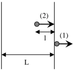
To restore this equality and move towards equilibrium, the additive tends to migrate out of the polymer. This migration is made up of two stages (Figure 7.6).
The first stage is the movement into the environment for the molecules close to the surface, in other words, crossing over into the polymer/environment interface. In gaseous environments, (e.g., the atmosphere), the evaporation of the additive is responsible for this stage. In liquid environments, the additive’s dissolution by the said liquid plays the same role. Let us note that a second polymer, in contact with the first, may play the same role as a liquid. Polymers also have a tendency to switch stabilizers. Plasticizers (PVC, for example) are well-known for their tendency to migrate into all sorts of polymers.
Figure 7.6.Diagram representing the two stages of a polymer’s migration outside a polymer
The second stage begins as soon the first molecules of the additive which leave during the first stage have created a concentration gradient. This is the “motor” of the molecular diffusion occurring in the core towards the surface. Duration td of the
molecule’s path of length l is given, in the case of diffusion which obeys the Fick law by:
We can see that td rapidly increases with the sample’s thickness L.
Therefore, we can now distinguish two kinetic regimes.
7.2.3.1. Mode controlled by evaporation (or dissolution)
When L is low (fibers, films) and diffusivity D is high enough, evaporation is slower than diffusion and therefore controls the migration’s total kinetics.
Thus, concentration C of the additive in the polymer decreases in an exponential way with time:
HC dt
dC
The evaporation rate constant H decreases with the additive molar mass and its cohesive energy density.
7.2.3.2. Mode controlled by additive diffusion
When L is high and D is low, diffusion controls kinetics. In the simplest of cases, the Fick law is applied:
2 2 x m D t m
(m = mass variation related to additive loss)
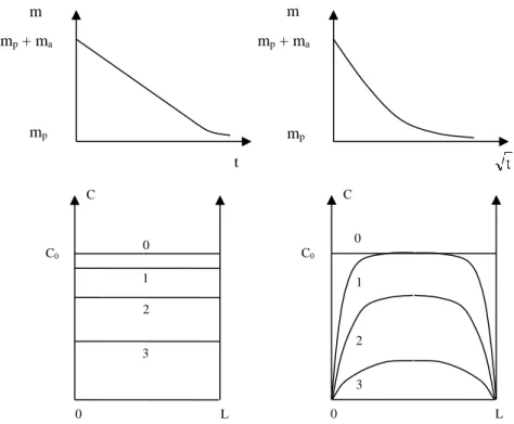
In the initial time period, the mass decreases in proportion to the square root of the time. A concentration gradient is established in the thickness of the sample (Figure 7.7). D l t 2 d
Figure 7.7.Migration controlled by evaporation (left) and by diffusion (right). Top: shape of the kinetic curves of mass evolution. mp + ma = polymer mass + additive mass (mp = polymer mass). Bottom: additive concentration profile in the sample’s thickness at different times: 0 < t1 < t2 < t3 < t4.
When the additives have relatively high molar masses, their evaporation (or generally, their cross over from the polymer/environment interface) is slow. Their concentration at the surface is thus intermediate between the initial concentration C0
and 0. This boundary condition must be taken into account to solve the diffusion equation.
When the additives are strongly concentrated (e.g. plasticizers) they change matrix properties, and their diffusivity then becomes a function of their concentration (D increases with C). There are some complications which may arise when the additive’s migration is accompanied by a phase transition, for example, in the case of plasticized PVC we may expect the profile seen in Figure 7.8.
0 L 0 C 3 2 1 C0 C0 L 0 0 1 2 3 C t mp + ma m mp mp + ma m mp
Figure 7.8.Presumed shape of the concentration profile in the plasticizer (mass fraction) and the local glass transition temperature in a plasticized PVC sample subjected to ageing at
room temperature
We can see, however, that in the central area, the polymer has retained a rubbery state. On the other hand, in a superficial layer of thickness la, the polymer is glassy.
As the diffusion coefficient varies from at least one order of magnitude at glass transition, the real profile will be more likely to take the shape seen in Figure 7.9.
In such cases, the diffusion front is very abrupt and the mass variation is a linear time function.
In terms of usage properties, a loss of additives may result in the loss of properties that they were supposed to bring originally: long term resistance for stabilizers, flexibility for plasticizers, etc. When the additives are initially strongly concentrated (plasticizers), their loss leads to volume shrinkage (mass loss). The volume shrinkage may generate strains and lead to crack growth.
C L 0 0 1 2 3 4 C (%) L 0 30 20 10 0 Tg (°C) 80 40 0 -40 -80 -120 la L-la
Figure 7.9.Real shape of the concentration profile in plasticization, in the example illustrated by Figure 7.7, at times 0 < t1 < t2 < t3 < t4
7.3 Chemical ageing - general aspects
7.3.1. The two large families of chemical ageing processes
It is important to distinguish the processes which only affect lateral groups, without changes to the macromolecular skeleton, from processes which alter the macromolecular skeleton. Indeed, the first processes do not affect mechanical behavior (at reasonable conversion ratio), whereas the second processes greatly affect the mechanical behavior, even at low conversion ratio.
7.3.1.1. Processes affecting lateral groups
Halogenation and sulfonation processes etc., are likely to replace various hydrogen groups carried in the chain by chlorine atoms, SO3 groups ect…, but such processes
are rarely encountered in an ageing context. In contrast, oxidation processes are very frequent. These processes also affect the macromolecular skeleton, but for now we will only deal with the consequences of altering lateral groups, e.g.:
CH2 CH OH or CH OOH or C O
A hydrocarbon group, only slightly polar, is transformed into an oxygenated polar group (ketone), or even a very polar group (alcohol). If this transformation occurs in a matrix which is initially rich in polar groups, there will be few consequences on the physical properties. On the other hand, if it occurs in a matrix which is only slightly polar (polyolefin, hydrocarbon elastomers), then resultant changes in polarity may have significant consequences on all the physical properties linked to this characteristic, particularly dielectric permittivity, refraction index, surface energy, and wettability.
Some processes lead to the formation of colored species. In the case of PVC, such as sequential elimination of hydrogen chloride:
CH2 CH2Cl CH2 CH2Cl CH2 CH2Cl
HCl +
Sequences of more than five to seven conjugated double bonds absorb in the visible spectrum and absorption spreads towards large wavelengths when the number of conjugated double bonds increases. The material will appear yellow-brown or purple according to the distribution of the conjugated sequence lengths. These species have very high molar extinction coefficients, up to more than 105 l.mol-1cm-1. The
coloring appears at low, or even very low, conversion ratio.
In polymers made up of aromatic nuclei, their oxidation leads to quinoid species which absorb near UV and violet. These materials (polystyrene, polycarbonate, PET, polyesters cross-linked by styrene, epoxides, etc.) undergo a degree of yellowing over ageing.
The oxidation of saturated polymers (PE, PP, for example) may also lead to colored species if the material initially contains traces of metallic impurities which can potentially form colored complexes with some oxidation products, such as carbonyls.
Lastly, some stabilization processes, particularly with aromatic amines or phenols, are also likely to create strongly colored species which can be distinguished from the species already present on the polymers, by the fact that they can be extracted by solvents.
7.3.1.2. Macromolecular skeleton modification process
Two types of processes can be distinguished here (Figure 7.10).
Random chain scission
Random chain welding (crosslinking)
Figure 7.10.Diagram representing two types of macromolecular skeleton modification processes
Of course, the two process types can coexist. If s and x are the respective numbers (moles) of scission and crosslinking events per mass unit, the average molar mass in number Mn (initial value Mn0) variation and weight (initial value Mw0) is given by the
following system of equation:
x 2 2 s M 1 M 1 x s M 1 M 1 0 w w 0 n n
We are able to see that if s > 4x, chain scission prevails.
On the other hand, if s < 4x, crosslinking will prevail.
So long as the material stays 100% soluble, then this system of equations enables us to determine s and x from average molar masses Mn and Mw. But if crosslinking
prevails, the material bypasses the gelation point and an insoluble fraction appears. We can then apply the Charlesby theory:
x M 1 x 2 s w w 0 w 2 1 s s
where ws is the soluble fraction.
This equation is easy to exploit if s and x vary in a linear way with time, which is generally the case in radiochemical ageing at relatively high dose rates.
7.3.1.2.1 Consequences of chain scission
As seen in Chapter 5 (section 5.2.5), fracture properties of a linear polymer vary enormously around a critical molar mass MC’. We can then expect that the fracture
properties of an initially ductile/tough polymer, drop significantly when its molar mass reaches value MC’. Let us consider a chain scission process at constant rate v:
In the absence of crosslinking: Therefore: t vM 1 1 M M 0 n 0 n n
Let us consider an example where Mn0 = 100 kg.mol-1, v = 10-4 mol.kg.j-1 and MC’ =
20 kg.mol-1. The evolution of M
n and the ultimate elongation are represented in Figure
7.11.
These results call for the following remarks:
– where the chain scission reaction occurs at constant rate, the molar mass varies hyperbolically;
– Mn varies monotonously whereas the ultimate elongation drops catastrophically
when Mn = MC’;
– embrittlement occurs when the number of chain scissions is: 04 , 0 M 1 ' M 1 s 0 n C c mol.kg-1 0 n n M 1 M 1 s
Figure 7.11.Variation in the number average molar mass Mn, and of the relative ultimate elongation r/r0 in a polymer subjected to ageing by random chain scission at a rate of 10-4
moles scissions per kg per day
As an example, in a polymer such as polyamide 11 or PET, the concentration in monomer units is 5 mol.kg-1. In other words, embrittlement occurs at a very low
conversion ratio, which is sometimes difficult or impossible to detect by spectrochemical means. The elastic and yielding properties are practically unaffected at such conversion ratio. We understand, then, that embrittlement caused by ageing is an important aspect of research. Whatever the importance of other usage properties, no application can tolerate the geometric integrity of the samples being damaged by crack growth.
In some cases of superficial ageing, localized embrittlement may create a network of microcracks without a notable influence on the total fracture behavior. However, microcracking will change the appearance of the surface which may also have an economic impact in applications where questions of aesthetics are important.
In networks (vulcanized elastomers, thermosets), random chain scission can destroy chains which are elastically active. Typically, at low conversion ratio, for a quasi ideal network:
0 20 40 60 80 100 120 0 200 400 600 Temps (jours) M n ( k g .m o l -1 ) 0 0,2 0,4 0,6 0,8 1 R/ R0 Time (days)
ν = ν0 – s
where ν and ν0 are the concentrations in elastically active chains, before and after
ageing respectively, and s is the number of chain cuts. Let us remember that v can be determined by measurements of the elasticity modulus in rubbery state:
RT G (G: shear modulus) therefore:
G G
RT 1 s 0 Chain cuts can decrease the elastomer’s modulus. On the other hand, they do not directly influence the thermosets modulus in glassy state.
Fracture properties tend to drop catastrophically, but the structure/property relationships are still relatively unknown in this domain.
7.3.1.2.2 Crosslinking consequences
For exclusive crosslinking (no chain scission), Mw and Mn increase, the
polymolecularity index p = Mw/Mn also increases, p and Mw diverge at the gelation
point which corresponds to:
0 w g M 2 1 x
Here, we also see that gelation relates to a very weak conversion ratio. Two active sites are needed to make a crosslink, therefore the transformation rate at gelation point
is 0 w g M 1
y . In polyethylene, for example, for Mw0 = 100 kg.mol-1 we would obtain
that yg = 10-2 mol.kg-1 whereas the concentration in potentially reactive sites (-CH2-)
is approximately 7,000 times greater. Of course, certain properties, particularly flow properties in molten state, change well before the gelation point. In particular, viscosity in molten state rapidly increases and the Newtonian plateau tends to disappear.
Elongation at break gradually decreases, whereas the stress at break increases, at least in an elastomer’s initial ageing phase. Where thermosets are concerned, we know that Tg increases and that the ductility tends to decrease.
7.3.2. Diffusional phenomena in chemical ageing
Oxidation and hydrolysis (two frequent modes in chemical ageing) involve penetrating a small reactive molecule (O2, H2O) from the environment in the material.
We can define two characteristic times – one being diffusion, the other a chemical reaction – for a simplified approach to the problem:
− in the case of diffusion, characteristic time can be defined by: D
L t
2
D where L is the sample’s thickness and D the diffusion coefficient of the
molecular reactant;
− in the case of the reaction, we can use the following definition:
C R
v C
t where C is the equilibrium concentration of the reactant in the polymer, and vc is the rate of the reactant consumption by the reaction in the sample’s
superficial layer where the reactant’s concentration is effectively C. The equality of the two times is achieved for:
tD = tR meaning that 2 / 1 C C v DC L
– if the sample’s thickness is L << LC, then diffusion is quick enough in relation to
the reaction, in order to saturate the sample in its entire volume at any time;
– if the sample’s thickness is L >> LC, then any molecular reactant is consumed in
a layer with a thickness of the order of LC and the sample’s core is not degraded.
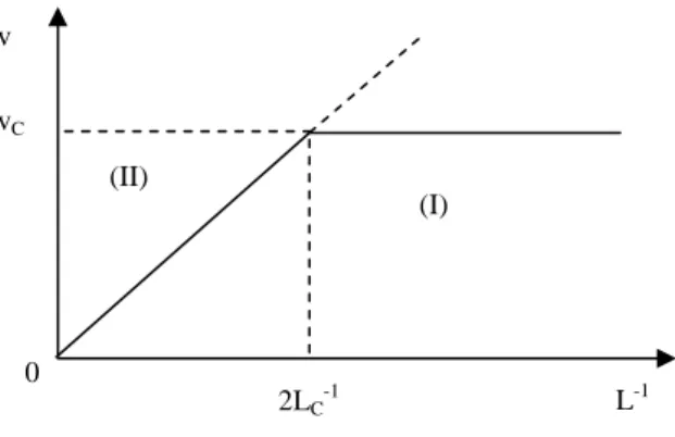
By comparing the total degradation rates of samples which differ in thickness, we can build the graph in Figure 7.12 which enables us to determine LC.
Figure 7.12.Shape of degradation rate variations with the reverse of the sample’s thickness
Two regimes can be distinguished: the regime which is not controlled by diffusion (I) where the (total) degradation rate is independent of the thickness, and the regime which is controlled by diffusion (II) where the (total) degradation rate is in proportion to the reverse thickness since the thickness of the degraded layer (LC) is independent
of the whole sample thickness. The boundary value is 2LC if the molecular reactant
penetration is carried out by the two sides of the sample, which is often the case.
For a more rigorous and detailed approach to the problem, the relationship vC =
v(C) expressing the reactant’s consumption rate according to its concentration in the case of a homogeneous reaction (L<<LC) must be established. The variation rate of
the reactant’s local concentration is, then, given by the equation:
2 2 x C D ) C ( v t C
where x is the spatial coordinate (in the direction perpendicular to the sample’s surface) and D is the molecular reactant’s diffusion coefficient.
Many authors assume rapid installation of a stationary state such as:
) C ( v x C therefore 0 t C 2 2
Therefore, we assume that the molecular reactant has a stationary concentration profile in the sample: C = f(x), which is a result of solving the above differential equation. v vC 0 2LC -1 L-1 (II) (I)
In hydrolysis processes, for example, we can generally say that:
vC = KC (pseudo first order process)
In oxidation processes, vC varies with C according to a pseudo-hyperbolic curve
which can be approximate by:
C 1 C vC
where α and β are parameters which can be clarified according to the rate constants of elementary processes which are constitutive of the radical oxidation chain reaction.
Numerical solutions of kinetic equations and reaction-diffusion coupling equations free us from simplifying hypotheses, particularly those of a stationary state which is often difficult to justify.
Let us return to the scaling relationship of the simplified approach to the problem:
2 / 1 C C v DC L
C generally hardly varies with temperature.
D generally obeys the Arrhenius law: RT E exp D D 0 D
For vC, we may also consider the Arrhenius law to be obeyed in a first approach:
RT E exp v vC C0 C .
We can see that LC should also obey the Arrhenius law:
) E E ( 2 1 E with RT E exp L LC C0 L L D C
With regard to thermal ageing, we generally have EC > ED, so that LC is a
decreasing function of temperature (Figure 7.13).
Figure 7.13.Diagram representing degradation profiles (thermo-oxidation) at two different temperatures: T1 < T2 and at a sensitively equal total degradation rate
In the case of ageing by irradiation, D and C are independent of radiation intensity I, whereas vC can be approximately obtained by vC I . It results that
2 / C I
L
LC decreases slowly with I because α is generally lower than unity (α = ½ in the
simplest models).
The fact that the thickness of the degraded layer is generally a decreasing function of the “aggressiveness” of the exposure conditions may go against intuition, but it is a fact which has been checked many times.
7.3.2.1. Consequences of superficial deterioration on usage properties
Of course, surface properties (color, wettability, etc) are not dependant on the degradation gradients. On the other hand, these gradients may play an important role in terms of mechanics.
Schematically, a polymer sample (initially ductile/tough and homogeneous) is gradually transformed into two layers by ageing. The inner layer remains ductile/tough, but the superficial layer is brittle and cracks easily. A crack which starts in the superficial layer will quickly make its way into the superficial/inner layer
v
x T2
T1
interface. It will either be blunted, or it will propagate, leading to a break in the sample (Figure 7.14).
Figure 7.14. Diagram representing possible crack growth modes of a sample subjected to surface level ageing. The dots symbolize degradation: I is the initial sample, II is the aged sample before the embrittlement threshold, III is the sample which is close to the embrittlement threshold, IVa is a sample with blunted crack, with the crack making its way to the degraded/non-degraded interface, IVb shows the crack crossing the degradation front, Va and Vb show the progression of the degradation front at the top of the crack.
As a first approach, we may consider that the weakened superficial layer is equivalent to a notch of the same depth. Fracture mechanics (Griffith 1921) enable us to predict that there is a critical notch depth, which will not initiate crack growth if it is not reached. This critical depth depends on the material’s strength, which depends on crack propagation rate.
Therefore we expect that a very rapid ageing process, leading to a low level of thickness of the oxidized layer, changes fracture behavior comparatively less than a slower ageing process. This has been checked many times in experiments.
7.3.3. Towards a non-empirical lifetime prediction
Ageing is a complex phenomenon but which can be broken down into elementary mechanisms which obey simple kinetic laws (Arrhenius law, proportionality of rate to light intensity, etc.). However, the “target” of chemical ageing is the molecular scale structure, but the usage properties depend on higher scale structures [AUD 07]. Moving away from these reports, we can develop a strategy for predicting non-empirical lifetimes, represented in the following diagram (Figure 7.15).
(IVa) (Va)
(IVb) (VIa)
(III) (II)
Figure 7.15.Diagram illustrating the strategy for predicting non-empirical lifetime
Vector A represents a chemical kinetics model, showing the evolution of the material to the molecular scale. Vector B symbolizes the path from the molecular scale to the macromolecular scale. This process involves knowledge of the elementary event of scission/crosslinking, and reaction statistics. Vector C represents reaction-diffusion coupling. All the other vectors show relationships coming from polymer physics.
For different reasons (mechanism hyper-complexity, gaps in polymer physics, etc.) some of the relationships involved in this diagram cannot be translated in mathematical terms. On the other hand, achieving all the procedure steps in a non-empirical way may constitute an unrealistic research program from an economical point of view. It will be, then, a matter of injecting a minimum of empiricism into the model so that it works, but by making the conducted hypotheses as clear as possible.
From this, the chosen strategy seems to be the best possible compromise between the need for scientific rigor, which guarantees the reliability of the prediction, and economic constraints.
B
Structure at molecular scaleStructure at macromolecular scale
Structure at macroscopic scale (skin-core) Use properties Time
0
t
S
0S
tM
0M
tQ
0Q
tP
0P
tA
C
7.3.4. Oxidation - general aspects
For the majority of practical cases in thermal, photochemical or radiochemical ageing, the main cause for ageing is oxidation of the polymer by interaction with oxygen in the atmosphere.
In all cases oxidation results from radical chain reactions and the kinds of ageing mentioned above, they only differ by initiation (in mechanistic terms)
The standard mechanistic scheme, drawn up by an English team in the 1940s [BOLL 46], is the following:
(I) polymer (PH) P° (ri) (Initiation)
(II) P° + O2 PO2° (k2) (Propagation)
(III) PO2° + PH Per + P° (k3) (Propagation)
(IV) P° + P° Inactive products (k4) (Termination)
(V) P° + PO2° Inactive products (k5) (Termination)
(VI) PO2° + PO2° Inactive products (k5) (Termination)
As we have seen, initiation may be thermal, photochemical or radiochemical. It can be the result of a reaction which directly involves a non-degraded part of the polymer (radiochemical) or a reaction product, particularly a peroxide or hydroperoxide (Per).
Propagation involves two chemical processes, the second one (III) regenerating radical P° involved in the first one (II). Adding O2 to the radicals (II) is very fast (k2
~ 108 à 109 L.mol-1.s-1). The reaction between peroxyl radicals (PO
2°) and the polymer
is much slower (k3 ~ 0.01 to 10 L.mol-1.s-1, typical values at room temperature). PO2°
radicals can act abstracting hydrogen or adding to double bonds. In the first case, the product Per is a hydroperoxide (POOH). In the second, it is a peroxide (POOP).
The terminations (when there are no stabilizers) are bimolecular. Two radicals are deactivated mutually. We have, then:
k4 > k5 >> k6
When there is excess oxygen (low thickness sample, high O2 pressure, low
initiation rates), radicals P° are quickly transformed into PO2° by reaction II. The
probability of their reacting by other means becomes very low, and the scheme is simplified as follows in the case of propagation by hydrogen abstraction, for example:
(III) PO2° + PH + O2 PO2H + PO2° (k3)
(VI) PO2° + PO2° Inactive products + O2 (k5)
We can therefore distinguish two important cares:
Reaction (I) is carried out at constant rate ri (radiochemical initiation). Therefore,
a stationary state is quickly established, and the oxidation products gather at constant rate (figure 7.16).
We can easily show that products from initiation and termination are formed at a rate which is proportional to ri. On the other hand, hydroperoxide (propagation
product) is formed at rate
2 / 1 6 i 3 k 2 r ] PH [ k ) POOH ( v (proportional to r ). i
Oxygen is absorbed at rate:
2 / 1 6 i 3 i k 0 k 2 r ] PH [ k 2 r v .
Reaction (I) is the decomposition of peroxides or hydroperoxides formed during propagation. Initiation can be written as:
POOH α P° + β PO2° with if = 1, α = 2 and β = 0
if = 2, α = 1 and β = 1
When = 2 (more common at temperatures higher than 150°C), the kinetics are comprised of an induction period followed by a strong auto-acceleration preceding a steady state (Figure 7.16).
This type of reaction can be called a “closed loop” reaction because it produces its own initiator: hydroperoxide.
The kinetic analysis of the two process types show that kinetic behavior depends, in both cases, on two main factors: one which is extrinsic (relating to factors which are external to the polymer’s structure), for instance the initiation rate constant ki or
initiation rate ri which depend of radiation intensity in photo or radiochemical ageing.
The other factor is intrinsic e.g. only dependent of polymer structure, for instance the
ratio
6 3
k k
Figure 7.16. Shape of the kinetic curves of oxidation (a) for constant rate initiation (radiochemical ageing) (b) initiation by bimolecular decomposition ( = 2) of hydroperoxides (thermal ageing). In cases of unimolecular initiation ( = 1)of hydroperoxide (c) initial auto-acceleration is more progressive (some cases of photochemical ageing).
For “closed loop” processes, where [POOH]0 and [POOH] are the initial and steady
state hydroperoxide concentrations respectively, the ratio
0 POOH POOH ] [ ] [ determine the
amplitude of the auto-acceleration effects.
Polymers which do not contain CH bonds (polytetrafluorethylyene) or polymers only containing aromatic CH (PEEK, poly(ether sulfones), polyimides, etc.) are generally stable under oxidation. Polymers only containing methyls (polydimethylsiloxane) or methyls and methylenes (poly(methyl methylacrylate), polycarbonate, polyethylene) are moderately stable. Polymers containing tertiary CH (polypropylene), CH in α of heteroatoms (polyoxymethylene) or allylic CH (polydienic elastomers) are relatively instable. Let us note that it is a matter of a comparison of relatively little practical use because another (physical) factor plays an important role: oxygen diffusivity. The diffusivity is notably higher in elastomers than in glassy polymers. In other words, with equal reactivity, these latter will seem more stable because the thickness of their oxidized superficial layer will be lower.
Another potentially important factor: the property sensitivity to chemical acts of oxidation. For example, polypropylene becomes brittle in a number of chain scissions which are about 10 times smaller than for an amorphous polymer. According to mechanical criteria, it will seem 10 times less stable than an amorphous polymer with the same reactivity.
Despite these reservations, the classification of groups according to the following decreasing order of stability is completely valid:
(a)
t Qox
(b) (c)
ArH > -CH3 > -CH2-CH2-CH2- > -CH- -O-CH2 ~ =N-CH2- > -CH2-CH=CH-
CH3
7.3.5. Stabilization
Chain reactions, like radical oxidation, particularly when they produce their own intiation, have a major disadvantage in terms of practice: small problems may lead to big effects, in light of the strong auto-accelerating character of these reactions. But this disadvantage turns into an advantage when we plan to produce stabilization by additives (antioxidants). Indeed, since the reaction starts slowly and auto-accelerates, a small quantity of the stabilizers when adequately chosen may be enough to efficiently inhibit the process, a possibility which does not exist for step by step reactions, such as hydrolysis for example.
It generally seems difficult to change the propagation process. Yet, we can slow down initiation, for example, with stabilizers which destroy the hydroperoxides by non-radical means (sulfurs, phosphites). Or we can accelerate termination with stabilizers capable of capturing radicals P° or PO2° (phenols, aromatic amines,
hindered amines, nitroxyl radicals, etc.) In polyolefins, we may reach an efficient stabilization with stabilizing mass fractions lower than 0.5%. In polydienic elastomers, stabilizers can be used in concentrations higher than 1%. The most common appreciation method of stabilizer efficiency consists of determining the induction time at high temperatures (Figure 7.17).
Figure 7.17.Shape of thermograms at 190oC (raise in temperature under nitrogen, oxygen is admitted in the cell when the thermal equilibrium has been reached): a non-stabilized polyethylene (0), the same polyethylene stabilized by 0.3% of a phenol-phosphite combination.
It is important to note that the effectiveness of stabilizers also depends on physical factors, in particular: t (hours) 0 1 2 3 4 H 0 v
− solubility in the polymer. If the solubility level is low, the concentration level necessary for good levels of stabilization may not be reached. We may note that many stabilizers are comprised of long alkyl chains for instance in distearylthiodipropionate:
Thermal antioxidant hydroperoxide decomposor;
C O C8H17
O HO
UV absorber;
−diffusivity in the polymer. If the diffusivity level is too high, stabilizer loss through migration might decrease its efficiency. To reduce diffusivity, we can increase the molar mass (alkyl chain grafting, polymer stabilizers, etc.).
In addition to these significant factors, the choice of stabilizer must take other characteristics into account, such as:
− compatibility with the considered use (color, smell, toxicity, etc.);
− interaction with the environment. For example, phenolic stabilizers create highly colored species in the presence of nitrogen oxides; some hindered amines react with certain biocides used in farming, etc.;
− interaction with other polymer additives. For example, organic sulfides are not compatible with metals because they create highly colored metal sulfides.
Not all interactions are problematic, some stabilizers have an increased level of efficiency when combined with another additive. We can call this a secondary stabilizer. This is the case for combination of zinc and calcium soaps in PVC. Synergy mechanisms are very varied. In phenol-hydroperoxide decomposer systems, synergy is essentially the result of a kinetic effect due to the fact that each stabilizer exerts a favorable strain on a different step of the oxidation chain reaction. For Ca/Zn soaps in PVC, the “primary” stabilizer is the zinc soap, but the PVC-Zn reaction generates zinc chloride which is a powerful catalyst for the degradation of PVC. The role of Ca soap
is to eliminate zinc chloride by a double decomposition reaction which generates Zn soap.
7.4 Thermochemical ageing 7.4.1 Intrinsic thermal stability
In the absence of oxygen, polymers will decompose through their own instability, with this being controlled by thermochemical factors. Generally, it is a matter of radical processes initiated by a break in the weakest bond (meaning the bond with the weakest dissociation energy).
Aromatic bonds C-C and C-H and C-F bonds are among the most stable (Ed ~ 500
kJ.mol-1). Polymers which only carry this type of bond are known as “thermostable”.
The more the carbons are substituted, the less stable the aliphatic bonds C-C become:
-CH2-CH2- > CH2-CH(CH3)- > CH2-C(CH3)2-
Polymers containing tetrasubstituted carbons (polyisobutylene, PMMA, poly(α methylstyrene), etc.) are particularly unstable.
However, total thermal stability does not only depend on bond weakness, but also on the tendency (or not) of primary radicals to initiate a chain propagation process. In polyethylene, for example, the radicals are easily deactivated by disproportionation:
-CH2-CH2-CH2-CH2- -CH2-CH2° + °CH2-CH2- -CH2-CH3 + CH2=CH-
In polyisobutylene, as in other polymers which contain a quaternary carbon, and in polyoxymethylene, the radicals begin a “zip” process to eliminate the monomer:
~M-M-M-M-M~ ~M-M° + °M-M-M~ ~M° + M M+ °M-M~
This process is called “depolymerization”. Polymers which depolymerize are those which possess the lowest thermostabilities.
PVC is subject to a lateral group “zip” elimination reaction:
~ S – CH2 – CHCl – CH2 – CHCl ~ S – CH = CH – CH2 – CHCl ~
+ HCl ~ S – CH = CH – CH = CH ~
+ HCl etc.
S is a structural irregularity (for example, double bond formed during polymerization) which makes the first elimination act easier.
For step by step processes (such as polyethylene thermal degradation) there is no known method of stabilization.
On the other hand, for chain processes (depolymerization, sequential elimination of HCl, etc.) it is possible to plan stabilization by:
– removing “weak points” through chemical modification during synthesis (blocking terminal alcohols in POMs) or by a reaction with a stabilizer during processing (PVC stabilizers);
– disfavoring propagation by an adequate comonomer, in the case of POM, for example:
-CH2-O-CH2-O-CH2-O-CH2-CH2-O-CH2-O-CH2-O-CH2-
Inserting dimethylenic units into the chain by copolymerization can slow down the depolymerization process. The POM copolymers can be distinguished from “homopolymers” by their melting point which is lower by 10 to 20oC.
7.4.2. Oxidative ageing
Bonds present in industrial polymers possess dissociation energies which are rarely lower than 270 kJ.mol-1. Oxidation by atmospheric oxygen makes peroxides
and hydroperoxides appear (as we have seen) whose dissociation energy of the bond –O–O- is in the order of 150 kJ.mol-1. These groups decompose at temperatures which
are clearly lower than for the groups carried by the monomer unit. This is why thermal ageing of polymers is controlled, in the vast majority of cases, by oxidation – at least in usage conditions. As we have seen, stability then depends above all on the reactivity
of –C–H bonds via the ratio:
6 3
k k
Thermo-oxidations at moderate temperatures (< 150°C) have the following common characteristics:
– an induction phenomenon. The induction period is a decreasing function of temperature. Its apparent activation energy in the absence of a stabilizer is generally in the order of 100 20 kJ.mol-1. These values are higher in the presence of stabilizers;
– when there is an oxygen excess (no termination of P° radicals), oxidation often results in a predominance of chain scission particularly related to the β scission of alkoxyl radicals: C H A C C C OOH A C C C O A C C C A O C C
Crosslinking only prevails when the polymer carries double bonds onto which the radicals can easily be added (polybutadiene);
– in thick objects, thermo-oxidation is controlled by oxygen diffusion. The thickness of the oxygenated layer is a decreasing function of temperature;
– oxidation results in the accumulation of stable oxygenated groups: carbonyls, ethers, alcohols, etc., which may titrated at relatively low concentration by IR spectrophotometry. However, in general, molecular mass measurements are more sensitive;
– although in a first approach, oxidation can be considered as a hydrogen substitution by heavier oxygenated groups, it generally leads to mass loss related to the elimination of volatile fragments (Figure 7.18).
t m 0 (b) (a) PO2°, O2, PH
Figure 7.18.Shape of mass variations during thermal oxidation. (a) polymer with a relatively low initiation rate. Mass gain prevails during the induction period. Mass loss prevails after the mass gain has ended; (b) polymer with a relatively high initiation rate: mass loss prevails as exposure begins.
Polypropylene and polybismaleimides for example, belong to the family (a) (Figure 7.18). Polyoxymethylene and epoxides crosslinked by amines rather belong to family (b). In all polymers oxidizing at low temperatures (polyolefins, polydienes), antioxidants generally have a noticeable effect, even spectacular, on the induction periods. This effect is a lot less important, even not important at all, when polymers oxidize at higher temperatures (thermostable polymers, particularly).
7.4.3. Lifetime in thermal ageing
The lifetime versus temperature curves take the shape represented in Figure 7.19.
With regard to low temperatures (of practical interest for users) we conventionally define a duration of 5000, 20,000 or 100,000 hours depending on the application, and we define the corresponding temperature on the curve, which we call maximum continuous operating temperature (Tmu).
Typically 50°C Tmu 100°C for commodity polymers, such as PVC, PP, ABS,
etc. and 250°C Tmu 300°C for thermostable polymers, such as polysulfones,
polyimides, etc. All industrial polymers are in between these two limits.
1,E-02 2,E+04 4,E+04 6,E+04 8,E+04 1,E+05 1,E+05 0 100 200 300 400 500 T (°C) t f ( h e u re s) com ther 105 104 103 102 10 1 tf ( h o u rs )
Figure 7.19. Lifetime (time to embrittlement) versus temperature. Curve shape for a commodity polymer (com) and for a thermostable polymer (therm).
For high temperatures (of practical interest for processing practionners), knowing the “maximum thermal stability” is necessary because this “maximum” constitutes one of the “processability window” boundaries (see section 5.4). Certainly, for a given polymer, these boundaries are moved according to the severity of the end-of-life criteria and the efficiency of the stabilizers.
Figure 7.20.Shape of the Arrhenius graph for lifetime in a wide temperature interval
From very early on, we have tried to give a mathematical form to curves tF = f(T).
In the 1940s, the Arrhenius law was first proposed [DAK 48]. In its simplest form, it
is written:
T B A t
Log F which allows for linear extrapolation.
This method has given way to diverse standards and recommendations. The Tmu
shown in industrial polymer technical notices are always obtained in this way. However, when we carry out experiments in a wide temperature interval, it is not rare to find that we obtain graphs with the shape of Figure 7.20.
We observe a general tendency for the apparent activation energy (B) to increase when the temperature increases, with three or more domains which are easy to distinguish:
– domain I: oxidation is controlled by diffusion, the polymer is subjected to thermolytic degradation. Log tf 1/T I II III
– domain II: this is the domain of “closed loop” oxidation, with an apparent activation energy in the order 80 to 120 kJ.mol-1 in the absence of stabilizers, 120 to
200 kJ.mol-1 in the presence of stabilizers;
– domain III: this is also a closed loop oxidation domain, but at low temperatures the termination reactions are controlled by diffusion of radicals and the apparent activation energy tends to decrease.
This type of behavior has been observed on many different occasions, for example in polyethylene and elastomers.
Kinetic modeling allows us to take this phenomenon into account and to carry out lifetime predictions which are more realistic than simple linear extrapolation from system II.
7.5. Photochemical ageing 7.5.1. Introduction: solar radiation
For light radiation to induce photochemical processes in a polymer, first of all it must be absorbed, and then this absorption must lead to photoexcited species which are capable of giving way to irreversible chemical processes. In solar radiation on the earth surface, (Figure 7.21) radiation with the lowest wavelengths essentially belonging to the UV component (300 nm 400 nm) are potentially capable of inducing such processes.
0
20
40
60
80
100
120
140
300 350 400 450 500 550 600 650 700 750 800
(nm)
Figure 7.21.Solar radiation.Spectral distribution according to ICI E1.3.1 D.65 (ICI = International commission on illumination)
Total solar energy, in the order of 300 kJ.mol-1 in the North of Europe and 800
kJ.mol-1 in desert tropical areas, in France between ~ 360 kJ.mol-1 in the North and ~
460 kJ.mol-1 on the Mediterranean. UV energy varies between around 2% (in the
winter) and 7% (in the summer) of the total energy in the temperate zone, where the seasonal variation tends to increase with latitude.
Cloud cover, altitude-latitude and surface orientation are at the root of local variations which are sometimes difficult to model. The first difficulty encountered in the study of photochemical ageing is the complexity of the fluctuations of all kinds of “photoactive” solar energy.
7.5.2. “Intrinsic” photochemistry and photo-oxidation; photo-oxidation and thermo-oxidationthermo-oxidation
Some industrial polymers are “intrinsically photoreactive”. In other words, carefully purified and irradiated under nitrogen by solar UV (300 nm), they are subjected to photochemical ageing.
The most well-known case is aromatic polymers comprised of ester groups, particularly polycarbonates. They are subjected to “photo-fries” rearrangement.
0
20
40
60
80
100
120
140
300 350 400 450 500 550 600 650 700 750 800
(nm)
E (r elativ e ch an g es)O C O O O C O HO C O HO OH
The species which result from this reaction strongly absorb in the near UV and violet, which leads to the following consequences:
– the material is subject to yellowing;
– the photo-transformed layer strongly absorbs UV. Therefore it plays the role of a protective screen for the under layers. The photo-transformation is therefore self-retarded.
As this reaction does not modify the macromolecular skeleton, there are no consequences on the polymer’s mechanical behavior.
These examples aside, most industrial polymers do not present intrinsic photoreactivity in solar UV. Irradiated in the inert atmosphere, they evolve either very little or not at all. However, the presence of atmospheric oxygen completely changes the behavior because the “primary” products (hydroperoxides) and some “secondary” products (ketones) of radical oxidation are greatly photoreactive and the photoexcitation which is created from free radicals capable of initiating new radical chains, hence the strongly self-accelerated character from photo-oxidation.
Thus, polymers which are transparent in UV in pure state (polyethylene, polypropylene, polydienes, etc.) can be catastrophically photodegraded because they still contain impurities or structural irregularities capable of initiating the reaction in a “closed loop”.
As photo-oxidation is nearly always accompanied by chain cuts from hydroperoxide or ketonic photolysis, this leads to embrittlement:
C OOH A C C C O A C C C A O C C C C C O C C C C O H C O C C + OH C CH O C C
Photo-oxidation presents many similarities with thermo-oxidation at low temperatures. The radical chain propagation mechanism is the same, however it differs by two characteristics:
– initiation by POOH decomposition is unimolecular, whereas it is often bimolecular in the case of thermo-oxidation. Initial autoacceleration is more gradual in photo than in thermal ageing;
– the POOH decomposition rate by photochemical means is higher (under normal irradiation conditions) than in thermal ageing. The induction period is therefore very short, even non-existent. However, if we sufficiently reduce the irradiation intensity, we observe an induction period.
If the test temperature is high enough and the exposure time long enough, initiation of POOH by thermal decomposition may coexist with photochemical initiation. Thus, if we express the oxidation rate by an approximate relationship:
RT E exp KI v
We observe that α tends to increase with I and decrease with T, whereas E tends to increase with T and decrease with I. These dependencies demonstrate well the non-validity of this type of relationship.
7.5.3. Photostabilisation. UV screens
Since as a first approximation the initiation rate is proportional to the absorbed light intensity, the first possible means of stabilization consist of decreasing the light intensity by incorporating into the polymer strong UV absorbing additives.
+ h + h + h + + + (Norrish I) (Norrish II)
These additives may be pigments such as carbon black or titanium dioxide (white) glow. This latter must be surface treated to inhibit the well-known photocatalytic effect. These pigments are efficient in concentrations of few percents.
(Organic) plastosoluble additives, greatly absorbing in the 300-400nm interval, and transparent in the visible spectrum can also be used (figure 7.22).
These stabilizers, generally used in mass concentrations of 0.1 to 1%, are only really efficient in thick objects (typically 0.1 mm). The most frequently used are hydroxybenzophenones, hydroxybenzotriazoles, benzylidene malonates and substituted acrylonitriles. We will note that the first two families contain a phenolic group potentially capable of playing an antioxidant role.
Figure 7.22.Absorption spectrum of UV absorbers: (a) ideal UV absorber; (b) UV absorber with limited protective power but colorless; (c) efficient UV absorber but yellow (it absorbs at
> 400 nm in violet)
We also use radical scavengers (Tetramethylpiperidine type hindered amines) which may react with practically all species involved in the oxidation chain reaction: PO2°, P° and perhaps POOH. Nitroxyl radicals, very useful in termination reactions,
are important intermediates in stabilization processes: =N−O° + P° =N−O−P
These stabilizers may also play the role of an antioxidant in the thermo-oxidation processes. Absorption (nm) 100% 0 300 400 500 (a) (c) (b)
7.5.4. Towards a lifetime prediction in photoageing
For now, the generally used solution is based upon carrying out accelerated ageing tests constituting the best compromise between an exposure duration as low as possible and a simulation as close as possible to natural ageing. It is hypothesized (although not expressed) that if it is a “good” simulation, then there is a “good correlation” between the results for natural and accelerated ageing. This hypothesis has no scientific or logic grounding.
However, where a non-empirical alternative may exist for thermo-oxidation, carrying this out for photo-oxidation requires much more delicacy, as the following additional problems may arise:
– distribution of initiation in the sample’s thickness does not simply depend on the reaction/diffusion coupling, but also on the screen effect of absorbent species, and this effect may vary as the reaction conversion increases;
– in principle, we know how to write kinetic equations for monochromatic irradiation, but the path for polychromatic irradiation is very complex;
– as already seen, daily, seasonal and geographical fluctuations in solar irradiation are difficult to model.
None of these problems is irresolvable, but due to the fact that researchers dedicate their time to analytical aspects and mechanisms, and that experts in the field are happy with just simulation tests, means that there has been no satisfactory solution propose to date.
7.6. Hydrolytic ageing 7.6.1. Introduction
Hydrolytic ageing involves an ageing process resulting from the chemical interaction of a polymer with water. The main chemical act is a hydrolysis process which can be schematized in the following way:
~A−B~ + H2O ~A−OH + HB~
In the most important examples in terms of practice, the broken bond is a molecular skeleton bond. Each hydrolysis process is therefore a chain scission. In all the chain scission cases, hydrolysis leads to polymer embrittlement at a low conversion rate, hence the interest in this type of ageing.
For a water molecule to react with a group in the middle of a sample, this molecule must penetrate the said sample. In doing so, this will change the sample’s properties
and lead to physical ageing (see section 7.2). We know cases of “pure” physical ageing by water absorption for hydrophilic but not hydrolysable polymers. However, there is no such thing as “pure” chemical ageing; all hydrolytic ageing is accompanied by plasticization, swelling, etc., which are characteristics common to physical ageing. We recognize this latter kind of ageing by the fact that it is reversible (so long as the material in undamaged): drying will restore the original material properties. In contrast, chemical ageing is irreversible (Figure 7.23).
Figure 7.23.Shape of mass variations in a sample placed in a humid atmosphere (t < tS) and a dry atmosphere (t > tS). (a) “pure” physical ageing: the mass gain curve tends towards equilibrium, we find the original mass after a drying process. The absorption and desorption rates are equal (when there is no damage). (b) sample under hydrolysis (without extracting small molecules). Each hydrolysis process leads to a mass gain of 18g/mol. The mass in dry state increases irreversibly. NOTE: The mass in dry state may increase, decrease or vary in a non-monotone manner (see further)according to chemical ageing cases.
7.6.2. Quasi irreversible hydrolysis
Polycarbonate, linear saturated polyesters, unsaturated polyesters crosslinked by styrene will hydrolyze until high conversion rates are reached, without any significant rate decrease being observed. For these polymers, we may consider (at least as a first estimation) that hydrolysis is irreversible. This leads us to write:
E + W Ac + Al
where E is the ester group, W the water molecule, Ac and A1 respectively the acid and alcohol groups from hydrolysis. Each act of hydrolysis leads to one chain scission. We can write, then, in a system not controlled by diffusion that:
t m 0 (b) (a) mi tS
] W )[ s ] E ([ k ] W ][ E [ k dt ds 0
It should be noted that s is the number of chain scission,
W represents the water concentration in the polymer and k is the rate constant.Since embrittlement occurs at low conversion rates, we have s << [E]0 and
hydrolysis hardly changes the polymer hydrophilic properties. Therefore:
k[W]E0 dt ds constant meaning: s = K.t where K k[W][E]0
The end-of-life criteria is the ductile-brittle transition occurring at Mn = Mc’.
The number of chain scissions sF at the end life is:
0 n c F M 1 M 1 s '
The tF lifetime is therefore:
0 0 n c F F ] E ][ W [ k 1 M 1 ' M 1 K s t
where k obeys the Arrhenius law: k = k0.exp (-E/RT) and
W is determined by theequality of chemical potentials of water in the medium and in the water. For a material with little hydrophilic properties:
−
W =
W S (saturated water concentration in the material) in the case of−
W =
100 HRWS (where HR is the relative hygrometry) in the case of exposure
in humid atmospheres.
This means that in all cases:
HR . W 100 RT E exp k 1 M 1 ' M 1 ] E [ 1 t S 0 0 n c 0 F
where HR = 100 for immersion in pure water.
Therefore, we have a non-empirical relationship which connects lifetime to three factors: one which represents the effect of the polymer structure, another which shows the effect of temperature, and a final factor which represents the effect of the medium composition.
Structure-reactivity relationships are relatively well known in this field. For example, where polyesters are concerned, for a given diol such as propylene glycol, we obtain, in order of increasing stability:
maleate < orthophtalate << acrylate
In the same way, for a given diacid, for example a maleate:
ethylene glycol < propylene glycol < neopentyl glycol
7.6.3. Reversible hydrolysis
In some cases, such as for polyamide 11, hydrolysis is self retarded as soon as exposure begins and the molecular mass rapidly stabilizes, which indicates that a reversible process exists:
where Ac and Am respectively indicate the acid and amine resulting from hydrolysis. Here, E is the amide. In most cases, initial acid and amine concentrations are equal [Ac]0 = [Am]0.