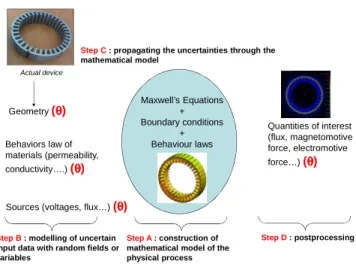
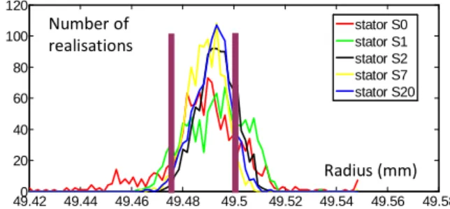
Uncertainty Quantification in Computational Electromagnetics: The stochastic approach

The experimental identification of a non-Gaussian positive matrix-valued random field in high stochastic dimension, using partial and limited ex- perimental data for a model

This doctoral thesis deals with the problem defined in the previous sec- tion and presents as main contributions: (i) the development of a mechanical- mathematical model to describe

The mean reduced nonlinear computational model, which results from the projection of all the linear, quadratic and cubic stiffness terms on this POD-basis is then explicitly

In the case for which uncertainties do only affect the linear stiffness terms, only the random elastic stiffness part is extracted from matrix [ K e ], using the nonlinear

Mais si les macrophages sont indispensables à la cicatrisation d’une plaie, c’est surtout car ils vont secréter une seconde vague de cytokines et de facteurs de croissance tel

Partially-intrusive Monte-Carlo methods to propagate uncertainty: ‣ By using sensitivity information and multi-level methods with polynomial chaos. expansion we demonstrate

Also, in the range of 2.75 F s (Safety Factor), the plots of probability density function for failure criterions intersect in each other according to the probability density

The purpose of this paper is to put forward an uncertain dimension reduction suitable for conducting a forward un- certainty propagation for the lift-off height of the H 2 Cabra