Contact process with random slowdowns: phase transition and hydrodynamic limits

(1)

HAL Id: tel-01100894

https://tel.archives-ouvertes.fr/tel-01100894

Submitted on 7 Jan 2015

HAL is a multi-disciplinary open access

archive for the deposit and dissemination of sci-entific research documents, whether they are pub-lished or not. The documents may come from teaching and research institutions in France or abroad, or from public or private research centers.

L’archive ouverte pluridisciplinaire HAL, est destinée au dépôt et à la diffusion de documents scientifiques de niveau recherche, publiés ou non, émanant des établissements d’enseignement et de recherche français ou étrangers, des laboratoires publics ou privés.

Distributed under a Creative Commons Attribution - NonCommercial - NoDerivatives| 4.0

transition and hydrodynamic limits

Kevin Kuoch

To cite this version:

Kevin Kuoch. Contact process with random slowdowns: phase transition and hydrodynamic limits. Probability [math.PR]. Université Paris Descartes, 2014. English. �tel-01100894�

(2)

école doctorale de sciences mathématiques de paris centre

THÈSE DE DOCTORAT

en vue de l’obtention du grade de

Docteur de l’Université Paris Descartes

Discipline : Mathématiques

présentée par

Kevin KUOCH

Processus de contact avec

ralentissements aléatoires

transition de phase et limites hydrodynamiques

Contact process with random slowdowns

phase transition and hydrodynamic limits

sous la direction d’Ellen SAADA

soutenue publiquement le 28 novembre 2014 devant le jury composé de

M. Thierry _Bodineau CNRS - École Polytechnique Rapporteur M. Thomas _Mountford École Polytechnique Fédérale de Lausanne Rapporteur

M. Mustapha _Mourragui Université de Rouen Examinateur

M. Frank Redig Technische Universiteit Delft Examinateur M. Rinaldo _Schinazi University of Colorado Colorado Springs Examinateur Mme Ellen _Saada CNRS - Université Paris Descartes Directrice

(3)

(4)

(5)

(6)

L’exercice des remerciements... loin d’être aussi facile que je ne l’imaginais, tant l’écosystème de la recherche est riche, tant les proches omniprésents sont nombreux. Il y a certainement des oublis et je prie les personnes concernées de m’en excuser.

Mes premiers mots vont naturellement à ma directrice de thèse, Ellen Saada, envers qui j’exprime ma plus profonde gratitude. Non seulement elle a été -incroyablement-patiente et humaine mais elle a su me mettre sur le chemin -malgré tous mes possibles déboires- avec les encouragements nécessaires. C’est une chance et un immense honneur d’avoir pu travailler avec elle, je ne serai que toujours friand de ses critiques et conseils tant ils sont chers et avisés.

À ceux qui me font l’honneur de composer le jury. Je remercie chaleureusement Ri-naldo Schinazi, pour avoir initié ce modèle mathématique et pour les discussions (malgré le décalage horaire) que nous avons pu partager. Il a su attiser ma curiosité et être une source d’inspiration considérable. Je tiens également à remercier Mustapha Mourragui, sa disponibilité, les innombrables aller-retours entre Paris et Rouen mais par dessus tout, sa convivialité et ses mots d’encouragement ont été d’un grand apport. Rapporter une thèse est loin d’être une part de gâteau. Je tiens à remercier Thierry Bodineau et Thomas Mountford d’avoir accepté de rapporter cette thèse, pour l’attention et les com-mentaires prodigués à ce manuscrit. J’aimerais aussi remercier Frank Redig de prendre part à ce jury et pour son chaleureux accueil aux Pays-Bas.

Ayant été le premier à avoir mis un article entre mes mains, j’aimerais remercier Amaury Lambert pour m’avoir initié à cette voie mais aussi pour s’être montré dispo-nible et m’avoir conforté dans des choix.

D’autre part, le long de mes études, j’ai eu la chance d’avoir pu suivre des personnes qui m’ont fait avancer jusque là aujourd’hui, en particulier, j’aimerais remercier Jean Bertoin, Marc Yor et Olivier Zindy, pour avoir été d’une notable attention et des sources d’inspiration.

Après ces années passées à Paris Descartes. Je remercie Annie Raoult, pour le soin qu’elle a porté au laboratoire. La terrasse étant sujette à beaucoup de pauses et de discussions : Merci à l’équipe de Probabilités, pour leur accueil et leurs conseils ; Merci à Joan Glaunès pour sa sympathie et les parties de tennis ; Merci également à Avner Bar-Hen, à Mikael Falconnet pour leur gentillesse.

Aux équipes administrative et informatique pour leurs aides diverses et variées : Merci à Marie-Hélène Gbaguidi toujours avec sourire et à l’écoute, Vincent Delos, Isa-belle Valéro, Christophe Castellani, Thierry Raedersdorff, Azedine Mani, Arnaud Meu-nier.

À l’équipe de biomathématiques qui m’a confié trois années d’enseignement. Je re-mercie profondément Simone Bénazeth pour son accueil et sa gentillesse. Merci éga-lement à Chantal Guihenneuc-Jouyaux, Ioannis Nicolis, Patrick Deschamps, Virginie Lasserre.

Merci aux doctorants et jeunes docteurs que j’ai pu voir ou qui me voient passer, ces ambiances de travail ou de non-travail, je vous les dois : Merci à Gaëlle C. (je t’en

(7)

Having recently landed in the Netherlands, I’d like to deeply thank Aernout van Enter and Daniel Valesin for their kindness and for taking care of my comfy arrival in Groningen.

Somehow I have had the chance to visit incredible places along past years and to take part in seminars, conferences and other events. I am very grateful to every person and institution that made it possible.

Trois années, c’est long. Certain(e)s ont dû entendre cette phrase à maintes reprises et je n’écrirais certainement pas ces mots si vous n’aviez pas été là. Il serait trop long d’exprimer à chacun(e) de vous mes sentiments et ma gratitude, vous les connaissez probablement déjà.

Mes plus doux remerciements à mes ami(e)s de très longue date (plus de la moitié de mes 25ans quand même !) : Mathieu J. et nos pinardises ; Guillaume de M. (vilain

merle) ; Timothée de G. (bulle) ; Jerôme T. et ses pin’s ; Marine L. ; Louis M. ; Hélène

de R. ; Guillaume L. (qui a osé suivre un de mes cours...) ; Mathieu B. ; Anne-Félice P. et ses bonjoirs ; Marine H. ; Nicolas I. ; Clémentine d’A. ; Hervé de S-P. ; Theodora B. ; Loup L. ; Bastien L. ; ce qui ne peut être évité, il faut parfois l’embrasser, à la mémoire d’Alexandre Z. pour ce qu’il a été et ce qu’il laisse derrière lui.

Je remercie chaleureusement Alex K. pour le plaisir de partager des discussions et moments aussi saugrenus qu’improbables avec lui.

Il est temps de retourner mes tendres remerciements à mon cher Daniel Kious (eh on y est arrivé finalement !), et à sa Famille pour leurs chaleureux accueils.

Merci à Samuel R. pour toutes nos inlassables conversations (et dégustations de whisky), j’espère qu’il nous en reste encore plein devant nous - j’attends avec impatience mon t-shirt Cyclop. Merci à Mario M. qui, sans conteste, fait le meilleur tiramisu que je connaisse. Merci à Raphaël L-R. pour entre autres ses conseils et son humour.

Merci à Pierre-Alban D. pour son soutien et être un si bon accolyte de fortune ; Merci à David B. non seulement pour avoir révolutionné le port du cardigan ; Merci à Diane T. et ses prestations de danse contemporaine ; Merci à Julie L. pour prendre soin de mes dents (j’attends toujours mon prochain rdv).

Merci aussi à Alicia H. et son rire détonant ; à Justyna S. pour sa gentillesse et son attention.

Enfin, et de tout mon cœur, je remercie mes parents et ma grande sœur, pour l’exemple qu’ils sont, pour toute la joie qu’ils me procurent, pour tout leur amour dont je suis -ô combien- insatiable.

(8)

“Then it doesn’t matter which way you go,” said the Cat. “—so long as I get somewhere,” Alice added as an explanation.

“Oh, you’re sure to do that," said the Cat, “if you only walk long enough.”

(9)

(10)

Dans cette thèse, on étudie un système de particules en interaction qui généralise un processus de contact, évoluant en environnement aléatoire. Le processus de contact peut être interprété comme un modèle de propagation d’une population ou d’une infection. La motivation de ce modèle provient de la biologie évolutive et de l’écologie comporte-mentale via la technique du mâle stérile, il s’agit de contrôler une population d’insectes en y introduisant des individus stérilisés de la même espèce : la progéniture d’une fe-melle et d’un individu stérile n’atteignant pas de maturité sexuelle, la population se voit réduite jusqu’à potentiellement s’éteindre.

Pour comprendre ce phénomène, on construit un modèle stochastique spatial sur un réseau dans lequel la population suit un processus de contact dont le taux de crois-sance est ralenti en présence d’individus stériles, qui forment un environnement aléatoire dynamique.

Une première partie de ce document explore la construction et les propriétés du processus sur le réseau Zd_{. On obtient des conditions de monotonie afin d’étudier la}

survie ou la mort du processus. On exhibe l’existence et l’unicité d’une transition de phase en fonction du taux d’introduction des individus stériles. D’autre part, lorsque

d “ 1 et cette fois en fixant l’environnement aléatoire initialement, on exhibe de nouvelles

conditions de survie et de mort du processus qui permettent d’expliciter des bornes numériques pour la transition de phase.

Une seconde partie concerne le comportement macroscopique du processus en étu-diant sa limite hydrodynamique lorsque l’évolution microscopique est plus complexe. On ajoute aux naissances et aux morts des déplacements de particules. Dans un pre-mier temps sur le tore de dimension d, on obtient à la limite un système d’équations de réaction-diffusion. Dans un second temps, on étudie le système en volume infini sur Zd, et en volume fini, dans un cylindre dont le bord est en contact avec des réservoirs stochastiques de densités différentes. Ceci modélise des phénomènes migratoires avec l’extérieur du domaine que l’on superpose à l’évolution. À la limite on obtient un sys-tème d’équations de réaction-diffusion, auquel s’ajoutent des conditions de Dirichlet aux bords en présence de réservoirs.

Mots-clefs. système de particules en interaction, modèle stochastique spatial, pro-cessus de contact, milieu aléatoire, attractivité, percolation, transition de phase, limite hydrodynamique, réservoirs.

(11)

(12)

In this thesis, we study an interacting particle system that generalizes a contact process, evolving in a random environment. The contact process can be interpreted as a spread of a population or an infection. The motivation of this model arises from behavioural ecology and evolutionary biology via the sterile insect technique ; its aim is to control a population by releasing sterile individuals of the same species : the progeny of a female and a sterile male does not reach sexual maturity, so that the population is reduced or potentially dies out.

To understand this phenomenon, we construct a stochastic spatial model on a lat-tice in which the evolution of the population is governed by a contact process whose growth rate is slowed down in presence of sterile individuals, shaping a dynamic random environment.

A first part of this document investigates the construction and the properties of the process on the lattice Zd. One obtains monotonicity conditions in order to study the survival or the extinction of the process. We exhibit the existence and uniqueness of a phase transition with respect to the release rate. On the other hand, when d “ 1 and now fixing initially the random environment, we get further survival and extinction conditions which yield explicit numerical bounds on the phase transition.

A second part concerns the macroscopic behaviour of the process by studying its hy-drodynamic limit when the microscopic evolution is more intricate. We add movements of particles to births and deaths. First on the d-dimensional torus, we derive a system of reaction-diffusion equations as a limit. Then, we study the system in infinite volume in Zd, and in a bounded cylinder whose boundaries are in contact with stochastic reser-voirs at different densities. As a limit, we obtain a non-linear system, with additionally Dirichlet boundary conditions in bounded domain.

Keywords. interacting particle system, spatial stochastic model, contact process, ran-dom environment, attractiveness, percolation, phase transition, hydrodynamic limit, re-servoirs.

(13)

(14)

1 Introduction 1

1.1 Interacting Particle Systems . . . 2

1.2 A short story of the contact process . . . 6

1.3 Hydrodynamic limits . . . 10

1.4 From life and nature . . . 12

1.5 The generalized contact process . . . 15

2 _{Phase transition on Z}d ₂₁ 2.1 Introduction . . . 21

2.2 Settings and results . . . 22

2.3 Graphical construction . . . 28

2.4 Attractiveness and stochastic order . . . 31

2.5 Phase transition . . . 47

2.6 The critical process dies out . . . 54

2.7 The mean-field model . . . 65

3 Survival and extinction conditions in quenched environment 69 3.1 Introduction . . . 69

3.2 Settings and results . . . 70

3.3 Random growth on vertices . . . 72

3.4 Random growth on oriented edges . . . 76

3.5 Numerical bounds on the transitional phase . . . 79

4 Hydrodynamic limit on the torus 81 4.1 Introduction . . . 81

4.2 Notations and Results . . . 82

4.3 The hydrodynamic limit . . . 86

4.4 Proof of the replacement lemma . . . 96

4.A Construction of an auxiliary process . . . 102

4.B Properties of measures . . . 107

4.C Quadratic variations computations . . . 110

4.D Topology of the Skorohod space . . . 113

5 Hydrodynamic limits of a generalized contact process with stochastic reservoirs or in infinite volume 115 5.1 Introduction . . . 116

5.2 Notation and Results . . . 118

5.3 Proof of the specific entropy (Theorem 5.2.1) . . . 130

5.4 Hydrodynamics in a bounded domain . . . 137

5.5 Empirical currents . . . 146

5.6 Hydrodynamics in infinite volume . . . 148

5.7 Uniqueness of weak solutions . . . 149

(15)

5.B Quadratic variations computations . . . 157 5.C Estimates in bounded domain . . . 160

Perspectives 163

(16)

1

Introduction

This thesis examines two different aspects of a generalized contact process. In a microscopic scale, we study survival or extinction of the process with respect to varying parameters. Then, we go to a macroscopic scale and establish hydrodynamic limits, where in the dynamics of the underlying process we add displacements of particles and further on migratory phenomena.

In this chapter, we introduce some general settings we shall make use of, first on interacting particle systems in Section 1.1 and then on the contact process in Section 1.2. After what, in Section 1.4, we develop shortly the big picture of the sterile insect technique. In Section 1.5, we describe a generalized contact process and our results that lead to an understanding of this competition model.

(17)

1.1 Interacting Particle Systems

Interacting particle systems are a class of Markov processes that arose in the early seventies due to pioneering works by F. Spitzer [70, 71] and R.L. Dobrushin [16]. They have provided a framework that describes the space-time evolution of an infinity of indistinguishable particles governed by a strong random and local interaction.

This particular class of stochastic processes comes up in various areas of applications : physics, biology, computer science, economics and sociology,... that dictate the nature of the randomness of the processes.

1.1.1 The setup

As a preparation, one first reviews some necessary background theory about inter-acting particle systems. For further contents on the topic, one refers the reader to T.M. Liggett’s books [58, 57].

State spaces are of the form Ω “ FS_{, where F is discrete and finite, S is a countable}

set of sites. Note that Ω is compact in the product topology. A configuration ζ P Ω is described by the state of each site x of the graph S, given at time t by ζtpxq P F . For

each ζ P Ω and T Ă S, the local dynamics of the system is depicted by a collection of transition measures cTpζ, dαq, assumed to be finite and positive on FT. Assume

further that the mapping ζ ÞÑ cTpζ, dαq is continuous from Ω to the space of finite

measures on FT _{with the topology of weak convergence. If ζ is the current configuration,}

a transition of state or flip involving the coordinates in T occurs at rate cTpζ, FTq and

cTpζ, dαq{cTpζ, FTq is the distribution of the resulted configuration restricted to T .

We will use the notation Pζ for the distribution of the process pζtqtě0 starting from

the initial configuration ζ, and Eζ _{will denote the corresponding expectation. The}

infi-nitesimal description of a process ζ P Ω is given by its generator L, a linear unboun-ded operator defined on an appropriate dense domain DpΩq of the space of functions

f : Ω Ñ R. For any cylinder function f , i.e. that depends only on finitely many

coordi-nates, L is defined by Lf pζq “ÿ T ż Ω cTpζ, dαq`fpζαq ´ f pζq˘, (1.1.1)

where ζα _{is obtained from ζ only by flipping the coordinates in T , that is, for α P F}T_,

ζα “" ζpxq if x R T,

αpxq if x P T.

The series converges provided that cTp., .q satisfies natural summability conditions.

Let CpΩq be the space of continuous real-valued functions on Ω equipped with the uniform norm. All the processes we consider here have the Feller property (i.e. strong Markov processes whose transition measures are weakly continuous in the initial state) so that the semigroup St of the process on CpΩq is well defined :

(18)

Theorem 1.1.1. Suppose tSt, t ą 0u is a Markov semigroup on CpΩq. Then there exists

a unique Markov process tPζ_{, ζ P Ωu such that}

Stf pζq “ Eζf pζtq

for all f P CpΩq, ζ P Ω and t ě 0.

The link binding the infinitesimal description of the process (generator) to the time-evolution of the process (semigroup) is given by the Hille-Yosida theory set in the Banach space CpΩq.

Theorem 1.1.2 (Hille-Yosida). There is a one-to-one correspondence between Markov generators on CpΩq and Markov semigroups on CpΩq. This correspondence is given by

1. DpΩq “ " f P CpΩq : lim tÓ0 Stf ´ f t exists * , and Lf “ lim tÓ0 Stf ´ f t , f PDpΩq. 2. for t ě 0, Stf “ lim nÑ8pf ´ t nLf q ´n , f P CpΩq.

Relying on the Hille-Yosida theory, the following result states sufficient conditions for the existence of an infinite particle system.

Theorem 1.1.3 (T.M. Liggett (1972)). Assume that

sup xPS ÿ T Qx sup ´ cTpζ, FTq : ζ P Ω ¯ ă 8 and sup xPS ÿ T Qx ÿ u‰x sup ´

}cTpζ1, dαq ´ cTpζ2, dαq}T : ζ1pyq “ ζ2pyq for all y ‰ u

¯ ă 8

where } ¨ }T stands for the total variation norm of a measure on FT. Then the closure

L of L defined in (1.1.1) is the generator of a Feller Markov process pζtqtě0 on Ω. In

particular, if f is a cylinder function then,

Lf “ lim

tÑ0

Stf ´ f

t ,

LStf “ StLf

and uptq “ Stf is the unique solution to the evolution equation

Btuptq “ Luptq, up0q “ f. (1.1.2)

Let P be the set of probability measures on Ω equipped with the topology of weak convergence, i.e. µnÑ µ in P if and only if ż Ω f dµn Ñ ż Ω f dµ

for all f P CpΩq. Note that the compactness of Ω implies the compactness of P in this induced topology.

(19)

1.1.2 Invariant measures

Study of interacting particle systems involves use of their invariant measures and ideally, convergence to them. If µ is a probability measure on Ω, the distribution of ζt

with initial distribution µ is denoted by µSt and is defined by

ż Ω f dpµStq “ ż Ω Stf dµ, f P CpΩq.

By the Riesz Representation theorem, this relation defines uniquely µSt. The measure

µ is invariant with respect to the process if µSt “ µ for all t ą 0. Denote by I the set

of all invariant measures. Furthermore,

Theorem 1.1.4 (Proposition 1.8 [58]). i. µ P I if and only if

ż

Ω

Lf dµ “ 0, for all cylinder functions f.

ii. I is compact, convex and non-empty.

iii. I is the closed convex hull of its extreme points. iv. Let µ P P. If µ :“ lim

tÑ8µSt exists, then µ P I.

Remark that a process always has at least one invariant measure. This measure might satisfy a symmetry property called reversibility that allows simpler computations or even, further results. A probability measure µ on Ω is reversible for the process if

ż Ω f Stgdµ “ ż Ω gStf dµ, for all f, g P CpΩq or equivalently, ż Ω f Lgdµ “ ż Ω

gLf dµ, for all cylinder functions f, g.

1.1.3 Coupling and stochastic order

A coupling is a construction of two (or even more) stochastic processes on a common probability space. To make use of this powerful tool, we will deal with several topics that are closely connected with coupling such as stochastic order relations between proba-bility measures, monotone processes and correlation inequalities. These useful relations allow us to compare processes, so that one can deduce properties from one to another by domino effect.

Assuming that F is totally ordered, the state space Ω is a partially ordered set, with partial order given by

ζ ď ζ1 _{if for all x P S, ζpxq ď ζ}1

(20)

where this last inequality refers to the order on F . A function f P CpΩq is increasing if

ζ ď ζ1

ñ f pζq ď f pζ1q.

This leads naturally to define the stochastic order between two probability measures µ1

and µ2 on Ω, that is, µ2 is stochastically larger than µ1, written µ1 ď µ2 if :

ż

Ω

f dµ1 ď

ż

Ω

f dµ2 for any increasing function f on Ω.

A necessary and sufficient condition for a semigroup, acting on measures, to preserve the ordering on Ω is given by

Theorem 1.1.5 (Theorem 2.2 [57]). For a Feller process on Ω with semigroup St, the

following two statements are equivalent :

a. If f is an increasing function on Ω then Stf is an increasing function of Ω for all

t ě 0.

b. If µ1 ď µ2 then µ1Stď µ2St for all t ě 0.

Stochastic order between two particle systems pζtqtě0 and pζt1qtě0 is given by the

existence of a coupled process pζt, ζt1qtě0 on the probability space Ω ˆ Ω that preserves

the order between their initial configurations, that is, if ζ0 ď ζ01 then ζtď ζt1 a.s. for all

t ą 0. Such a coupling is said to be increasing and ζ1

t is said to be stochastically larger

than ζt. When pζtqtě0 and pζt1qtě0 are two copies of the same process, we say the process

is attractive.

The following result gives the connection between coupling and stochastic order.

Theorem 1.1.6 (Theorem 2.4 [58]). Let µ1 and µ2 be probability measures on Ω. Then

µ2 is stochastically larger than µ1 if and only if there exists a coupling pζ, ζ1q such that ζ

has distribution µ1, ζ1 has distribution µ2 and ζ ď ζ1 almost surely, that is, there exists

a measure ν on Ω such that

νtpζ, ζ1 q : ζ P Au “ µ1pAq νtpζ, ζ1 q : ζ1 P Au “ µ2pAq νtpζ, ζ1 q : ζ ď ζ1u “ 1

Furthermore, we will consider different types of stochastic processes : pξtqtě0 (basic) contact process

pξt, ωtqtě0 contact process in dynamic random environment

(21)

1.2 A short story of the contact process

Introduced by T.E. Harris in 1974 [39], the contact process on the graph S with growth rate λ1 is an interacting particle system pξtqtě0 on t0, 1uS, whose dynamics is

given by the following transition measure : the involved sets T are singletons T “ txu and, cTpξ, dαq “ " λ1n1px, ξqδt1u if ξpxq “ 0, δt0u if ξpxq “ 1, (1.2.1) where nipx, ξq “ ř yPS:|y´x|“1

1tξpyq “ 1u stands for the number of neighbours of site x

that are in state i. Here | ¨ | refers to the maximum norm : |x| “ max

1ďjďd|xj|, for x P R d_.

Denote by Pλ1 the law of the contact process with growth rate λ1.

It is usually interpreted as the spread of a population, an infection or a rumour. Regarded as an infection, infected sites (in state 1) become healthy spontaneously after a unit exponential time while healthy sites (state 0) become infected at some rate, pro-portional to the number of their infected neighbours.

General theory about the contact process is finely exposed by T.M Liggett [58] for results from 1974 to 1985, [57] for results after 1985 and by R. Durrett [18] as well.

1.2.1 Construction of the process

Let A be a subset of S. Define ξA

t as the process starting from the initial configuration

ξ0 “ 1A. Configurations ξ P t0, 1uS are commonly identified with subsets of S via

ΞA_t “ tx P S : ξtApxq “ 1u,

regarded as the set of occupied sites at time t. When A “ t0u, we will omit the exponent. As a consequence of Theorem 1.1.3, the transition measure cTpξ, dαq uniquely defines a

Markov process, so that the infinitesimal generator of the contact process is defined for any cylinder function f on t0, 1uS _by

L1f pξq “ ÿ xPS ż Ω cTpξ, dαqrf pξαq ´ f pξqs (1.2.2)

Graphical representation The graphical construction of the contact process is due to T.E. Harris [40]. The idea is to construct a percolation structure on which to define the process, lending itself to the use of the theory of percolation (see G. Grimmett [33]). To carry out this representation, for each pair px, yq P S2 _{that are joined by an edge in}

S, let tTnx,y, n ě 1u be the arrival times of independent rate λ1 Poisson processes and for

each x P S, let tDx

(22)

Both families of Poisson processes are mutually independent. Now, think of the space-time diagram S ˆ r0, 8q. At space-time t “ Dx

n, put a death symbol “x” at px, tq P S ˆ r0, 8q.

At time t “ Tx,y

n , draw an arrow from px, tq to py, tq.

By way of illustration, see Figure 1.1.

-2 -1 0 1 2

time

0

t

Figure 1.1: The graphical representation for the contact process on Z1ˆ R`

For s ď t, there exists an active path in the space-time picture S ˆ r0, 8q from px, sq to py, tq, written px, sq Ñ py, tq, if there exists a sequence of times s “ s0 ă s1 ă ... ă

sn´1ă sn “ t and spatial locations x “ x0, x1, ..., xn “ y such that

i. for i “ 1, ..., n, there is an arrow from xi´1 to xi at time si.

ii. for i “ 0, ..., n ´ 1, the vertical segments txiu ˆ psi, si`1q contain no death symbol.

In words, an active path is a connected oriented path that moves forward in time wi-thout crossing a death symbol and along the directions of the arrows. For instance, in Figure 1.1, there is an active path from p0, 0q to p1, tq. The contact process with initial configuration A Ă S is obtained by setting

AA_t :“ ty P S : Dx P A such that px, 0q Ñ py, tqu Therefore, in our previous example, At0ut “ t1u.

The graphical construction provides a joint coupling of contact models with different transition rates : let λp1q₁ ď λp2q1 , if we constructed the process with rate λ

p2q

1 and we keep

each arrow with probability λp1q₁ {λp2q1 , by the thinning property of the Poisson processes,

(23)

Thus, one has a non-decreasing growth with respect to λ1. On the other hand, it also

provides a monotone coupling :

A Ă B ñ AA_t Ă ABt ,

Therefore, the contact process is attractive and it also follows from the graphical construc-tion that the contact process is additive (see D. Griffeath [32]) :

AAYB_t “ AA_t Y AB_t .

1.2.2 Upper invariant measure and duality

Since the partial order on Ω defined in (1.1.3) induces one on the set of probability measures on Ω, there will be a lowest and largest element on I with respect to this partial order.

If 0 denotes the configuration identically equal to 0, since 0 is an absorbing state then δ0 is called the lower invariant measure for the contact process. The upper invariant

measure can be constructed using attractiveness : choose the initial configuration as the biggest possible one, i.e. starting from Ξ0 “ S, and let µt be the distribution of ξt, so

that µ0 “ δ1. Then µt ď µ0. By attractiveness and applying the Markov property, we

have µt`s ď µt for all s ą 0. Therefore, t ÞÑ µt is decreasing and in particular, for every

increasing function f on Ω, the map t ÞÑ ş_Ωf dµt is decreasing as well. Since PpΩq is

compact for the weak topology, the limiting distribution

µ :“ lim

tÑ8µt

exists and is the upper invariant measure of the process. It is invariant as a limiting measure for the Markov process by Theorem 1.1.4. In particular, the measure µ has positive correlations.

Correlation inequalities will be crucial property in Section 2.6 where we will work in arbitrary large but finite spaces. A probability measure µ on Ω has positive correlations if ż Ω f gdµ ě ż Ω f dµ ż Ω gdµ,

for all increasing functions f, g on Ω. A sufficient condition for a measure to have positive correlations is given by the following result.

Theorem 1.2.1 (C. Fortuin, P. Kasteleyn and J. Ginibre [29]). Suppose S is finite. Let µ be a probability measure on Ω such that for all ζ, ζ1

P X

µ1pmaxpζ, ζ1qqµ2pminpζ, ζ1qq ě µ1pζqµ2pζ1q

(24)

One essential property satisfied by the contact process is that it is self-dual [34, Proposition 6.5], that is, the dual process is again a contact process. For A, B Ă S,

Pλ1pΞ

A

t X B ‰ Hq “ Pλ1pΞ

B

t X A ‰ Hq (1.2.3)

This property allows us to link an equality relation between survival probability and density of 1’s under the upper invariant measure. Indeed, since tΞt0ut`1 X S ‰ Hu Ă

tΞt0ut X S ‰ Hu for all t ě 0, t ÞÑ tΞ t0u t X S ‰ Hu is non-increasing, lim tÑ8Pλ1pΞ t0u t X S ‰ Hq “ Pλ1p@t ě 0, Ξ t0u t ‰ Hq

By self-duality, applying (1.2.3) with A “ t0u and B “ S, one obtains Pλ1pΞ

t0u

t X S ‰ Hq “ Pλ1pΞ

S

t X t0u ‰ Hq.

The right-hand side is Pλ1pΞ

S

tp0q “ 1q, and by weak convergence of µ0 to µ, one has

lim

tÑ8Pλ1pΞ S

tp0q “ 1q “ ¯µtξ : ξp0q “ 1u

where µ stands for the upper invariant measure of pξtqtě0. By translation invariance of

µ, lim tÑ8Pλ1pΞ t0u t X S ‰ Hq “ lim_tÑ8Pλ1pξ S tp0q “ 1q “ ¯µtξ : ξpxq “ 1u (1.2.4)

1.2.3 Survival and extinction

A key feature of the contact process lies in the fact its growth does not evolve spon-taneously but depends on some neighbourhood. In words, the configuration 0 is a trap and a natural question is whether the individuals survive, that is, if there is infinitely often a site in state 1. The main feature of the contact process is that it exhibits a phase transition in the following way.

Define the survival event of the process by t@t ě 0, Ξt ‰ Hu with the initial

configuration ξ0 “ 1t0u. The contact process is said to die out if

Pλ1p@t ě 0, Ξt‰ Hq “ 0

and to survive strongly if

Pλ1p lim_tÑ8ξtp0q “ 1q ą 0.

The process is said to survive weakly if it survives but not strongly, that is, Pλ1p@t ě 0, Ξt ‰ Hq ą 0.

Using these definitions and monotonicity, we are now ready to define the two following critical values :

(25)

and

λs“ inftλ1 : Pλ1p lim_tÑ8ξtp0q “ 1q ą 0u. (1.2.6)

for which, the process

dies out if λ1 ă λc survives weakly if λc ă λ1 ă λs survives strongly if λ1 ą λs Since t lim tÑ8ξtp0q “ 1u Ă t@t ě 0 Ξt‰ Hu,

if the process survives weakly then it survives strongly thus λc ď λs.

On the d´dimensional integer lattice Zd, one of the most important results about the contact process is the existence and uniqueness of a critical value λc“ λs.

Theorem 1.2.2 (T.E. Harris [39]). There exists a critical value λc P p0, 8q such that

the contact process survives if λ1 ą λc and dies out if λ1 ă λc, i.e.

Pλ1p@t ě 0, Ξt‰ Hq “ 0 if λ1 ă λc,

Pλ1p@t ě 0, Ξt‰ Hq ą 0 if λ1 ą λc.

After having been an open question during about fifteen years, the critical behaviour has been given by

Theorem 1.2.3 (C. Bezuidenhout and G.R. Grimmett [5]). The critical contact process dies out, that is,

Pλcp@t ě 0, Ξt ‰ Hq “ 0.

R. Holley and T.M. Liggett [41] proved λc ď 2 in the one-dimensional case. An

improved upper bound 1.942 was given by T.M. Liggett [54]. More generally, one has for the general case d ě 1,

p2d ´ 1q´1 ď λcď 2d´1,

see N. Konno [47] for further information on bounds of the contact process.

1.3 Hydrodynamic limits

Hydrodynamic limits are a device that arose in statistical physics to derive deter-ministic macroscopic evolution laws assuming the underlying microscopic dynamics are stochastic.

By way of illustration, consider the evolution of a system constituted of a large number of components (such as a fluid), one can examine and characterize the equi-librium states of the system through macroscopic quantities (such as temperature or pressure). Now, investigating the fluid in a volume which is small macroscopically but

(26)

large microscopically, the system is close to an equilibrium state and characterized by some spatial parameter. As the local equilibrium picture should evolve in a smooth way, at some time t the system is close to a new equilibrium state now characterized by a parameter depending on space and time. This space-time parameter evolves smoothly in time according to a partial differential equation, the hydrodynamic equation.

To take the limit from the microscopic to the macroscopic system, we need to in-troduce a suitable space-time scaling. Consider a microscopic space SN embedded in

a corresponding macroscopic space S (e.g. SN “ pZ{N Zqd and S “ pR{Zqd) so each

microscopic vertex x P SN is associated to a macroscopic vertex x{N P S. Therefore,

distance between particles converges to zero. Besides, we renormalize the time by linking a microscopic time t to a macroscopic time tθpN q (e.g. θpN q “ N2), since more time is needed in the macroscopic scale to observe movements of particles.

To investigate the hydrodynamic behaviour of interacting particle systems we shall prove that starting from a sequence of measures associated to some initial density profile

ρ0, in the following sense

lim N Ñ8µN ˜ ˇ ˇ ˇ 1 Nd ÿ xPSN Gpx{N qηpxq ´ ż S Gpuqρ0puqdu ˇ ˇ ˇ ą δ ¸ “ 0 (1.3.1)

for any δ ą 0 and continuous function G : S Ñ R, then at some renormalized time

tθpN q, we obtain a state StθpN qµN associated to a new density profile ρtp¨q that is a

weak solution of a partial differential equation. That is, lim N Ñ8µN ˜ ˇ ˇ ˇ 1 Nd ÿ xPSN Gpx{N qηtθpN qpxq ´ ż S Gpuqρtpuqdu ˇ ˇ ˇ ą δ ¸ “ 0. (1.3.2) In other words, the sequence of measures µN integrates the density ρtat the macroscopic

point u P S in the same way than an equilibrium measure of density γpuq does.

Since we shall work in a fixed space as N increases, we will examine the time-evolution of the empirical measures associated to the interacting particle system : for a configuration η P Ω, define the empirical measure πNpηq on S associated to η by

πNpηq “ N´d ÿ

xPSN

ηpxqδx{N, (1.3.3)

where δx represents the Dirac measure concentrated on x. This way, we can express

(1.3.2) in terms of the empirical density, by integrating G with respect to πN_{. Since}

there is a one-to-one correspondence between a configuration η and empirical measure

πNpηq, the measure πNt inherits the Markov property.

The goal to derive the hydrodynamic limits is to prove the empirical measure πN t

converges in probability to an absolutely continuous measure ρpt, uqdu where ρtpuq is

the solution of a partial differential equation with initial condition ρ0.

Monographs dealing with hydrodynamic limits include A. De Masi and E. Presutti [15], H. Spohn [72] C. Kipnis and C. Landim [42].

(27)

1.4 From life and nature

During the last decades, a better understanding of biological phenomena has arisen the need to study stochastic spatial processes. Authors such as R. Durrett, R. Schinazi, or J. Schweinsberg have deemed the relation of interacting particle systems to biological, ecological and medical frameworks. A quick interesting overview may be found in joint papers of R. Durrett with the biologist S. Levin [21, 22], and [20].

In this document, the biological phenomenon we are concerned is the so-called Sterile insect technique (SIT). Due to entomologists R.C. Bushland and E.F. Knipling’s works [46] in the fifties, it is a pest control method whereby sterile individuals of the popula-tion to either regulate or eradicate are released. While sterile males compete with wild males, they eventually mate with (wild) females preventing the apparition of progenies. By repeated releases, we should be able to cause a variety of outcomes ranging from reduction to extinction.

1.4.1 The sterile insect technique

In the thirties and forties, the idea of designing a gene that actively spreads through a pest population without conveying some fitness advantage had arisen independently by A. S. Serebrovskii (Moscow State University), F. L. Vanderplank (Bristol Zoo and Tanzania Research Department) and E. F. Knipling (United States Department of Agri-culture). Serebrovskii and Vanderplank both sought to achieve pest control through par-tial sterility that occurs when different species or genetic strains were hybridized (using chromosomal translocations or crossing) : competition between two interbreeding strains doesn’t favour the fitter group, involving the genetic property called under-dominance which can actually cause the strain with greater fitness to die out.

Discovery and first success story. Discovery of induced mutagenesis by 1946 No-bel Prize H.J. Muller conducted Bushland and Knipling to use ionizing radiation in the sterilization process to get rid of the new world screw-worm fly (Cochliomyia hominivo-rax).

After successful eradication programs carried out in Curaçao and Florida in the late fifties, the technique was applied during the next decades to eradicate the screw-worm from the USA, Mexico, and Central America to Panama, until it has been declared a fly-free area.

The big picture. Food safety, quality and biodiversity have required demands at national and international levels for the development and introduction of area-wide (and biological approaches) for integrated management of pest control.

Fruit flies are a major interference in the marketing of fruit and vegetable commo-dities, preventing therefore important economic developments. The Mediterranean fruit

(28)

fly (medfly) is a notorious insect pest threatening multi-million commodities export trade throughout the world.

In the seventies, a first large-scale program stopped the invasion of the medfly from Central America. Eradication from Mexico and maintaining the country free of this pest at an annual cost of US$ 8 million, has protected fruit and vegetable export markets of close to US$ 1 billion a year.

In Japan, the SIT was employed in the eighties and nineties to eradicate the melon fly in Okinawa and south-western islands, permitting access for fruits and vegetables produced in these islands to the main markets in the mainland. A program with Peru operates in Argentina, northern Chile and southern Peru. Chilean fruits have entered the US market for exports estimated to up to US$ 500 million per year.

More recently, the SIT is increasingly applied with eradication programs of fruit flies ongoing in Middle-East (Israel, Jordan, Palestine), South Africa, and Thailand ; in preparation in Brazil, Portugal, Spain, and Tunisia.

Economic benefits have been confirmed so that for medflies and other fruit flies, the current worldwide production capacity of sterile individuals has reached several billion a week.

Future trends. Lauded for its attributes in terms of economics, environment and safety, the technique has successfully been able to get rid of populations threatening livestocks, fruits, vegetables, and crops. But besides economic reasons to involve SIT, public health issues have induced governments to request supports from International Atomic Energy Agency (IAEA) and Food and Agriculture Organization of the United Nations (FAO) for SIT initiatives to stem vector-borne diseases.

1.4.2 Time to unleash the mozzies ?

Thinking about the deadliest animal in the world, mosquitoes would not hit our minds. But one estimates about 1 million people per year die from mosquito-borne diseases, such as malaria, dengue fever, etc ... [Source : World health organization].

Urbanisation, globalisation and climate change have accelerated the spread and in-creased the number of outbreaks of new mosquito-borne diseases, such as the dengue.

Considered as the fastest growing disease, dengue fever is currently not cured by any vaccine or effective antiviral drug, meaning that mosquito control is the only viable option to control the disease at short notice. The SIT has the potential to reduce the targeted mosquitoes population to a level below which the disease is not transmitted. A first trial using sterile mosquitoes was conducted in El Salvador in the seventies, where 4.4 million sterile individuals were released in a 15 square km area over 22 weeks, eradicating successfully the targeted population. Going on a much larger area, total suppress of the population failed due to an immigration of local mosquitoes into the trial area.

(29)

Figure 1.2: Average number of dengue cases in most highly endemic countries as re-ported to WHO 2004-2010.

Being the highest endemic country of dengue, the brazilian government is highly concerned by the expansion of the dengue fever. According to pilot-scale releases in the state of Bahia started in june 2013, releases of genetically modified mosquitoes resulted in a 96% reduction of the wild population in the target area after 6 months- level maintained for a further 7 months using continued releases, at reduced rates, to avoid re-infestation.

The National Technical Commission for Biosecurity (CTNBio) in Brazil recently approved (april 2014) the commercial release of genetically modified mosquitoes in a bid to curb outbreaks of dengue fever. As of july 2014, the research program in the state of Bahia is waiting for an approval granted by the Brazilian Health Surveillance Agency (ANVISA) to ensue a scaling-up of the program. [Source : Comissão Técnica Nacional de Biossegurança (CTNBio), Agência Nacional de Vigilância Sanitária (ANVISA).]

1.4.3 Past mathematical models

Even if models of population dynamics are typically posed as difference or differential equations, such as predator-prey systems (whose Nicholson-Bailey and Lotka-Volterra models are the work horses), stochastic models give additional information on the expec-ted variability of the resulting control. Some of them were developed by Kojima (1971), Bogyo (1975), Costello and Taylor (1975), Taylor (1976) and Kimanani and Odhiambo (1993), and they confirmed the former results of Knipling (1955) [46] and others that used deterministic models.

(30)

foresha-dowing most future modelling developments. The key feature of Knipling’s models, and found in most of all subsequent models, is the ratio of fertile males to all males in the population. Simply modifying a geometric growth model,

Ft`1“ λpWt{pS ` WtqqFt

where Ft and Wt is the population size of females and wild males at time t, λ is the

growth rate per generation, R is the release rate of sterile individuals each generation. This yields an unstable positive equilibrium for F when R “ R˚, where R˚ “ F pλ ´ 1q denotes the critical release rate, so that if R ą R˚ then the population collapses while if R ă R˚ then the population will increase indefinitely.

The question of the competitive ability of males was modelled amongst others by Berryman (1967), Bogyo et al. (1971), Berryman et al. (1973), Ito (1977), and Barclay (1982) all showing that the critical release rate increases as the competitive ability of sterilized individuals decreases.

For a general overview of the technique, we refer the reader to [27].

1.5 The generalized contact process

In the further chapters, one constructs a contact process in random environment to lead a better understanding of this ecological phenomenon. Fix growth parameters λ1,

λ2 and release rate r.

One introduces the contact process in dynamic random environment (CP-DRE) on the graph S with parameters set pλ1, λ2, rq as an interacting particle system pξt, ωtqtě0P

pt0, 1u ˆ t0, 1uqS that evolves through the following dynamics. The environment part pωtqtě0 evolves independently according to

0 Ñ 1 at rate r, 1 Ñ 0 at rate 1, (1.5.1) while the contact process part evolves at x P S according to

0 Ñ 1 at rate ř

y:}y´x}“1

´

λ1ξpyqp1 ´ ωpyqq ` λ2ξpyqωpyq

¯

,

1 Ñ 0 at rate 1.

(1.5.2)

As we shall see, the most interesting case corresponds to λ2 ď λcă λ1, where λcdenotes

the critical value of the (basic) contact process. In words, the CP-DRE depicts a basic contact process whose growth rate is either subcritical or supercritical according to a time-evolving random environment which is parametrized by a rate r.

In our framework, one understands the environment as the space-time evolution of the sterile population released at rate r while the contact process stands for the wild population. When mixed up on a site, a competition between the two species occurs,

(31)

slowing down the growth of the wild individuals to a subcritical rate λ2, if not, the wild

individuals perform a supercritical contact process. Each individual dies spontaneously at rate 1.

In a traditional overview, the contact process part describes the spread of an infec-tion, so that the environment is thought of as being an immune response, attempting to slow down the expansion of the infection.

We also make use of a different but equivalent outlook of this process, that is, one constructs a (single) multitype contact process pηtqtě0on t0, 1, 2, 3uS, where each of these

values corresponds to a possible combination of values taken by the process pξt, ωtqtě0.

This way, a site x of S is empty if in state 0, occupied by type-1 individuals if in state 1, by type-2 individuals if in state 2 and occupied by both types simultaneously if in state 3.

It is important to underline that a site is occupied by a type of individuals and not as usual, by the number of individuals present standing on. We shall therefore rather think of a multicolour system.

Biologically speaking, one interprets the type-1 individuals as being the wild in-dividuals and the type-2 as being the sterile inin-dividuals. Sites in state 3 containing both types represent sites where competition occurs. We say that sites in state 1 or 3 constitute the wild population.

Furthermore, in the multitype outlook we consider two kinds of action for the type-2 individuals that are reducing the growth rate in sites in state 3. In a so-called asymmetric case, type-2 individuals prevent births from occurring in sites they are standing on. Call it symmetric otherwise. Common transition rates for both cases at site x are given by

0 Ñ 1 at rate λ1n1px, ηq ` λ2n3px, ηq 1 Ñ 0 at rate 1

0 Ñ 2 at rate r 2 Ñ 0 at rate 1

1 Ñ 3 at rate r 3 Ñ 1 at rate 1

3 Ñ 2 at rate 1

(1.5.3)

in which one adds the following transition in the symmetric case

2 Ñ 3 at rate λ1n1px, ηq ` λ2n3px, ηq. (1.5.4)

As competition occurs in sites in state 3, growth rate λ2has to be lower than growth rate

λ1 of sites in state 1 where only type-1 individuals live. One thus makes the hypothesis :

λ2 ă λ1. (1.5.5)

Here, since the presence of type-2 individuals dictate the growth rate of type-1 indi-viduals, to even inhibit births in the asymmetric case, the type-2 individuals shape a dynamic random environment for the type-1 individuals.

(32)

Both outlooks of the process are linked by the following relations :

ηpxq “ 0 Ø p1 ´ ξpxqqp1 ´ ωpxqq “ 1 ηpxq “ 1 Ø ξpxqp1 ´ ωpxqq “ 1 ηpxq “ 2 Ø p1 ´ ξpxqqωpxq “ 1 ηpxq “ 3 Ø ξpxqωpxq “ 1

In a microscopic scale, we examine survival and extinction conditions for the popula-tion, after what, taking the hydrodynamic limit, we study the behaviour of the densities of each type of population at a macroscopic scale.

1.5.1 Phase transition in dynamic random environment

Set S as the d-dimensional integer lattice Zd_{, d ě 1. In Chapter 2, one investigates}

how the release rate affects the behaviour of the process.

First, we point out general properties of the system, such as necessary and sufficient conditions for the process to be monotone, then, only sufficient conditions to be in line with the construction of the process. The tricky part to prove these conditions lies in the definition of an order on the state space t0, 1, 2, 3uZd_{, since a value on a given site}

does not correspond to the number of particles but a type. This is the interest of the next result.

Proposition. The symmetric multitype process is monotone, in the sense that, one can construct on a same probability space two symmetric multitype processes pηp1qt qtě0 and

pηtp2qqtě0 with respective parameters pλ p1q 1 , λ p1q 2 , rp1qq and pλ p2q 1 , λ p2q 2 , rp2qq, such that ηp1q₀ ď ηp2q0 ùñ η p1q t ď η p2q

t a.s. for all t ě 0 (1.5.6)

if and only if both parameters sets satisfy 1. λp1q₂ ď λp1q1 , 2. λp2q₂ ď λp2q1 , 3. λp1q₁ ď λp2q1 , 4. λp1q₂ ď λp2q2 , 5. rp1q _{ě r}p2q 6. λp1q₁ ď 1, 7. λp1q₂ ď 1, 8. rp1q _{ě 1.}

Essentials of SIT concern the control of the population by releasing sterile indivi-duals, the question we address now is for which values of r does the wild population survive or die out ? For this, we prove the existence and uniqueness of a phase transition with respect to the release rate r for fixed growth rates λ1 and λ2. The most interesting

cases are discussed in the following results :

Theorem. Suppose λ2 ď λc ă λ1 fixed. Consider the symmetric multitype process.

There exists a unique critical value rcP p0, 8q such that the wild population survives if

r ă rc and dies out if r ě rc.

Theorem. Suppose λc ă λ1 fixed. Consider the asymmetric multitype process. There

exists a unique critical value scP p0, 8q such that the wild population survives if r ă sc

(33)

This actually confirms the former conclusions done by Knipling (1955) in a determi-nistic model mentioned in Section 1.4.

Proofs strongly rely on the use of graphical representations and comparison with percolation processes that introduced M. Bramson and R. Durrett [11]. Using dynamic renormalization techniques from G. Grimmett et al. [2, 35], we are in particular able to describe the behaviour of the critical process. As a consequence, this allows us to discuss the competitive ability of the sterile individuals which was biologically exhibited (as mentioned in Section 1.4) : one shows the critical value increases as the competitiveness of the sterilized population decreases or as the fitness of the wild population increases. We end up this chapter by considering the associated mean-field equations. This shows us a dynamical system featuring the densities of each type of individuals. There, we can explicit equilibria and mainly explicit numerical bounds on the transitional phase. We shall derive a rigorous proof of the convergence of the empirical densities to these macroscopic equations in Chapters 4 and 5.

1.5.2 Survival and extinction in quenched environment

In the previous chapter, we were unable to get a hand on bounds for the critical rate. Most of the arguments made use of theory of percolation, misfit to explicit criteria for the survival and extinction events. A way to come to this end is to consider the process pξt, ωqtě0by restricting the random environment to be initially fixed and setting S “ Z.

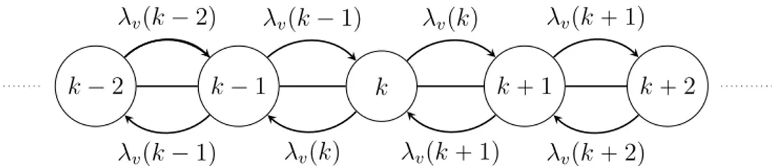
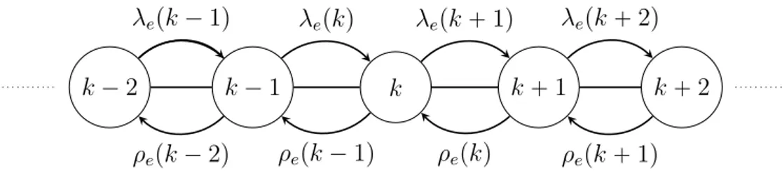
Using former results obtained by T.M. Liggett [52, 53], one obtains in Chapter 3 several survival and extinction conditions for the process. In that way, we consider two kinds of growth rates in Z : one where the rates depend on the edges and one where the rates depend on the vertices. This yields numerical bounds on the transitional phase for the process to survive or die out.

After having investigated the behaviour of each type of individuals in a microscopic scale, we now turn into the study of the system in a macroscopic scale. When the microscopic evolution is more intricate, by a suitable scaling in time and space, we investigate the convergence of the empirical densities of each type of population.

1.5.3 Hydrodynamic limit in a bounded domain

In Chapter 4, set S “ Td _{the d-dimensional torus, and assume the microscopic}

dy-namics is driven by the asymmetric multitype process pηtqtě0 along with a diffusion

process, modelling the migrations of the individuals. The diffusion process we consider here is a stirring process that exchanges two neighbouring occupation variables. Resul-ting with a reaction-diffusion process, we prove the convergence of the time-evolution of the empirical densities to the weak solution of a reaction-diffusion system.

(34)

1.5.4 Hydrodynamic limits with stochastic reservoirs or in

in-finite volume

One of the recurring reasons why the SIT fails, comes from an unexpected immi-gration in the system that prevents to maintain the pest population at a low level after regular releases. Such migrations with the external of the targeted area suggests the microscopic system is likely to be in non-equilibrium states.

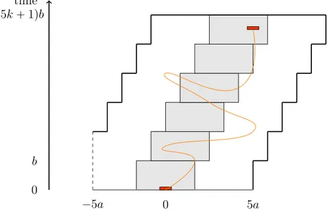
In Chapter 5, one considers the microscopic time-evolution to be driven by the CP-DRE along with a rapid-stirring process. We consider a bounded cylinder connected to stochastic reservoirs at its boundaries with different densities in a stationary regime, creating and annihilating individuals. Such reservoirs create a flow through the system that put it in a nonequilibrium state, as dynamics within the bulk is no more reversible. Jointly with M. Mourragui and E. Saada, we establish the limiting equations given by a non-linear reaction-diffusion system with Dirichlet boundary conditions and a law of large numbers for the empirical currents. In a second step, we derive the hydrodynamic limit of the CP-DRE with rapid-stirring in infinite volume Zd_.

(35)

(36)

2

Phase transition on the

d-dimensional integer lattice

2.1 Introduction

The Sterile insect technique concerns the control of a population by releasing sterile individuals of the same species, leading to a competition with the wild individuals to the reproduction. When a match with sterile individuals occurs, offsprings reach neither the adult phase nor sexual maturity, reducing the next generation.

This chapter is an attempt to understand the behaviour of the wild population with respect to the release of the competitive sterile individuals in this model. Following issues

(37)

corresponding to biology and ecology, a wide class of multi-type contact processes has emerged. Relevant questions are to identify the mechanisms involving survival, existence or coexistence of species ; such questions have been topics of works such as the grass-bushes-tree model by R. Durrett and G. Swindle [26], a 2-type contact process by C. Neuhauser [65], a 3-type model by R. Durrett and C. Neuhauser [23] for the spread of a plant disease.

The populations we consider are composed of wild males whereby sterile males are released at rate r to curb their development. We investigate the survival of the wild ones whose growth rate is time-evolving and randomly determined depending on the dynamics of the sterile individuals.

In Section 2.2, we describe the model and introduce some preliminary results about stochastic order and percolation. Then, we build graphically the particle system through Harris’ graphical representation in Section 2.3. After exhibiting necessary and sufficient conditions for monotonicity properties in Section 2.4, we prove the existence and uni-queness of a phase transition with respect to the release rate in Sections 2.5 and 2.6.

2.2 Settings and results

2.2.1 The model

On the state space Ω “ FS_{, where F “ t0, 1, 2, 3u and S “ Z}d_{, the multitype contact}

process is an interacting particle system pηtqtě0 whose configuration at time t is ηtP Ω,

that is, for all x P Zd_{, η}

tpxq P F represents the state of site x at time t. Two sites x and

y are nearest neighbours on Zd _{if }x ´ y} “ 1, also written x „ y, and n}

ipx, ηtq stands

for the number of nearest neighbours of x in state i, i “ 1, 3.

One understands the model as follows : at time t, a site x in Zd _{is empty if in state}

0, occupied by type-1 individuals if in state 1, by type-2 individuals if in state 2 and by both type-1 and type-2 individuals if in state 3.

Note that we only consider the type of individuals standing on each site and not their number. Moreover, we assume no limit on the number of female individuals, which is biologically a reasonable assumption (see Chapter 1).

Type-2 individuals act in two possible ways, they will reduce the growth rate of the type-1 individuals within sites in state 3. There, a competition occurs, so that the growth rate λ2 shall be lower than the regular growth rate λ1 in type-1 population where

stand only wild individuals. Our basic assumption is thus,

λ2 ă λ1. (2.2.1)

Furthermore, in a so-called asymmetric case, type-2 individuals will stem births on sites they occupy.

Since we deal with the evolution of a population modelled by a particle system, we will often mingle the terms “individuals” and “particles”.

(38)

The multitype contact process. Common transitions to both cases are the follo-wing : individuals on a site in state 1 (resp. 3) gives birth to type-1 individuals at rate

λ1 (resp. λ2) on one of its 2d nearest neighbour sites, if empty. A type-2 individual is

dropped independently and spontaneously at rate r on any site in Zd_{. Each type dies at}

rate 1, deaths are mutually independent. In the so-called symmetric case, births occurs on sites in state 2 as well.

Transition rates in x for a current configuration η that are common to both cases are : 0 Ñ 1 at rate λ1n1px, ηq ` λ2n3px, ηq 1 Ñ 0 at rate 1 0 Ñ 2 at rate r 2 Ñ 0 at rate 1 1 Ñ 3 at rate r 3 Ñ 1 at rate 1 3 Ñ 2 at rate 1 (2.2.2)

to which one adds the following transition in the symmetric case

2 Ñ 3 at rate λ1n1px, ηq ` λ2n3px, ηq. (2.2.3)

Therefore, the evolution of 2 individuals occurs whatever the evolution of type-1 individuals is. Since type-2 individuals dictate the growth rate and even inhibit births in the asymmetric case, the type-2 individuals shape a dynamic random environment for the type-1 individuals.

In both cases, if η P Ω and x P Zd, denote by η_xi P Ω, i P t0, 1, 2, 3u, the configuration obtained from η after a flip of x to state i :

η ÝÑ ηix at rate cpx, η, iq, where @u P Z d

, η_xipuq “" ηpuq if u ‰ x

i if u “ x (2.2.4)

Let L be the infinitesimal generator of pηtqtě0, then for any cylinder function f on Ω :

Lf pηq “ ÿ xPZd 3 ÿ i“0 cpx, η, iq`fpηixq ´ f pηq ˘ (2.2.5) with infinitesimal transition rates, common to both cases,

cpx, η, 0q “ 1 if ηpxq P t1, 2u cpx, η, 1q “" λ1n1px, ηq ` λ2n3px, ηq if ηpxq “ 0 1 if ηpxq “ 3 cpx, η, 2q “" r if ηpxq “ 0 1 if ηpxq “ 3 cpx, η, 3q “ r if ηpxq “ 1 (2.2.6)

(39)

and add the following rate in the symmetric case :

cpx, η, 3q “ λ1n1px, ηq ` λ2n3px, ηq if ηpxq “ 2.

Notice that all rates satisfy for all i P F ,

cpx, η, iq ě 0, sup x,η cpx, η, iq ă 8, (2.2.7) sup xPZd ř uPZd sup η |cpx, ηu, iq ´ cpx, η, iq| ă 8. (2.2.8)

Under these mild conditions, by Theorem 1.1.3 there exists a unique Markov process associated to the generator (2.2.5). Denote by pηA

t qtě0 the process starting from A, i.e.

such that η0 “ 1A, in other words η0 corresponds to the configuration containing sites in

state 1 in A and empty otherwise. We care about the evolution of the wild population, i.e. individuals contained in sites in state 1 and 3. Define

H_tA“ tx P Zd : η_tApxq P t1, 3uu, (2.2.9) as the set of sites containing the wild population at time t ě 0. Note that since η0 “ t0u,

H₀t0u “ tx P Zd : η₀t0upxq “ 1u.

Denote by Pλ1,λ2,r the distribution of pη

t0u

t qtě0 with parameters pλ1, λ2, rq. For fixed

λ1 and λ2, simplify by Pr.

Definition 2.2.1. The process pηtqtě0 with initial configuration η0 “ 1t0u, survives if

Pλ1,λ2,rp@t ě 0, H

t0u

t ‰ Hq ą 0 (2.2.10)

and dies out if

Pλ1,λ2,rpDt ě 0, H

t0u

t “ Hq “ 1. (2.2.11)

Define the critical value according to the parameter r by

rc“ rcpλ1, λ2q :“ inftr ą 0 : PrpDt ě 0, H t0u

t “ Hq “ 1u (2.2.12)

Indeed, the class t0, 2u is a trap : as soon as Ht “ H, the wild population is extinct

while sterile individuals are constantly dropped along the time.

Recall λc stands for the critical value of the basic contact process. The purpose of

this chapter is to settle the following results.

We begin by a first set of conditions for the process to survive or die out, when

λ2 ă λ1 are both smaller or larger than λc :

Proposition 2.2.1. Suppose λ2 ă λ1 ď λc. For all r ě 0, both symmetric and