UNIVERSIT ´E DU QU ´EBEC `A RIMOUSKI
HYDRODYNAMIQUE DE LA BAIE DE SEPT-ˆILES
M ´EMOIRE PR ´ESENT ´E
dans le cadre du programme de maˆıtrise en oc´eanographie en vue de l’obtention du grade de M. Sc.
PAR
©JEAN-LUC SHAW
Composition du jury :
C´edric Chavanne, pr´esident du jury, Universit´e du Qu´ebec `a Rimouski
Daniel Bourgault, directeur de recherche, Universit´e du Qu´ebec `a Rimouski
Dany Dumont, codirecteur de recherche, Universit´e du Qu´ebec `a Rimouski
Fr´ed´eric Cyr, examinateur externe, Pˆeches et Oc´eans Canada
UNIVERSIT ´E DU QU ´EBEC `A RIMOUSKI Service de la biblioth`eque
Avertissement
La diffusion de ce m´emoire ou de cette th`ese se fait dans le respect des droits de son auteur, qui a sign´e le formulaire Autorisation de reproduire et de diffuser un rapport, un m´emoire
ou une th`ese . En signant ce formulaire, l’auteur conc`ede `a l’Universit´e du Qu´ebec `a
Ri-mouski une licence non exclusive d’utilisation et de publication de la totalit´e ou d’une par-tie importante de son travail de recherche pour des fins p´edagogiques et non commerciales. Plus pr´ecis´ement, l’auteur autorise l’Universit´e du Qu´ebec `a Rimouski `a reproduire, diffuser, prˆeter, distribuer ou vendre des copies de son travail de recherche `a des fins non commer-ciales sur quelque support que ce soit, y compris l’Internet. Cette licence et cette autorisation n’entraˆınent pas une renonciation de la part de l’auteur `a ses droits moraux ni `a ses droits de propri´et´e intellectuelle. Sauf entente contraire, l’auteur conserve la libert´e de diffuser et de commercialiser ou non ce travail dont il poss`ede un exemplaire.
Il continue `a fixer la mer. Silence. De temps en temps, il trempe le pinceau dans une tasse de cuivre et trace sur la toile quelques traits l´egers. Les soies du pinceau laissent derri`ere elles l’ombre d’une ombre tr`es pˆale que le vent s`eche aussitˆot en ramenant la blancheur d’avant. De l’eau. Dans la tasse de cuivre il n’y a que de l’eau.
- Extrait de Oc´ean mer, Alessandro Baricco
REMERCIEMENTS
Ce projet n’aurait pas ´et´e possible sans l’aide d’un longue liste de personnes. Je tiens `a remercier tous ceux qui nous ont aid´e sur le terrain, Simon B´elanger, Carlos Ara´ujo, Alexandre Th´eberge, Aur´elie Le H´enaff, Bruno Saint-Denis, Jean-Franc¸ois Beaudoin, Kim Aubut-Demers et Z´elie Schuhmacher. Julie Carri`ere et Laurence Paquette ont aussi fourni une aide indispen-sable dans la gestion de la logistique. J’offre ´egalement mes remerciements aux capitaines Alain Saint-Pierre, Glenn Galichon et Jean Philippe Blouin. Sans eux, nos mesures en mer n’auraient pas ´et´e possibles.
Mes directeurs Daniel et Dany sont aussi m´eritants de remerciements sinc`eres. Tout en offrant un encadrement solide `a mon projet, vous avez laiss´e beaucoup de place `a mes initiatives. Les comp´etences que j’ai d´evelopp´ees en les poursuivant ont sans doute contribu´e `a lancer ma carri`ere professionnelle. J’appr´ecie `a quel point vous avez ´et´e disponibles tout au long de mon projet. J’ai toujours eu r´eponse satisfaisante `a mes questions au moment o`u j’en avais besoin. Je vous remercie aussi de m’avoir invit´e `a participer `a vos projets de recherche respectifs. Que ce soit pour regarder l’eau du Saguenay du haut d’une montagne ou cirer un canot `a glace, ces invitations ont grandement enrichi mon exp´erience ´etudiante et mon bagage professionnel ! Votre critique de mon travail a toujours ´et´e p´edagogique et constructive. Par elle vous, m’avez pouss´e `a me d´epasser et `a produire un m´emoire dont je suis fier. J’´etends d’ailleurs ma gratitude autres membres de mon comit´e d’´evaluation, C´edric Chavanne et Fr´ed´eric Cyr, qui ont accept´e de le lire.
Enfin, je souhaite remercier les gens qui m’ont soutenu par leur pr´esence et leur amiti´e. `
A mes camarades de bureau Bruno, Jean, Jean-Franc¸ois, Karine, Kevin, Michel et S´ebastien, c¸a ´et´e un plaisir de partager le quotidien de mon projet avec vous, dans tous ses petits succ`es et ses p´epins. `A mes amis dans les autres bureaux, Ariane, Aude, Constance, Fatma, Jor-dan, Laurie-Emma, Omnain, Safwen, Sarah, Simon, Sophia et Yan, on se sera pas vus assez souvent ! `A mes colocs de la maison brune, Annabelle, Marianne, Marie- `Eve, Fred, Geoffroy,
viii
Simon et Chamou, vous avez rempli chaque jour de chaleur, de douceur, de rire et d’aventure. Je vous en remercie du fond du coeur. `A Florence, tu en sais probablement beaucoup plus sur la baie de Sept-ˆIles que ce que ton int´erˆet motive ! Je te remercie de m’avoir ´ecout´e avec patience. Je te remercie aussi d’avoir ´et´e une partenaire ind´efectible pendant ma maˆıtrise et d’avoir vaillamment endur´e trois ans de relation `a distance pour que ton copain aille `a l’´ecole.
R ´ESUM ´E
Les variabilit´es tidale et saisonni`ere de la temp´erature, la salinit´e et les courants ont ´et´e mesur´ees dans la baie de Sept-ˆIles (BSI) du printemps `a l’automne 2017 et au printemps 2018. Des bou´ees d´erivantes et des profileurs ADCP ont ´et´e d´eploy´es pour mesurer les courants et des profils CTDs ont ´et´e r´ecolt´es 5 fois `a 21 stations r´eparties dans la baie et l’archipel. Des passages r´ep´et´es pendant 12 h le long d’un transect `a l’embouchure ont ´et´e r´ealis´es avec un ADCP en route. Durant cette mesure, des arrˆets r´eguliers ont ´et´e faits pour collecter des profils CTDs. Les courants moyenn´es sur un cycle de mar´ee ´etaient vers l’aval pr`es de la surface (0-5 m) et g´en´eralement vers l’amont en eau plus profonde (1(0-5-(0-50 m). Un courant vers l’aval a ´et´e mesur´e pr`es de Pointe `a la Marmite tout au long du cycle de mar´ee et apparaˆıt aussi dans les donn´ees de bou´ees d´erivantes. Les vitesses moyennes et maximales de bou´ees d´erivantes sont de 17.4 cm s−1et 86.6 cm s−1. Leur cap ´etait en moyenne 24±39◦ `a l’ouest du cap du vent et elles se sont ´echou´ees sur les plages oppos´ees aux directions des vents dominants (NNW et ESE) dans 22/46 des cas. Un courant anti-cyclonique `a l’´echelle de la baie a ´et´e mesur´e `a mar´ee montante et la circulation de surface ´etait cyclonique en moyenne pr`es de la surface au jusant. La perturbation saisonni`ere de stratification ´etait `a son plus fort au d´ebut du mois de juin et son influence ´etait surtout sentie dans les 20 m sous la surface. Le temps de r´esidence de la BSI est estim´e entre 2-12 jours. Le rayon interne de Rossby est calcul´e `a LD= 2.8 km et
LD= 6.8 km en stratification respectivement faible et forte, sugg´erant que l’effet de la rotation
de la terre sur l’hydrodynamique ne peut pas ˆetre n´eglig´e. Une critique du mod`ele conceptuel existant de la circulation dans la BSI est ´emise, ainsi que des recommandations en vue d’un nouveau mod`ele.
ABSTRACT
Seasonal and tidal variability of temperature, salinity, and currents were measured in the bay of Sept-ˆIles (BSI) from spring to fall 2017, and in spring 2018. Surface drifters and ADCP profilers were deployed to measure current velocities and CTD profiles were recorded regularly at 21 stations spread out across the bay and archipelago. Repeated passages along a transect at the bay mouth were conducted during 12 hours with an underway ADCP. During these transects, regular stops were made for CTD profiling. Tidally-averaged currents were out-flowing near the surface (0-5 m) and generally in-flowing in deeper waters (15-50 m). A seaward current was measured near Pointe `a la Marmite throughout the tidal cycle and also appears in drifter data. Surface drifter speeds average to 17.4 cm s−1but reached up to 86.6 cm s−1. Drifter heading was 24±39◦west of wind direction on average and they shoaled
on beaches leeward of dominant winds (NNW and ESE) in 22/46 cases. A bay scale anti-cyclonic current was measured at rising tide and surface circulation during ebb was anti-cyclonic on average. Seasonal disturbance of stratification was strongest in early June and was mostly felt in the top 20 meters. Bulk residence time for water in the BSI is scaled to 2-12 days. The internal Rossby radius is scaled to LD = 2.8 km and LD= 6.8 km during low and high
stratification, suggesting influence of earth’s rotation on hydrodynamics can not be neglected. Criticism of the existing conceptual model for circulation in the BSI, and a starting point for a new model are given.
TABLE DES MATI `ERES
REMERCIEMENTS . . . vii
R ´ESUM ´E . . . ix
ABSTRACT . . . x
TABLE DES MATI `ERES . . . xi
LISTE DES TABLEAUX . . . xiii
LISTE DES FIGURES . . . xiv
INTRODUCTION G ´EN ´ERALE . . . 2
ARTICLE I HYDRODYNAMICS OF THE BAY OF SEPT-ˆILES . . . 9
1.1 Abstract . . . 9
1.2 Introduction . . . 10
1.3 Datasets and Methodology . . . 14
1.3.1 Sampling . . . 14
1.3.2 Third party data . . . 17
1.3.3 Processing . . . 17
1.3.4 Problems encountered . . . 23
1.4 Results . . . 24
1.4.1 Harmonic analysis of tides . . . 24
1.4.2 Wind statistics . . . 25
1.4.3 Temporal variability . . . 27
1.4.4 Spatial variability . . . 43
1.5 Discussion . . . 49
1.5.1 Influence of Earth’s rotation . . . 49
1.5.2 Fresh water input . . . 50
1.5.3 Flushing time . . . 51
1.5.4 Current forcing . . . 53
xii 1.6 Conclusion . . . 56 1.7 Acknowledgments . . . 58 CONCLUSION G ´EN ´ERALE . . . 59 R ´EF ´ERENCES . . . 64 ANNEXE A ADCP COMPASS CORRECTION SCHEMES . . . 67
LISTE DES TABLEAUX
1 Sommaire des dates et op´erations de collecte de donn´ees. . . 7 2 Summary of sampling dates and data sets collected. . . 15 3 Name, period, amplitude, energy percentage, and Greenwich phase lag of 10
main tidal constituents, sorted by decreasing energy. . . 24
4 N2
max (10−3 s−2) for the profiles along T3 at different times of the season.
Columns indicate distance from the station furthest offshore. . . 28 5 Average temperature and practical salinity shown with standard deviation for
the top 10 m hS , T is, and for the 10 to 30-m layer hS , T ib. . . 30
6 Temperature and salinity difference between the south, center and north sam-pling stations for the reconstructed tide cycles of June 2017 (top row), Sep-tember 2017 (middle row), and May 2018 (bottom row). The left column indicates tidal phase in hours after high tide. . . 34 7 Profile maximum buoyancy frequency south, center, and north of T1, with
corresponding depth. The left column shows time after high tide. The top, middle and bottom tiers show June 2017, September 2017, and May 2018 measurements, respectively. . . 36
8 Summary of underway ADCP measurement parameters. All measurements used a Teledyne RDI Sentinel V 500 kHz profiler. Measurement from 21/06/2017 is not shown here. It was conducted in the shallow parts of the bay following the shore in the clockwise direction. . . 67
LISTE DES FIGURES
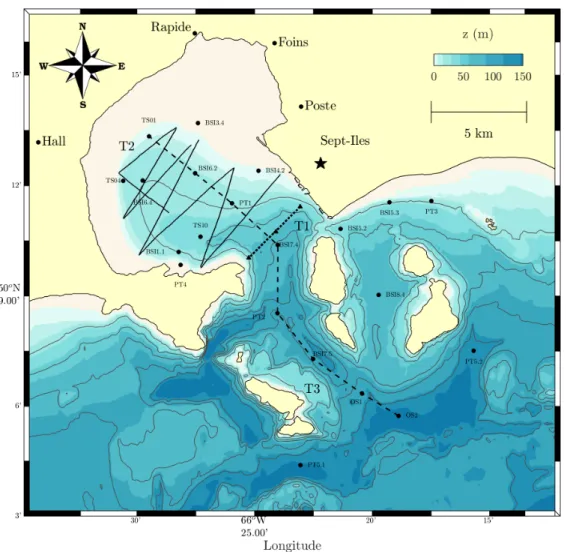
1 G´eographie des mesures courantologiques effectu´ees dans la BSI par des ´etudes pr´ec´edentes. Les symboles marquent des mouillages et les lignes des transects d’ADCP en route. . . 4 2 Regular sampling stations (•) and transects. Stations marked byN only
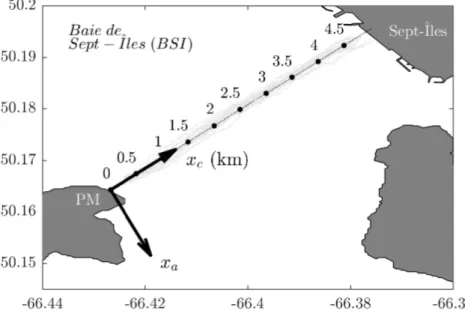
sam-pled during 12 h repeated transects. The locations on land are the bridges from which the rivers were sampled. T1 (dotted) and T2 (solid) correspond to underway ADCP transects. T3 (dashed) is the main CTD transect. Bathy-metric contours are 5 meters apart. Solid contours mark 25 m intervals. . . 11 3 Definition of coordinates xc and xaalong transect T1. . . 18
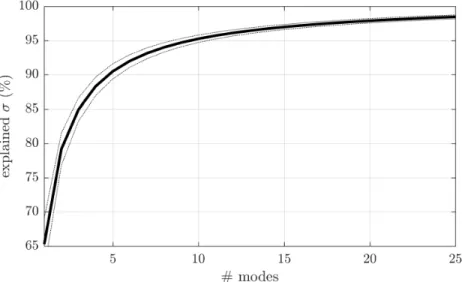
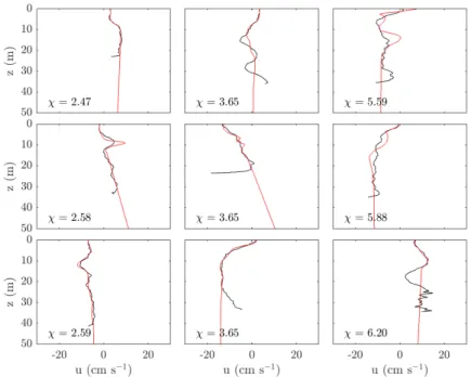
4 Percentage of ADCP profile variance explained as a function of the number of vertical modes considered. The solid line shows the average over all profiles and the envelope is standard deviation. . . 21 5 Eastward velocity from ADCP data (black) and adjusted current profile (red)
for the three best fits (left), three average fits (center), and the three worst fits (right). Associated χ (cm s−1) values are written in the bottom left. . . . 22
6 Wind provenance from the HRDPS wind model. Panel a) shows data from Febuary 2017 to Febuary 2018. Panel b) shows data from April 2017 to No-vember 2017. Panel c) shows data from NoNo-vember 2017 to April 2018. . . 26 7 Seasonal change in temperature (top) and salinity (bottom) along transect
T3. Distance along T3 with 0 at the offshore station is on the x axis. Date of sampling is written in the bottom right corner of each panel. . . 29 8 Temperature and salinity data and it’s seasonal variability. Marker shape
in-dicates sampling campaign and depth is shown by the color axis. ’*’ symbols in the legend mark sampling campaigns where only a subset of stations are visited. Salinities as low as 16.52 where measured but only in the 06/06 cam-paign and are not shown for clarity. Boxes are centered on the surface 10 meter mean values (see Table 5) for each campaign and are 2 standard devia-tions wide in both direcdevia-tions. . . 31 9 Evolution of the average water column density structure through the season.
The color axis shows density, whereas the overlaid solid black lines show temperature. Standard deviation between stations is computed for every cam-paign and shown on the left. Dashed lines indicate times of sampling camcam-paigns. 32
xv
10 Time series of river discharge for three rivers, Rapide (local), Moisie (regio-nal), and St. Lawrence (large scale). The area between climatological maxi-mums and minimaxi-mums is shown in grey. For the middle and bottom panels the solid black line shows 2017 values. Since these values are unavailable for rivi`ere des Rapides, the climatology mean is shown. Dashed lines indicate times of sampling campaigns. Top two panels made from CEHQ tide gauge data, and bottom panel shows RIVSUM. . . 33 11 Reconstructed temperature (color) and salinity (solid lines) fields along T1.
Columns are June 2017 (left), September 2017 (center), and May 2018 (right) repeated transects. Rows are approximately corresponding tidal phase, as is written in hours after high tide. Note the different color axes for each column. 35 12 Reconstructed reduced stratification and salinity fields at four tidal phases
noted by the inset. Solid lines show salinity while colored contours show reduced stratification. Data inside the yellow line is from measurements and data outside uses extrapolation. Nr2is smoothed vertically using a 4 m moving
average and a 1.5 hour moving average in time. . . 38 13 Reconstructed tidal cycle from repeated transects. Vector colors show
repre-sented depth layer. Tidal phase is found on the inset. Data is passed through a 3 hour moving time average. Gray arrow shows average cross transect current direction in the unmeasured area, norm is written in matching color. . . 39 14 Along shore velocity averaged over 12.5 hours. Speed values inside the
yel-low contours are from measurements. . . 40 15 Maximum cross shore velocity estimate during spring tide (amplitude= 1.755
m) shown by the color axis. Overlaid black coutours are bathymetry. . . 42 16 Drifter tracks and their box averaged speeds. Ellipses follow the same scale
as arrows and show standard deviation in the two principal axes of variation. Dots and crosses show deployment and last ping respectively. Blue tracks are the DFO measurements from 2003, red tracks are purposely put at the mouth of rivers, and black tracks are ship borne deployments. Numbers are cumula-tive hours of drift per box. Left and right bottom panels are box averages for ebb and flood data. . . 44 17 Probability density distribution for speed amplitudes of all drifter data
recor-ded north of 50.05◦(top), T1 ADCP data in first 9 m (middle), and the rest of the water column (bottom). Average values are shown by the dashed line. . . 46
xvi
18 Toroidal projection of drifter heading θd plotted against wind heading θw
(0◦=E, 90◦=N) interpolated in time and space. Black dots indicate the
ori-gins of axes θd and θw, respectively running counter clockwise, and from the
inside out. The color axis highlights corresponding wind speed and the solid black line marks the 1 :1 ratio. . . 47 19 Interpolated synoptic image of ADCP measurements inside the bay. On the
top panel, time of sampling is highlighted in black over the sea surface ele-vation curve, and wind feather plot. Mean wind vectors during these measu-rements are shown on the bottom left. The second, third and last panels from the top show mean surface layer speeds, bottom layer speeds, and depth ave-raged vertical velocity (positive downwards) respectively. Vector colors note the day of measurement, ship track is shown by the dashed line and the color axis shows temperature (second panel), depth (third panel), and w (bottom panel). . . 48 20 The Roche (2000) conceptual model for a) ebb and b) flood currents, and c)
our proposed schematic synthesis of the observed BSI circulation. North is towards the top of the page in a) and b). In c) the bottom layer follows the east-west axis. Red, blue and gray arrows stand for ebb, flood and tidally ave-raged currents. Full arrows designate averages from one or more tidal cycles. Dashed arrows represent an assessment made from a single measurement. . . 54
21 Comparison between speed deduced from the track log of 17/05/2018 and the opposite of bottom track velocities. . . 69 22 Stick plot time series of the opposite of the raw bottom track velocity (top),
rotated bottom track (middle), and GPS velocities (bottom). The north ve-locity component points upwards and the eastward component points to the right. The section when the ADCP was used as a heading source is circled. . 70 23 Measured ADCP along shore (top) and cross shore (bottom) velocities for
the May 17 2018 transects. The left panels are raw, while the right have been rotated by∆θ. Ship track is shown by the dotted line. . . 71 24 Statistical (top) and time series (bottom) representation of the difference
be-tween θp and θbfor the repeated transects of June 20 (left) and September 25
(right), 2017. . . 72 25 Measured ADCP along shore (top) and cross shore (bottom) velocities for the
May (left) and September (right) transects. Ship track is shown by the dotted line. . . 73
INTRODUCTION G ´EN ´ERALE
Motivation
L’´evaluation objective de la sant´e d’un ´ecosyst`eme peut s’av`erer une tˆache complexe, surtout en pr´esence d’un biˆome richement diversifi´e comme on en trouve souvent dans les baies (Greenlaw et al., 2011). Pour surveiller la sant´e globale des ´ecosyst`emes en ne consid´erant qu’un sous-ensemble fini de leurs param`etres, des indices de sant´e ´ecologiques sont d´evelopp´es notamment en Europe (Birk et al., 2012) et dans une vari´et´e d’endroits (Halpern et al., 2008), visant une application locale.
L’indice de sant´e des oc´eans (OHI) d´evelopp´e par Halpern et al. (2012) est un exemple de ces m´ethodes. Afin de chiffrer la sant´e d’un ´ecosyst`eme, sa r´eponse aux stress anthropique, biologique et climatique est d’abord utilis´ee pour pr´edire son ´etat futur. Une comparaison entre cet ´etat futur et un ´etat de r´ef´erence sain ´evalue son ´etat de sant´e pr´esent. Il est toutefois connu que les indices de sant´e ´ecologiques sont peu fiables `a l’ext´erieur des ´ecosyst`emes pour lesquels ils ont ´et´e d´evelopp´es (Gillett et al., 2015).
En contexte d’une pr´esence humaine croissante aux latitudes arctiques et sub-arctiques, il y a aussi un besoin croissant de d´evelopper des outils pour aider les d´ecideurs `a g´erer de fac¸on durable et inform´ee par la science. Pour r´epondre `a ce besoin, une ´etude multi-disciplinaire a ´et´e conduite dans le cadre du partenariat strat´egique Canadian Healthy Oceans Network (CHONe) en collaboration avec l’Institut nordique de recherche en environnement en sant´e au travail (INREST) visant `a d´evelopper un indice de sant´e ´ecologique adapt´e `a la baie de Sept-ˆIles (BSI).
3
Objectifs
Les diff´erents facteurs de stress qui agissent sur la sant´e d’un ´ecosyst`eme le font d’une fac¸on hautement interactive, c’est pourquoi une approche int´egratrice des param`etres chi-miques, biologiques et physiques est `a favoriser (Halpern et al., 2012). Vecteur de transport de tous les param`etres physico-chimiques marins, la circulation de l’eau est un ´el´ement cl´e de la dynamique de ces interactions. Elle peut notamment ´evacuer, retenir, concentrer ou importer des contributions au stress anthropique. Une compr´ehension quantitative de l’hy-drodynamique de la BSI est une ´etape incontournable `a franchir en vue de d´evelopper des indicateurs ´ecologiques performants pour cette aire d’´etude. L’objectif de ce projet est de construire un jeu de donn´ees suffisant pour r´esoudre et quantifier dans la BSI la variabilit´e des param`etres physiques `a l’´echelle tidale et saisonni`ere, et pour permettre la validation et calibration de mod`eles hydrodynamiques.
La baie de Sept-ˆIles
Fortement industrialis´ee et sujette `a un traffic maritime international, la BSI se trouve `a proximit´e d’´ecosyt`emes semblables (Baie Sainte-Marguerite, Baie Moisie) qui sont moins sujets `a l’influence humaine, faisant de ce locus un endroit pratique pour ´etudier l’effet du stress anthropique sur les communaut´es benthiques et p´elagiques en climat sub-arctique.
La BSI (figure 1) est situ´ee dans le nord-ouest du golfe du Saint-Laurent (GSL) `a 50◦N. Une comparaison entre la largeur de son embouchure (5 km) et son plus long diam`etre (13 km) la classifie comme une baie renferm´ee. `A 2.3 m et 3.7 m de marnage pour les mar´ees moyennes et les grandes mar´ees (Proc´ean, 1999), la BSI serait consid´er´ee comme un estuaire m´esotidal par Dyer (1973). `A l’int´erieur du transect T1 (figure 2) la baie contient environ 1.1 km3 d’eau et s’´etend sur 100 km2. De cette superficie, les profondeurs inf´erieures et sup´erieures `a 30 m repr´esentent respectivement 58% et 11%. Le reste repr´esente la zone
in-4
Figure 1: G´eographie des mesures courantologiques effectu´ees dans la BSI par des ´etudes pr´ec´edentes. Les symboles marquent des mouillages et les lignes des transects d’ADCP en route.
tertidale le long des berges. La profondeur maximale `a l’embouchure est de 72 m et vers l’aval, la profondeur augmente parfois au-del`a de 100 m pour former les passages entre les six ˆıles et la presqu’ˆıle qui donnent `a la baie son nom. Les rivi`eres Hall, aux Foins, du Poste et des Rapides se d´eversent dans la baie en provenance d’un bassin versant dont la superficie est 788 km2. Elles apportent 22 m3s−1d’eau douce en moyenne annuellement (Proc´ean, 1999).
Il existe certaines ´etudes d´ecrivant des mesures hydrodynamiques dans la BSI, mais leur couverture spatiale ou temporelle est souvent tr`es locale. La r´epartition g´eographique des mesures courantologiques r´ecolt´ees pour ces ´etudes est pr´esent´ee `a la Figure 1. Une d´erive
5
littorale vers l’ouest est propos´ee par Hein et al. (1993) pour expliquer l’´evolution moderne des d´epˆots de m´etaux lourds sur le delta de la rivi`ere Moisie, `a l’est de Sept-ˆIles. Des couran-tom`etres ont ´et´e plac´es `a l’embouchure de la rivi`ere Moisie par Koutitonsky and Long (1991) qui ont enregistr´e des vitesses instantan´ees de l’ordre de 20 cm s−1, globalement orient´ees le long des berges vers le sud-ouest. Ils ont aussi enregistr´e des vitesses allant jusqu’`a 1.5 m s−1 durant les tempˆetes et not´e la corr´elation de ces vitesses avec la hauteur de la houle. Deux courantom`etres ont ´et´e mouill´es par Neumeier and Joly (2014) `a environ 10 km `a l’est de la BSI de 2010 `a 2014. L’un ´etait pr`es de la cˆote `a une profondeur de 4.4 m alors que le second ´etait `a 4.5 km de la cˆote `a 28 m de profondeur. Il ont trouv´e que les courants dans cette zone s’´ecoulaient g´en´eralement le long des cˆotes et changeaient de direction selon les mar´ees, mais sont dominants vers l’ouest lorsque moyenn´es sur 4 ans `a l’exception des courants de surface au mouillage profond qui sont dominants vers l’est. `A l’int´erieur de la baie, Roche (1991) (consult´e dans Belles-Isles et al. 2003) d´ecrivent des courants qui longent les berges, mais dont la direction change avec les mar´ees pr`es de la ville de Sept-ˆIles. L’´etude la plus exhaus-tive `a ce jour a ´et´e men´ee par Proc´ean (1999) qui emploie deux mouillages ´equip´es de cou-rantom`etres acoustiques (ADCP) plac´es dans la portion sud de la baie, ainsi que des transects d’ADCP en route r´ep´et´es pendant un ou deux cycles de mar´ee `a trois endroits diff´erents. Leur mouillage le plus profond (S1) signale des courants plus forts en profondeur (0-35 cm s−1) qu’`a mi-profondeur (0-17 cm s−1) et dirig´es vers 290◦ou 135◦, selon les mar´ees. Ils d´etaillent les courants `a l’embouchure `a mar´ee haute, mar´ee basse, au jusant et au flot tel que mesur´es par leur ADCP en route. En surface, ils trouvent des vitesses vers l’amont `a toutes les phases de mar´ee sauf le jusant. Les vitesses maximales (∼42 cm s−1) y sont mesur´ees en p´eriode de flot. Au jusant, les courants de surface sont mesur´es vers l’aval `a l’exception d’un courant vers l’amont mesur´e pr`es de Pointe `a la Marmite. En profondeur, ils mesurent des courants plus faibles (< 20 cm s−1) et plus spatialement variables qui s’´ecoulent vers l’aval. Des courants encore plus faibles (< 10 cm s−1) sont toutefois mesur´es vers l’amont pour ces profondeurs
`a plusieurs phases de mar´ee. Les transects r´ep´et´es `a l’int´erieur de la baie ont montr´e jusqu’`a quatre couches de courants cisaill´es que Roche (2000) interpr`ete comme des cellules
verti-6
cales forc´ees par le vent telles qu’on en retrouve dans les mod`eles physiques de lacs stratifi´es (Hutter et al., 2011). Roche (2000) ont aussi mouill´e des courantom`etres dans la portion sud de la BSI pendant 66 jours. Ils ont mesur´e des courants allant jusqu’`a 40 cm s−1et longeant principalement la cˆote. Une analyse de vecteur progressif pour ces donn´ees montre une vi-tesse r´esiduelle vers l’est dans cette r´egion. Leur rapport pr´esente ´egalement des profils de conductivit´e, temp´erature et profondeur (CTD) provenant de plusieurs endroits dans la BSI montrant une stratification `a deux couches dont celle de surface (0-15 m) ´etait caract´eris´ee par des temp´eratures et salinit´es de ∼10◦C et ∼30 PSU, alors que ∼4◦C et ∼31 PSU sont mesur´es en couche de fond le 6 aoˆut 1999. `A partir de ces donn´ees, ils proposent un mod`ele concep-tuel pour la circulation dans la BSI dont la forme est repr´esent´ee par un r´eservoir circulaire avec une entr´ee d’eau orient´ee vers le nord connect´ee `a son extr´emit´e est. Ils consid`erent que la circulation est cyclonique lorsque l’eau entre dans le r´eservoir et anti-cyclonique conver-gente vers l’entr´ee lorsque l’eau en est retir´ee. Aucune mesure, simulation ou r´ef´erence n’est toutefois pr´esent´ee en appui `a ces affirmations. Si leurs donn´ees de mouillage et leur mod`ele conceptuel sont en accord, les donn´ees sont tr`es localis´ees. Leurs mouillages ´etaient `a 1 km de s´eparation le long de l’isobath 10 m, `a environ 0.5 km de la berge sud. Aucune donn´ee n’est pr´esent´ee qui permet d’´evaluer la validit´e du mod`ele conceptuel ailleurs dans la BSI.
M´ethodologie
La visite de 21 stations r´eparties dans la baie et l’archipel pour y r´ecolter des profils de temp´erature, salinit´e et courants, r´ep´et´ee `a 5 reprises au cours de l’´et´e 2017 (tableau 1) constituait le coeur de l’´echantillonnage de ce projet de recherche. Le transect T1 (figure 2) `a l’embouchure de la baie a aussi ´et´e choisi pour explorer la variabilit´e tidale de la BSI. Des passages r´ep´et´es ont ´et´e r´ealis´es en le longeant durant un cycle de mar´ee semi-diurne (12 h), r´ecoltant des profils de courantom`etre acoustique `a effet doppler (ADCP) en continu et des profils CTD lors d’un passage sur trois. Des bou´ees d´erivantes munies de balises GPS ont aussi ´et´e d´eploy´ees lors des transits afin de r´ecolter de l’information sur les courants de
7
surface. Toutes les donn´ees de 2017 ont ´et´e collect´ees `a bord du navire de pˆeche au crabe le Yvan-Raymond, `a l’exception d’un d´eploiement de bou´ees le 26 septembre effectu´e `a partir d’un plus petit navire, le Monica. Les mesures d’ADCP en route collect´ees en mai 2018 le long des transects T1 et T2 (voir figure 2) ont ´et´e collect´ees `a bord du navire F. J. Saucier appartenant au Centre interdisciplinaire de recherche en cartographie des oc´eans (CIDCO).
Dates (dd/mm/yyyy) Stations CTD Stations ADCP Bou´ees ADCP en route CTD T1
04-06/05/2017 × × × 21-22/05/2017 × 06-07/06/2017 × × × 19-23/06/2017 × × × × × 24-26/09/2017 × × × × × 15-18/05/2018 × × ×
Table 1: Sommaire des dates et op´erations de collecte de donn´ees.
Une pleine compr´ehension de l’hydrodynamique d’un bassin comme la BSI est difficile `a atteindre sans avoir recours `a la mod´elisation. Les travaux pr´esent´es ici visent n´eanmoins `a en produire une description aussi d´etaill´ee que le permettent les observation recueillies.
`
A cette fin, un portrait des conditions de vent (section 1.4.2), des mar´ees (section 1.4.1) et du d´ebit des tributaires a d’abord ´et´e dress´e `a l’aide de donn´ees obtenues d’Environnement et changement climatique Canada (ECCC), du Service hydrographique du Canada (SHC) et du Centre d’expertise hydrique du Qu´ebec (CEHQ). Un large ´eventail d’analyses int´egrant ces donn´ees contextuelles avec les donn´ees nouvellement acquises ont ensuite ´et´e effectu´ees pour en d´egager les tendances tidales et saisonni`eres d´ecrites `a la section 1.4.3, ainsi que les tendances spatiales d´ecrites `a la section 1.4.4. Ces r´esultats ont permis de proposer une compr´ehension pr´eliminaire de la circulation dans la BSI synth´etis´ee aux sections 1.5.4 et 1.5.5. Ils ont aussi permis d’avancer des recommandations d’exp´eriences `a conduire advenant qu’une ´etude de mod´elisation num´erique soit r´ealis´ee.
ARTICLE I
HYDRODYNAMICS OF THE BAY OF SEPT-ˆILES
1.1 Abstract
Seasonal and tidal variability of temperature, salinity, and currents were measured in the bay of Sept-ˆIles from spring to fall 2017, and in spring 2018. Surface drifters and ADCP profilers were deployed to measure current velocities and CTD profiles were recorded reg-ularly at 21 stations spread out across the bay and archipelago. Repeated passages along a transect at the bay mouth were conducted during 12 hours with an underway ADCP. During these transects, regular stops were made for CTD profiling. Seasonal disturbance of stratifi-cation was strongest in early June and was mostly felt in the top 20 meters. Tidally-averaged currents were out-flowing near the surface (0-5 m) and generally in-flowing in deeper waters (15-50 m). A seaward current was measured near Pointe `a la Marmite throughout the tidal cy-cle and also appears in drifter data. Surface drifter speeds average to 17.4 cm s−1but reached up to 86.6 cm s−1. Drifter heading was 24±39◦ west of wind direction on average and they shoaled on beaches opposing dominant wind directions (NNW and ESE) in 22/46 cases. A bay scale anti-cyclonic current was measured at rising tide and surface circulation during ebb was cyclonic on average. Bulk residence time for water in the BSI is scaled to 2-12 days. The internal Rossby radius is scaled to LD= 2.8 and LD = 6.8 during low and high stratification,
suggesting influence of earth’s rotation on hydrodynamics can not be neglected. Criticism of the existing conceptual model for circulation in the BSI, and a starting point for a new model are given.
10
1.2 Introduction
Objective evaluation of the health of an ecosystem can prove to be a complex task especially in the presence of a richly diverse biota, such as is often found in bay environments (Greenlaw et al., 2011). In an effort to monitor the global health state of ecosystems using a finite set of parameters, ecological indicators have developed notably in Europe (Birk et al., 2012), and in various places (Halpern et al., 2008), designed for local application.
The Ocean Health Index (OHI) developed by Halpern et al. (2012) exemplifies this method. To produce an ecosystem’s score according to its framework, response of an ecosys-tem to anthropogenic, biological and climatic stress factors is used to predict its future state. Comparison of this future state with a reference healthy state determines the ecosystem’s health score. However, it is a known caveat that ecological indicators are often unreliable outside the ecosystem for which they were designed (Gillett et al., 2015).
In the context of growing anthropic presence at sub-arctic and arctic latitudes, there is a corresponding growing need for the development of tools to help managers make sustainable and science-based decisions. To answer this need, a multidisciplinary study was conducted by the Canadian Healthy Oceans Network (CHONe) strategic partnership in collaboration with the Nordic institute of research in environment and health in the workplace (INREST) aiming at designing ecosystemic health indicators tailored to the bay of Sept-ˆIles (BSI, Figure 2). A challenge to this goal is the lack of key information, such as knowledge of hydrodynamic conditions and their variability.
Strongly industrialized and subject to international maritime traffic, the BSI finds it-self near other ecosystems (Baie St. Marguerite, Baie Moisie) which are subject to little or no anthrophogenic influence making this region a suitable location to study the effects of anthropogenic stress on benthic and pelagic sub-arctic communities.
11
Figure 2: Regular sampling stations (•) and transects. Stations marked by N only sampled during 12 h repeated transects. The locations on land are the bridges from which the rivers were sampled. T1 (dotted) and T2 (solid) correspond to underway ADCP transects. T3 (dashed) is the main CTD transect. Bathymetric contours are 5 meters apart. Solid contours mark 25 m intervals.
The BSI (Figure 1) is located at 50◦N, in the north-west portion of the Gulf of St. Lawrence (GSL). Comparing the lengths of its opening (5 km) to its largest diameter (13 km) classifies it as an enclosed bay (Healy and Harada, 1991). It provides a natural harbor of approximately 100 km2. It is surrounded by tidal flats which are wider to the north (3 km) than to the west
12
(1 km) (Proc´ean, 1999). Between the 0 m isobath and transect line T1 (Figure 2), the mean depth is 16.5 m. The BSI deepens towards its mouth reaching a maximum on T1 of 71.3 m. Outside the bay, the ocean floor drops steeply, sometimes deeper than 100 m, to form the passages between a seven island archipelago.
There exist a limited number of studies describing hydrodynamic measurements in BSI, but they are often focused on local areas of the BSI and are not designed to provide un-derstanding of the whole system. Figure 1 shows where current measurements have been conducted prior to this study. Westward coastal drift was proposed by Hein et al. (1993) to explain the modern evolution of heavy metal deposit concentrations on the Moisie delta, east of Sept-ˆIles. Three current meters were moored at 8 m depth near the Moisie river mouth by Koutitonsky and Long (1991) which recorded instantaneous velocities on the order of 20 cm s−1. Averaged over several weeks, these velocities were towards 229◦ at 2.0 cm s−1
supporting the hypothesis of a westward current along the shore. They also recorded maxi-mum water velocities of 1.5 m s−1during storms and noted correlation between current and
swell height. Two upward-looking current meters were moored by Neumeier and Joly (2014) approximately 10 km east of the BSI mouth from 2010 to 2014. One was near the shore in water 4.4 m deep while the other was 4.5 km offshore in water 28 m deep. They found that currents in this area were generally along shore and reversed with tides, but were dominantly westward when averaged over 4 years with the exception of surface currents from the deeper mooring which were dominantly eastward. Inside the bay, Roche 1991 (consulted in Belles-Isles et al. 2003), describe long shore current direction alternating with tide near Sept-ˆIles. The most exhaustive study yet was led by Proc´ean (1999), relying on two moorings equipped with ADCPs and placed in the southern portion of the bay, as well as repeated underway ADCP transects during one or two tidal cycles. Their deeper mooring (S1) reports currents stronger in depth (0 − 35 cm s−1) than at mid-depth (0 − 17 cm s−1) and directed towards ap-proximately 290◦or 135◦. They detail current speeds across the BSI’s entrance at high tide, low tide, ebb, and flood, as measured using the underway ADCP and found inward flow near the surface at all phases but ebb, with strongest velocities (∼ 42 cm s−1) during flood. At ebb,
13
surface currents flow outward with the exception of inward flow developing near the western coast. At depth, they measured weaker (< 20 cm s−1) and more spatially variable currents which generally flow out, but yet weaker (< 10 cm s−1) inflowing currents are also measured towards the center of the transect at many tidal phases. The ADCP transects conducted cross-shore inside the bay revealed up to 4 layers of sheared currents. Roche (2000) interprets this layer structure as wind driven cells found in simplified models of stratified lake physics as described in Hutter et al. (2011). This model states that when wind forces downwind current at the surface of a closed basin, water accumulates at the leeward shore. The resulting pres-sure gradient generates upwind current at depth. When the basin is stratified, this circulation happens in the surface layer. Upwind current at the bottom of the top layer, near z = 15 m in the case of the Proc´ean (1999) measurements, then forces a counter rotating current cell in the bottom layer through similar dynamics. Roche (2000) also placed two current meters in the southern portion of the bay for 66 days. They measured mainly along shore currents in the range 0 − 40 cm s−1, and progressive vector analysis shows net current is towards the east in this region. Further, this report presents CTD profiles from four stations which show two layer stratification across the BSI, with the top layer at T ∼ 10◦C and S ∼ 30 PSU, and bottom layer at T ∼ 4◦C and S =∼ 31 PSU, on August 6, 1999. They propose a conceptual model for circulation in the BSI consisting of a cylindrical tank with a water input pointing north and connected to the eastern side. They state that this system results in cyclonic flow as water is input, whereas flow is anti-cyclonic and converges towards the entrance when water is removed. No measurements, simulations or references are presented however to support these hypotheses. While their mooring data and conceptual model agree, their data is very localized. The moorings were 1 km apart along the 10 m isobath, roughly 0.5 km from the bay’s southern shore. No data is presented that can evaluate the validity of their conceptual model elsewhere inside the bay. This model will be discussed in light of data collected during this study in section 1.5, and recommendations towards an updated model will be made.
The objective of this study is to provide information about spatial and temporal variabil-ity of hydrodynamic conditions in the BSI through collection and analysis of field
measure-14
ments. Section 1.3 of this paper describes the methods used, with subsections 1.3.1, 1.3.2, and 1.3.3 focusing respectively on field sampling, third party data sets, and data processing. Section 1.4 presents the results of this study. It is divided into subsections describing forcing conditions of wind and tide on the BSI (1.4.2, and 1.4.1), the temporal variability (1.4.3), and the spatial variability (1.4.4). Results are integrated and discussed in section 1.5.
1.3 Datasets and Methodology
1.3.1 Sampling
To assess spatial and seasonal variability of hydrodynamic conditions a set of 21 sta-tions shown on Figure 2 were visited 5 times over the summer of 2017 (see Table 2 for dates and operations). Transect T1 (Figure 2) was chosen to explore tidal variability. Re-peated passages were conducted along this line during a semi-diurnal tidal cycle (12 h) while collecting acoustic doppler current profiler (ADCP) data continuously, and CTD profiles at three stations during one passage out of three. All sampling from 2017 was collected from the Yvan-Raymondcrab fishing vessel with the exception of a drifter deployment on September 26 conducted from the smaller fishing vessel, the Monica. The May 2018 underway ADCP data along transects T1 and T2 (Figure 2) was collected on board the Interdisciplinay center for the development of ocean mapping (CIDCO) hydrological survey boat F. J. Saucier.
A Seabird model 19plus CTD probe equiped with an additionnal model 43 dissolved oxygen sensor and a fluorescence sensor was used. Continuous profiles were thus obtained for salinity, temperature, dissolved oxygen, fluorescence and turbidity. Weather permitting, profiles were collected once at all stations for every presence of the team on site. During the May 2018 campaign, CTD profiles along T1 were instead collected using a YSI Cast Away portable CTD. Sampling rates for both probes used was 4 Hz. All CTD profiles were averaged into 1 m vertical bins.
15
Dates (dd/mm/yyyy) CTD stations ADCP stations Drifters Towed ADCP T1 CTD
04-06/05/2017 × × × 21-22/05/2017 × 06-07/06/2017 × × × 19-23/06/2017 × × × × × 24-26/09/2017 × × × × × 15-18/05/2018 × × ×
Table 2: Summary of sampling dates and data sets collected.
Current profiles were collected using Teledyne RDI Sentinel V 500 kHz ADCPs. One was lowered to ∼1 m beside the boat while other measurements were conducted and the other was fixed on a Biosonics BioFin aluminum towing body and towed at a speed of ap-proximately 2 m s−1. Both ADCP’s ping frequencies were set to 2 Hz. The stationary mea-surements used 1 m vertical bins yielding a range of 100 m in depth. This ADCP was lowered about 1 m beneath surface for stability, so added to the blank distance of 1.6 m, this places the first bin’s center at roughly 3 m. Since the transects using the towed ADCP were usually carried out in relatively shallow water, a resolution of 0.5 m between bins was chosen yield-ing a 50 m range in depth. The towyield-ing body’s mean depth was 0.9 m and the center of the first bin was 2.6 m deep. To correct for the boat’s movement, a 5 second interval position log has been kept using a Garmin GPS device. Teledyne RDI documentation for the Sen-tinel V ADCP specifies that its velocity accuracy is 0.3% of the water velocity ± 0.3 cm s−1. For profiling velocities smaller than 50 cm s−1, accuracy can be expected to be better than
0.5 cm s−1
Firmware of the towed ADCP was upgraded from Self-contained version 47.19.00.24 to Real-Time version 66.02.00.05 prior to sampling conducted in May 2018. This allowed the use of bottom-tracking, absent from the other ADCP data sets, but imposed a lower frequency of 0.5 Hz. Acquisition was performed using the Teledyne RD VMdas platform with position taken from the hand held Garmin device in some cases and the ship’s Hydrinks IXBlue inertial central for others. Underway ADCP velocities along both T1 and T2 were smoothed with a 63
16
ping horizontal moving average and gridded at a resolution approximately equivalent to the distance travelled by the boat in the corresponding time (252 m). Due to conditions inherent to the BSI, it was only possible to gather ADCP data reliably in the top 30 m, as was also noted by Proc´ean (1999).
The surface drifters employed are home made, consisting of a wooden base approxi-mately 30 cm in diameter, on which is fixed a Spot Trace GPS device. When in motion, the Spot signals its position via satellite every ten minutes and the data is accessible in real time. To ensure the emitter remains above surface, the opposite side of the base is attached with a 0.9 kg training weight, hanging from a steel wire approximately 0.5 m deep. The drifters were usually deployed on an opportunistic basis, often during transit between stations. One sched-uled deployment was conducted in September 2017 where a grid of 11 drifters were spread as quickly as possible (2 h) over the area of the bay contained by the 5-m isobath. Drifters were also purposefully deployed near the mouths of rivers Poste, aux Foins and Rapides. De-ployments were more concentrated inside the bay area since chances of recovery were higher in these conditions.
Though 24 drifters were used, through recovery and redeployment, 46 continuous drifts were collected providing 560 hours of drift data. Surface currents were thus measured several times during the season and under various different wind conditions. Data acquired during flood tide makes up 57.3% of the received positions hinting a possible over representation of this phase. Drifter tracks from 2003 sampled by the Department of Fisheries and Oceans Canada (DFO) in the BSI complement our data set with 52 additional drift hours (D. Lefaivre, personal communication).
Positions where drifters remained persistently at low speeds (|u| < 5 cm s−1), and low depth (z < 2 m) with tide accounted for, were considered shoaled and were removed from analysis. The drifts were then interpolated on a regular 10 minute time grid.
17
1.3.2 Third party data
Previous studies of wind statistics exist for the BSI which use long climatologies of wind measured at the nearby airport (Proc´ean, 1999; Baird, 2005). Using wind model solu-tions instead allows interpretation of data over the bay. Hourly wind data from the Canadian Meteorological Center’s high resolution deterministic predictive system (HRDPS) (Milbrandt et al., 2016) was used in this study. The statistics computed use wind 10 m above water from 34 grid points at 2.5 km spatial resolution. Chosen points are over water, and found between longitudes 66◦210and 66◦330W, and latitudes 50◦9.000 and 50◦16.380N. Data considered for summer months starts on April 1, 2017 and ends on October 31, 2017, while winter data is from November 1, 2017 to March 31, 2018.
Sea level data (46 years) archived by Canadian Hydrographic Service was used for tide related analyses. Collected data was also analysed in conjuction with coast line data from the United States Geological Survey (USGS), Moisie River and historical Rapides River (1947-1983) discharge data from the centre d’expertise hydrique du Qu´ebec (CEHQ), and St. Lawrence discharge at Quebec city (RIVSUM) (Bourgault et al., 1999; Galbraith et al., 2017) courtesy of DFO. The interpolated bathymetry is a product created by Simon Sen-neville (ISMER, pers. comm.) with data from the Canadian Hydrographic Service (CHS) in accordance with the CHS direct user licence no◦ 2013-0304-1260-O.
1.3.3 Processing
It is useful to define a frame of reference aligned with the best fitted straight line through the GPS data from 12 hours of repeated transects across the bay’s entrance (transect T1). Coordinate xc points along the mean transect towards Sept-ˆIles, holding origin near Pointe
`a la Marmite, where this line meets the shore. Coordinate xa is normal to xc and points
downstream (Figure 3). Repeated measurements along a transect has shown to allow for non synoptic reconstruction of the measures over the whole transect through repeated 1D
18
interpolation (Matte et al., 2014). This is applied to the ADCP, and CTD data collected on transect T1.
Currents and CTD profiles are projected onto the mean transect line xc, computed from
linear regression of GPS data from the 12 hours of measurement. They are then gridded in 1D along xc at a resolution of 252 m, chosen to match the ADCP horizontal averaging
window size, prior to time interpolation. CTD cast positions along xc were near xc = 0.56,
2.47, and 4.22 km.
Figure 3: Definition of coordinates xcand xa along transect T1.
Since the bay has only one opening to the GSL, the time derivative of integrated flow u through section T1 is balanced by the corresponding change in water volume inwards of T1. This is summarized by the mass conservation equation, that is
∂V ∂t +
I
S
u ·∂S = 0 (1.1)
contain-19
ing volume V. Let now s be the portion of S representing the surface of the bay, ¯s the average bay surface during a time interval ∂t. The rate of change of the bay volume is expressed as
∂V ∂t = ¯s
∂h
∂t. (1.2)
Assuming the river inflow is negligible as compared to flow through T1, the closed boundary conditions at land and at the sea surface then imply u · ∂S will be zero everywhere on S except on section T1. Taking the z axis to be positive downward, we can therefore rewrite the surface integral of equation 1.1 as an integral over cross section T1, and integrate it over a time period∆t such that
− ¯s Z ∆t 0 ∂h ∂t∂t + Z ∆t 0 Z l 0 Z D(xc) 0 u⊥(xc, z) ∂z∂xc∂t = 0 (1.3)
where u⊥is the cross transect component of water velocity, defined positive downstream, l is
the horizontal length of T1 from shore to shore, D(xc) is the position-dependent depth along
T1, and ∂S has become ∂z∂xc. u⊥can be further decomposed as
u⊥ = ua+ um (1.4)
where uais velocity available from ADCP data, and umthe velocity missing from ADCP data.
Supposing now that the interval∆t is small enough that water velocity remains constant, and substituting equation 1.4 into 1.3 we have
¯s∆h = ∆t Z l 0 Z D(xc) 0 ua∂z∂xc + ∆t Z l 0 Z D(xc) 0 um∂z∂xc. (1.5)
where ∆h is the change in water level after ∆t. Now let n be the amount of ADCP mea-surements available at a given time on T1, γ the area of which ADCP meamea-surements are representative, determined by vertical bin size and horizontal averaging window size, and α the total area of section T1. An average outward velocity ¯ua, may be defined across the whole
20 unmeasured area as ¯ua = 1 α − nγ Z l 0 Z D(xc) 0 um∂z∂xc. (1.6)
Substituting equation 1.6 into 1.5 and rearranging we obtain
¯ua= 1 α − nγ " ¯s∆h ∆t − Z l 0 Z D(xc) 0 ua ∂z∂xc # . (1.7)
Equation 1.7 can then be discretised and time stepped through the tidal cycle where current velocities are known to obtain
¯uma = 1 α − nmγ ¯sm(zm− zm−1) tm− tm−1 − nm X i=1 umi γ (1.8)
where ¯ua is computed for time step m, for which n ADCP measurements exist. Note that γ
is kept constant and so is α, since it would vary at most by 5% over a tidal cycle of 2 m in range. Note also that ¯s is constant during each time step, but varies for distinct time steps.
Since available bathymetric data did not extend to the shore line, linear interpolation was conducted between both data sets with coast set in elevation at the average of the highest seas of every month in the available time series, z= −3.35 m.
Extrapolation of ADCP profiles towards the surface was conducted by fitting u, and v components individually with a linear combination of the 5 first horizontal velocity modes computed from the buoyancy frequency squared profile. This implies the extrapolated speeds originate only from the baroclinic tide propagating horizontally and contain no wind contri-bution. The five first modes were found to explain 90±1% of variance as shown in Figure 4.
Vertical velocity mode eigenvectors (Kundu et al., 1975; Pedlosky, 1987), forming the matrix Wn were computed using John Klinck’s Matlab routine dynmodes.m, which solves
∂2
∂z2Wn+ λ 2
21
that is appropriate for horizontally propagating internal waves under traditional and hydro-static approximations (Gerkema and Zimmerman, 2008). Supposing the solutions
u= U(z)ei(kx−ωt) , v = V(z)ei(kx−ωt) , w = W(z)ei(kx−ωt) , p = P(z)ei(kx−ωt) (1.10)
for velocities and pressure, it follows from the primitive equations that
U = i k ∂W ∂z , V = f ωk ∂W ∂z (1.11)
where f is the Coriolis parameter. Horizontal velocity modes can therefore be obtained by taking the z derivative of vertical velocity modes.
Figure 4: Percentage of ADCP profile variance explained as a function of the number of vertical modes considered. The solid line shows the average over all profiles and the envelope is standard deviation.
A genetic optimization algorithm was used to determine the modal content of ADCP profiles by finding the solution set kn, which minimizes q defined as
qu = X z Γ(z) k0+ 5 X n=1 knUn(z) − u(z) (1.12)
22
where Γ(z) = zc/z is a weight function used to emphasize importance of fitting the profile
above zcand avoid local minima where the rest of the profile is fit properly but the top is not,
k0is the barotropic component of the fit, and u(z) is the ADCP velocity profile smoothed with
a 4 m moving average. qv is likewise calculated and provides an independent set kn used to
fit the v component.
Figure 5: Eastward velocity from ADCP data (black) and adjusted current profile (red) for the three best fits (left), three average fits (center), and the three worst fits (right). Associated χ (cm s−1) values are written in the bottom left.
Genetic optimization involves starting with a number of solution families (here kn),
choosing two of the most suitable and probabilistically mixing their content to produce the next generation of solution families. This process is iterated until a satisfactory solution family is produced. Here, the optimization routine was run a maximum of 1000 iterations with a population of 40 solution families and zc = 20 m. After repeating this process 30 times
23
Fit quality χ for one profile is defined as
χ2 = h(u − u0
)2+ (v − v0)2iz (1.13)
where primes denote fitted profiles. Averaging over all extrapolated profiles, we have χ = 3.71 ± 0.69 cm s−1. Figure 5 shows fit examples for the eastward velocity component. Fits with χ below average are often associated to errors near or below zc.
The means of normally distributed variables in this study are presented with standard deviation to the mean (SD). Statistics on circular quantities are computed using the Matlab Circular Statistics Toolbox developed by Berens (2009).
1.3.4 Problems encountered
Vessel movement influence was poorly cancelled when adding boat velocity to ADCP data without bottom tracking for all sampling conducted from the Yvan Raymond. This may be due to magnetic interference from the ship’s engines, or irregularities in the power it sup-plied to the profiler. It was noticed that electric discharges could be felt while bringing the ADCP’s towing body on board after sampling which is unusual with respect to other cam-paigns where these tools were used. In consequence, the influence of boat motion could not be removed from all station ADCP measurements, as well as from the under way measurements of May 22, and September 24, 2017. An attempt at salvaging the underway measurements is detailed in Appendix 1.
The ship’s inertial central was used as a heading source for the towed ADCP during the repeated transects of May 17, 2018 at the bay mouth. During this day, sampling was conducted under weather windy enough to rock the boat steadily. It was later found that heading from the GPS position track, and heading deduced from the bottom track velocities were abnormally different. This may be explained by the towing body being frequently forced out of alignment by ship roll and heave. In this case, using the ship’s heading to rotate the
24
velocity data from beam to earth coordinates is likely erroneous. This is fixed by calculating a heading from bottom track velocity to compute orientation of the towing body as detailed in appendix 1. The difference between ship’s heading and towing body heading is then used to complete the horizontal rotation to earth coordinates.
1.4 Results
1.4.1 Harmonic analysis of tides
Forty six years of sea level data were available over the period 1972 to 2018. Harmonic analysis was performed using the Matlab package developed by Codiga (2011), and its results are shown in Table 3. Tides in BSI are largely semi-diurnal with consituents M2 and S2
encompassing 86.49% of tidal energy. Over the studied time series, average tidal range was r = 1.90 ± 0.60 m and the largest tidal range was r = 3.91 m, measured on January 10, 1982. The average period between two high tides P, was 12 hours and 25 minutes.
Constituent P(days) A(m) E(%) Phase (◦)
M2 0.518 0.91 79.02 183.84 S2 0.500 0.28 7.47 225.27 K1 0.997 0.21 4.27 275.44 O1 1.076 0.20 3.75 250.81 N2 0.527 0.20 3.69 158.35 K2 0.499 0.08 0.58 223.35 P1 1.003 0.07 0.45 271.19 NU2 0.526 0.04 0.12 159.90 Q1 1.120 0.03 0.12 220.49 MU2 0.536 0.03 0.11 143.59
Table 3: Name, period, amplitude, energy percentage, and Greenwich phase lag of 10 main tidal constituents, sorted by decreasing energy.
The largest and smallest ranges of every month are averaged to produce typical neap and spring tide values of r= 0.54 ± 0.23 m and r = 3.50 ± 0.31 m. Minimum, maximum and,
25
average sea level values are -0.85 m, 4.15 m, 1.55 ± 0.75 m. Average high tide and low tide sea levels are 2.58 ± 0.41 m and 0.58 ± 0.31 m. The monthly maximum sea levels average to 3.35 ± 0.18 m.
1.4.2 Wind statistics
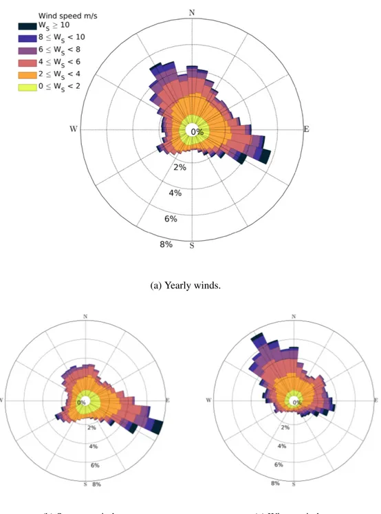
Seasonal and yearly wind rose plots made for the BSI using the HRDPS model solutions are shown in Figure 6. The yearly average wind speed is 4.01 ± 2.46 m s−1 but this value is
higher (4.52 ± 2.48 m s−1) and lower (3.62 ± 2.34 m s−1) in winter and summer, respectively. Winds below the yearly average are more common (64%) in the summer relative to winter (48%). The strongest modelled winds blow at 19.57 m s−1. In the range 105◦to 125◦, wind speeds greater than 10 m s−1 happen 0.42 ± 0.10% of time, making them 5±4 times more
frequent in this direction than they are on average everywhere else (0.09 ± 0.02%).
Winds mainly blow from the three general directions NNW, ESE, and SW, whose rel-ative importance changes throughout the year. In winter, winds blowing from the NNW (300−360◦) are dominant accounting for 38% of data. Winds from a similar range (300−30◦) are still notably present in summer but then account 29%. Easterly winds appear in the distri-butions of both seasons in the range 90 − 130◦. For this range, they account for 15% of data in the winter and are twice as frequent (28%) in the summer. Winds from the SW (200 − 240◦)
26
(a) Yearly winds.
(b) Summer winds. (c) Winter winds.
Figure 6: Wind provenance from the HRDPS wind model. Panel a) shows data from Febuary 2017 to Febuary 2018. Panel b) shows data from April 2017 to November 2017. Panel c) shows data from November 2017 to April 2018.
27
1.4.3 Temporal variability
1.4.3.1 Seasonal scale
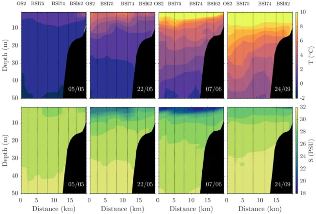
Synoptic representation of temperature and salinity in the first 50 m of depth are shown in Figure 7 for transect T3 (see Figure 2) running from the offshore stations to the inside of the bay. Positions along T3 are given in the following as distance in kilometers from the station furthest offshore. Profiles are gathered over two consecutive days for each sampling campaign. Over the entire 2017 data set, density and salinity are highly correlated (R= 0.99) whereas for density and temperature R = 0.82. Salinity data is therefore reliably indicative of density. The maximum buoyancy frequency over all depths Nmax2 is used in what follows as a measure of stratification. N2
maxvalues related to the transects shown in Figure 7 compose
Table 4.
Minimum average stratification (N2
max= 1.6±0.79×10
−3s−2) is measured in early May.
At this time, stratification (Nmax2 = 3.3 × 10⁻³s−2) is 2.4 times stronger inside the bay (20 km) than on average elsewhere on the transect (N2
max = 1.4 ± 0.41 × 10
−3s−2). Averaged over the
surface five meters, water at the 20 km station is 1.7◦C warmer and 0.4 PSU less salty than the other stations averaged together.
By the end of May, average stratification increases by an order of magnitude (N2 max =
2.0 ± 2.6 × 10⁻²s−2). Stratification is then maximum, comprising the two largest N2
maxvalues
measured over all (N2
max= 7.8 × 10⁻²s−2and Nmax2 = 3.7 × 10⁻²s−2) interspersed with values
often an order of magnitude smaller, see Table 4. Opposite to early May, stratification is now stronger outside the bay (0 − 15 km) where on average N2
max = 2.9 ± 3.0 × 10⁻²s−2 relative
to inside the bay (15 − 20 km) where N2
max = 4.7 ± 2.1 × 10⁻³ s−2. The horizontal salinity
difference is stronger with water between 15 and 20 km saltier than water in the 0 − 15 km range by 4.8 PSU. The temperature difference for the same regions is comparable to early May in magnitude (1.6◦C ) but opposite in direction.
28 (dd/mm) / (km) 0.00 2.29 4.71 7.86 11.50 15.00 17.12 20.22 05/05 1.8 1.9 1.1 1.4 1.3 0.69 1.5 3.3 22/05 78 8 11 11 37 3 4.1 7 07/06 23 30 17 25 25 22 30 25 24/09 6.5 5.8 3.9 2.8 5 4.9 14 31 Table 4: N2
max (10−3s−2) for the profiles along T3 at different times of the season. Columns
indicate distance from the station furthest offshore.
The strongest stratification averaged across all stations is reached in early June with N2
max= 2.5±0.4×10⁻²s−2. Stratification is also more horizontally homogenous as is reflected
by the decreased standard deviation. The largest surface temperature and salinity gradients are now further inside the bay between 17 and 20 km. The water at 20 km is colder and saltier than the rest of the stations averaged together by 3.0◦C and 3.5 PSU.
The September measurements resemble those in early May. Stratification at 20 km is 5 times stronger (Nmax2 = 3.1 × 10⁻² s−2) than the rest of the stations averaged (Nmax2 = 6.2 ± 3.7 × 10⁻³ s−2). Average stratification decreases to N2
max = 9.3 ± 9.4 × 10⁻³ s−2. As
in early May, the least dense water is found near 20 km, where water is 1.9 PSU less salty than the rest of the stations averaged. No horizontal gradient of temperature appears in these measurements.
During summer, the GSL is a three layer stratified system (Galbraith, 2006). Charac-teristic temperature and salinity values are 1◦C to 7◦C and S > 32.5 PSU for the gulf bottom
water (GBW), and the cold intermediate layer (CIL) is defined by summer temperatures be-low 1◦C. According to these definitions, 42% and 3% of measurements match the properties
characteristic to the CIL and GBW respectively. Seasonal evolution of the CIL’s vertical structure has been detailed by Cyr et al. (2011). They show that during spring, when most of our measurements were collected the CIL’s core is centered around 60 m and 50-100 m thick. The average depth of our measurements is 60 ± 30 m in the CIL, and 133 ± 15 m in the GBW. Influence of the CIL was therefore seen in BSI at depths typical of other areas in the
29
GSL during spring, while GBW was only measured deep in the channels or at the offshore stations.
Figure 7: Seasonal change in temperature (top) and salinity (bottom) along transect T3. Dis-tance along T3 with 0 at the offshore station is on the x axis. Date of sampling is written in the bottom right corner of each panel.
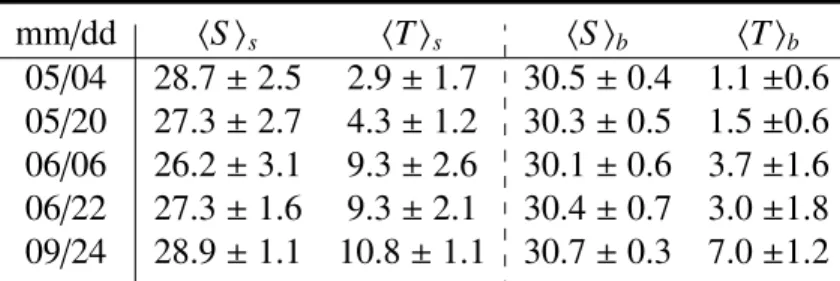
Table 5 lists average temperature and salinity for the top 10 meters and the 10 to 30 m layer, along with standard deviations. Salinity in both layers decreases from May to early June, then increases back to its May values by the end of September. Maximum to minimum difference is 4.9 times larger (2.7) in the surface compared to the 10 to 30 m layer (0.6). Salinity is most variable in early June for both layers but 5 times more so near the surface (SD = 3.2 PSU) than underneath (SD = 0.6 PSU). Near the surface, change in salinity is fast (∼ 0.5 PSU/week) from May to June, then slower (∼ 0.1 PSU/week). Underneath, the tendency is the same but rates are an order of magnitude smaller.
30 mm/dd hS is hT is hS ib hT ib 05/04 28.7 ± 2.5 2.9 ± 1.7 30.5 ± 0.4 1.1 ±0.6 05/20 27.3 ± 2.7 4.3 ± 1.2 30.3 ± 0.5 1.5 ±0.6 06/06 26.2 ± 3.1 9.3 ± 2.6 30.1 ± 0.6 3.7 ±1.6 06/22 27.3 ± 1.6 9.3 ± 2.1 30.4 ± 0.7 3.0 ±1.8 09/24 28.9 ± 1.1 10.8 ± 1.1 30.7 ± 0.3 7.0 ±1.2
Table 5: Average temperature and practical salinity shown with standard deviation for the top 10 m hS , T is, and for the 10 to 30-m layer hS , T ib.
Average temperature increases throughout the season in the top 30 m with the exception of a small drop (top 10 m: 0.4◦C , 10-20 m: 0.5◦C ) in late June. Near the surface, temperature
rises at a rate of 0.6◦C /week, and 2.1◦C /week in early and late May respectively. Change is then much slower (0.1◦C/week) until September. Temperatures are most variable (SD =
2.6◦C ) in early June near the surface but maximum standard deviation (SD= 1.8◦C ) is found two weeks later in the 10 to 30 m layer.
The composition of the BSI water and evolution of its surface water is summarized by the TS diagram shown on Figure 8. No salinity appears greater than ∼ 33 PSU and the bulk of the data is found at values associated with the CIL. The surface water becomes warmer and more brackish at an increasing pace from May to early June. It then continues warming and becomes saltier until September. Salinity then ressembles early May conditions with temperatures 7.96◦C , and 1.06◦C warmer respectively in the top 10 m, and 10 to 30 m layer.
31
Figure 8: Temperature and salinity data and it’s seasonal variability. Marker shape indicates sampling campaign and depth is shown by the color axis. ’*’ symbols in the legend mark sampling campaigns where only a subset of stations are visited. Salinities as low as 16.52 where measured but only in the 06/06 campaign and are not shown for clarity. Boxes are centered on the surface 10 meter mean values (see Table 5) for each campaign and are 2 standard deviations wide in both directions.
Evolution of σH, the density profile averaged horizontally across all stations is shown
in Figure 9 for the top 30 m. The maximum standard deviation of σH, reflecting spatial
difference between averaged profiles, is 2.17 kg m−3at measured z= 4 m, and values decrease with depth. In the top 5 meters, σH variations around the seasonal mean can reach 25%.
32
Figure 9: Evolution of the average water column density structure through the season. The color axis shows density, whereas the overlaid solid black lines show temperature. Standard deviation between stations is computed for every campaign and shown on the left. Dashed lines indicate times of sampling campaigns.
Discharge time series of local, regional, and large scale fresh water sources are shown on Figure 10. The yearly mean discharge of the Rapides river is 16.6 m3 s−1 making it the largest contributor (74.4%) to the yearly averaged value for all of BSI’s tributaries (22.3 m3s−1)
presented by Proc´ean (1999). During peak discharge (April to July) the climatology averages to more than double the yearly value (36.4 m3s−1) with the maximum (78.5 m3s−1) happening
on May 24. As sampling was conducted two weeks apart around the spring freshet, maxi-mum local discharge therefore happened 14±14 days before minimaxi-mum density was measured in the BSI. The maximum monthly and daily discharges of the St. Lawrence and Moisie Rivers happen respectively 22±14 and 23±14 days prior to the early June measurements (2017/06/07), when minimum salinity was observed in the BSI (SH = 19.8 PSU, z < 2).
Daily averaged salinity data from a DFO buoy near Rimouski, upstream of the BSI shows a seasonal minimum of S = 15.7 on May 24.
33
Figure 10: Time series of river discharge for three rivers, Rapide (local), Moisie (regional), and St. Lawrence (large scale). The area between climatological maximums and minimums is shown in grey. For the middle and bottom panels the solid black line shows 2017 values. Since these values are unavailable for rivi`ere des Rapides, the climatology mean is shown. Dashed lines indicate times of sampling campaigns. Top two panels made from CEHQ tide gauge data, and bottom panel shows RIVSUM.
1.4.3.2 Tidal scale
CTD data from the June 2017, September 2017, and May 2018 campaigns is used to reconstruct temperature and salinity fields on T1 at several moments of the tidal phase, as shown on Figure 11. Tidal range during these three measurements was respectively r = 1.52 m, r = 1.42 m, and r = 2.34 m. We define ∆T, ∆S positive along xc, as the temperature
and salinity difference between reconstructed profiles averaged over the 5 surface meters at a given time. Its indices define the concerned stations; south (xc ∼ 1 km), center (xc ∼ 2.5
34
and south, ∆TNC is the difference between temperatures north and center, and ∆TCS is the
difference between temperatures center and south. Values of ∆T and ∆S are presented in Table 6 for the three reconstructed tide cycles at tide phases matching the panels of Figure 11. Tidal evolution of the horizontal stratification across T1 seems variable. In June,∆TNS
and ∆SNS were of opposing signs and both switched direction during the tidal cycle. In
September and May, ∆TNS and ∆SNS remained in the same direction throughout the tidal
cycle, but reached minimums at ebb and low tide respectively. Note however that∆SS N is of
opposite sign during these two measurements.
HT+t ∆TNS (◦C) ∆SNS (PSU) ∆TCS (◦C) ∆SCS (PSU) ∆TNC (◦C) ∆SNC (PSU)
0 -0.44 0.85 -0.24 0.73 -0.20 0.12 3 -0.19 0.81 -0.09 0.40 -0.10 0.41 6 1.31 -0.48 1.07 -0.45 0.24 -0.04 9 0.49 -0.04 0.97 -0.37 -0.47 0.32 0 -0.48 -0.29 -0.47 0.03 -0.01 -0.33 3 -0.37 -0.02 -0.38 0.32 0.00 -0.33 6 -0.37 -0.69 0.05 -0.16 -0.42 -0.52 9 -0.72 -0.61 -0.52 -0.34 -0.21 -0.27 0 -0.81 1.89 -0.47 1.52 -0.34 0.37 3 -0.37 0.61 0.14 0.28 -0.51 0.32 6 -0.22 0.09 0.09 -0.16 -0.32 0.24 9 -0.82 1.38 -0.46 1.09 -0.36 0.29
Table 6: Temperature and salinity difference between the south, center and north sampling stations for the reconstructed tide cycles of June 2017 (top row), September 2017 (middle row), and May 2018 (bottom row). The left column indicates tidal phase in hours after high tide.
The largest∆TS N and ∆SS N values were measured in June at low tide, and in May at
high tide. Both of these maxima have in common that most of the variation happens between the south and center stations. ∆SCS and∆SNC have been observed in opposition, placing the
saltiest water in the center of T1 as in September (HT+3), or to the sides as in June (HT+9) and in May (HT+6). This has also been seen in ∆TCS and∆TNC notably in June (HT+9) and
35
Figure 11: Reconstructed temperature (color) and salinity (solid lines) fields along T1. Columns are June 2017 (left), September 2017 (center), and May 2018 (right) repeated tran-sects. Rows are approximately corresponding tidal phase, as is written in hours after high tide. Note the different color axes for each column.