Science Arts & Métiers (SAM)
is an open access repository that collects the work of Arts et Métiers Institute of Technology researchers and makes it freely available over the web where possible.
This is an author-deposited version published in: https://sam.ensam.eu Handle ID: .http://hdl.handle.net/10985/17461
To cite this version :
Solenne MONDESERT-DEVERAUX, Rachele ALLENA, Denis AUBRY - In silico approach to quantify nucleus selfdeformation on micropillared substrates - Biomechanics and modeling in mechanobiology - Vol. 18, n°5, p.1281–1295 - 2019
Any correspondence concerning this service should be sent to the repository Administrator : [email protected]
https://doi.org/10.1007/s10237-019-01144-2
In silico approach to quantify nucleus self‑deformation
on micropillared substrates
Solenne Mondésert‑Deveraux1 · Denis Aubry1 · Rachele Allena2
Abstract
Considering the major role of confined cell migration in biological processes and diseases, such as embryogenesis or meta-static cancer, it has become increasingly important to design relevant experimental set-ups for in vitro studies. Microfluidic devices have recently presented great opportunities in their respect since they offer the possibility to study all the steps from a suspended to a spread, and eventually crawling cell or a cell with highly deformed nucleus. Here, we focus on the nucleus self-deformation over a micropillared substrate. Actin networks have been observed at two locations in this set-up: above the nucleus, forming the perinuclear actin cap (PAC), and below the nucleus, surrounding the pillars. We can then wonder which of these contractile networks is responsible for nuclear deformation. The cytoplasm and the nucleus are represented through the superposition of a viscous and a hyperelastic material and follow a series of processes. First, the suspended cell settles on the pillars due to gravity. Second, an adhesive spreading force comes into play, and then, active deformations contract one or both actin domains and consequently the nucleus. Our model is first tested on a flat substrate to validate its global behaviour before being confronted to a micropillared substrate. Overall, the nucleus appears to be mostly pulled towards the pillars, while the mechanical action of the PAC is weak. Eventually, we test the influence of gravity and prove that the gravitational force does not play a role in the final deformation of the nucleus.
Keywords Mechanical forces · Nucleus self-deformation · Micropillared substrate · In silico model
1 Introduction
To survive, cells need to constantly adapt to their environ-ment by altering their morphology and physiology (Benja-min and Hillen 2003; Mammoto and Ingber 2010; Versaevel et al. 2012; Swift et al. 2013). During confined migration, for instance, cells undergo important strains in order to be able to squeeze enough and migrate through sub-cellular and sub-nuclear pores as far as the nucleus, the stiffest cellular
organelle, enables it (Friedl et al. 2011; Wolf et al. 2013). Impressively, cancerous cells are even able to break the nuclear lamina to soften the nucleus and to invade healthy tissues across tiny pores (Denais et al. 2016; Bell and Lam-merding 2016). As such, the evolution of nuclear morphol-ogy can be used as a biomarker in the diagnosis and prog-nosis of cancer patients (Schirmer and de las Heras 2014; Ermis et al. 2016).
In order to characterize such cells and analyse their behaviour in confined environments, patterned microflu-idic devices are often used (Lu et al. 2004; Rosenbluth et al. 2008; Davidson et al. 2009). Micropillars are most commonly employed as an array of thin beams in traction force microscopy to access the interaction forces between a cell and its substrate (Tan et al. 2003; du Roure et al. 2005; Ghibaudo et al. 2011). Additionally, by controlling the mate-rial used, the size of the pillars and the gap size between pil-lars, they can serve to control the shape of the nucleus (Pan et al. 2012; Hanson et al. 2015) and investigate the process of nuclear self-deformation induced by mechanical forces generated by the topological surface (Davidson et al. 2010;
* Rachele Allena
1 Laboratoire MSSMat UMR CNRS 8579, CentraleSupélec,
Université Paris-Saclay, 8-10 Rue Joliot Curie, Gif-Sur-Yvette, Paris, France
2 LBM/Institut de Biomécanique Humaine Georges Charpak,
Arts et Metiers ParisTech, 151 Boulevard de l’Hôpital, Paris, France
Badique et al. 2013; Liu et al. 2017, 2018). These recent experiments offer a new insight on nuclear deformation and raise further questions: is gravity driving this movement (Pan et al. 2012)? Is the nucleus being pulled or pushed (Davidson et al. 2010; Badique et al. 2013; Hanson et al. 2015)? Indeed, intense contractile actin fibres have been observed at two locations in the cell: above the nucleus and around the pillars beneath the nucleus (Hanson et al. 2015; Davidson et al. 2015; Fig. 1a). The fibres above the nucleus form a dome-like actin cap called the perinuclear actin cap (PAC) (Khatau et al. 2009). This PAC domain has three fixa-tion points in the cell: it is anchored at its both ends to a spe-cific type of focal adhesions (FAs) and, in its middle, to the nuclear lamina via linker of nucleoskeleton and cytoskeleton (LINC) complex (Maninova et al. 2017; Fig. 1b). The PAC thus forms a direct mechanosensing link from the extracel-lular matrix to the nucleus (Kim et al. 2012) and has been found to be a regulator of cell migration (Kim et al. 2014).
When using microfluidic devices, one may observe suc-cessive steps. From a suspended state, the cell gently comes in contact with the pillars, adheres and then spreads, polar-izes and eventually crawls over the substrate.
Spreading can be divided into two main phases. The first phase is a completely passive one during which the cell set-tles on the substrate under the action of gravity only and
deforms depending on its own overall stiffness. The second phase is an active one during which the cell protrudes and contracts through polymerization and depolymerization.
Once the cell has touched the underneath substrate, it starts developing the FAs to create a mechanical link between the intra-cellular actin filaments and the substrate surface (Aber-crombie et al. 1970). Then, FAs play the role of anchoring points that restrain cell contraction while promoting cell protrusion at the leading edge and nucleus self-deformation through the pillars (Morgan et al. 2007; Geiger et al. 2009; Liu et al. 2017, 2018). It has been observed that the nucleus may undergo large and severe deformations as a function of the cellular phenotype and the nuclear size. Additionally, external forces may highly modify the nucleus shape as well as the chromatin organization inside it and consequently its gene expression. According to these experimental observations, it is essential to decipher the mechanical processes triggering the nucleus large strains which may be responsible for impor-tant cellular functions such as migration or proliferation.
Our main objective is to analyse the nuclear behaviour as a function of the micropillared substrate geometry (i.e. pillars height, width and interspace) and the contractile fibre network formed by the cell around the nucleus itself. This particular aspect has been so far poorly observed and inves-tigated from an experimental point of view and never been
(a)
(b)
Fig. 1 a Sketch of the cell and nucleus morphologies once it has penetrated between the micropillars. The actin fibres constitut-ing the PAC and the bottom zone are represented in blue and green, respectively. The former are tangentially oriented, whereas the latter are radially oriented. b Geometrical representation of the cell com-ponents as well as the PAC (ΩPAC) and the bottom zone (Ωbottom) in
our numerical model at t =0. rc and rn are the cell and nucleus radii,
respectively, rcp and ecp the external radius and the thickness of the
cytoplasm, and em the membrane thickness. cc , pb and pt are the cell
centre and a bottom and a top points, respectively, used for post-processing
numerically modelled. Therefore, we believe that our com-putational approach can bring new insights in understanding how the nucleus responds to its environment and what are the mechanical forces driving such behaviour.
1.1 Modelling of cell–substrate interaction
Most of the models that can be found in the literature focus on the interactions between the cell and a flat substrate and can be divided into three main categories: analytical, dis-crete and continuum models.
Analytical models do not require extensive computational implementation, but they only provide global information of spreading dynamics in various conditions. The very first models aimed at investigating the evolution (i.e. progression in size and morphology) of the contact surface (Cuvelier et al. 2007) or the influence of ligand density gradient on cell kinematics (Sarvestani and Jabbari 2008). More recently, some models have also taken into account the active forces triggered by the acto-myosin network (Nisenholz et al. 2014) or the mechanotransduction feedback from the nucleus to the FAs (Cao et al. 2015).
Discrete models allow to analyse the intra-cellular rear-rangement since they physically represent the cytoskeleton as a network of connected bars (i.e. tensegrity models) (Ingber 2003). Tensegrity has been coupled to divided-media theory (or cytoskeleton divided medium method) to assess mecha-notransduction during spreading with just one type of ten-sile filaments (Milan et al. 2013) or with the actin filaments, intermediate filaments and microtubules (Fang and Lai 2016).
In continuum models, whether they are two (2D) or three (3D) dimensional, the cell is considered as a continuum solid or fluid domain and no organelle is physically represented, but the nucleus. Such models are able to provide informa-tion at both the global and the local levels. Some studies focus on the first step of the spreading mechanism, model-ling receptor–ligand binding, which can only lead to a lim-ited deformation of the cell (Liu et al. 2007; Golestaneh and Nadler 2016), although the use of membrane reservoirs can influence its extent (Étienne and Duperray 2011). Another method consists in modelling spreading mechanism through a unique force accounting for both ligand–receptor binding and active acto-myosin cytoskeleton tension forces, and it can be used to study more specifically the dynamics of the nucleus during cell spreading (Zeng and Li 2011a, 2012). One model proposed a two-step process: (1) a purely passive spreading and (2) an active actin action to help the cell to spread further (Fan and Li 2015a, b). As for modelling the interactions between the cell and a micropatterned substrate, a first attempt was made by Hanson et al. (2015) to investi-gate whether the nucleus is being pulled or pushed in pillars groves. Nonetheless, the question is still open and mainly motivates our present study.
In line with our previous works (Allena and Aubry 2012; Deveraux et al. 2017), we propose a continuum finite ele-ments model to simulate cell behaviour over the flat and micropatterned substrates coated with adhesive fibronectin. As mentioned above, our main objective is to depict the nucleus self-deformation as a function of the micropillared substrate geometry and the actin network around the nucleus itself. This will allow us to computationally determine whether the nucleus is able or not to penetrate between the pillars and what mechanical forces drive such penetration.
The 2D cell approximation in our model is constituted of the nucleus, the cytoplasm and the membrane and is described as a visco-hyperelastic material under large deformations. During the process, the cell is submitted to (1) gravity, (2) a spreading and adhesion force, (3) a contact force with the substrate surface and (4) an active contrac-tile strain. The active contraccontrac-tile strain allows us to explore whether the actin filaments on the top and at the bottom of the nucleus push or pull it down, respectively.
2 The model
2.1 Cell geometry and constitutive laws
Let us consider the initial cellular 2D domain Ωc constituted by the nucleus Ωn and the cytoplasm Ωcp , which includes the membrane Ωm (Fig. 1b). Because of the symmetry condi-tions, the nucleus is a semicircle of radius rn , whereas the cytoplasm and the membrane are two semi-annuli. The cyto-plasm has an internal radius rn , an external radius rcp and a thickness ecp . The membrane has an internal radius rcp , an external radius rc and a thickness em . Each component of the cell is defined by a spatial characteristic function gi which is the composition of a regularized Heaviside function H and a level set function li (where the subscript i indicates the component). The former is a classical step function which value is 0 for negative argument and 1 for positive argument. Then, in our model, the function gi is positive inside the cor-responding domain and negative outside and reads
(1) gc= H◦lc= H◦(p− c2 c,p− r 2 c ) (2) gn= H◦ln= H◦ ( p− c2c,p− r2n ) (3) gcp= H◦lcp− gn= H◦ ( p− c2 c,p− r 2 cp ) − gn (4) gcp= gc− gn (5) gm= gc− gcp− gn
with p being the initial configuration (t = 0, t being the time) of any point in the system and cc,p the centre of the cell of coordinates (cx, cy
) .
In the cell, both the cytoplasm and the nucleus are consti-tuted by a solid and a fluid phase, as proposed in Fig. 2. The nucleus is composed by the lamina (solid) and the nucleo-plasm (fluid), and the cytonucleo-plasm by the cytoskeleton and the membrane (solid) and the cytosol (fluid).
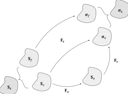
As in a Kelvin–Voigt model, the overall stress Sc and deformation Fc of the cell are given by
where the subscripts s and f indicate solid and fluid, respectively.
2.1.1 The solid phase
The second Piola–Kirchhoff stress Ss in the solid phase can be expressed as
where Fa is the active deformation tensor which will be detailed later in Sect. 2.2.5, Se is the second Piola–Kirchhoff stress for the elastic part of the solid phase and Ja is its deter-minant. In fact, as proposed in the previous works (Rodri-guez et al. 1994; Lubarda 2004; Muñoz et al. 2007; Cheru-bini et al. 2008; Allena et al. 2010; Ambrosi et al. 2011; Nobile et al. 2012; Allena and Aubry 2012; Golestaneh and (6) Sc= Ss+ Sf (7) Fc= Fs= Ff (8) Ss= JaF−1a SeF−Ta
Nadler 2016; Deveraux et al. 2017), we model the cell con-tractility as an active strain through the decomposition of the deformation gradient Fc (see Fig. 2) which then reads with Fe being the elastic deformation gradient tensor. As shown in Ambrosi and Pezzuto (2011), the active strain approach is mathematically more robust than the active stress one and if the active strain can be reinterpreted in terms of active stress, no new free parameters need to be tuned. Additionally, some interesting works with promising results have been proposed to investigate the physiological effectiveness of the obtained model (Stålhand et al. 2008; Murtada et al. 2010).
Among the different isotropic material models available to describe the cell as a hyperelastic solid continuum, one may distinguish between (1) standard Saint–Venant material (Allena and Aubry 2012; Fan and Li 2015b) whose elas-tic energy depends on the first invariant I1= Tr
(
Ce) and I2,SV= Tr(C2e) , with Tr being the trace of a tensor and the
Ce= F
T
eFe the symmetric right Cauchy–Green tensor, (2) the neo-Hookean material (Jean et al. 2003; Mokbel et al. 2017) which depends on I1 and on the third invariant I3= det
(
Ce) ,
with det being the determinant of a tensor, (3) the poly-convex Mooney–Rivlin material (Zeng and Li 2011b; Wang et al. 2017) which depends on I1 , I3 and I2= det
(
Ce )
Tr(C−1e )
(Holzapfel 2000) and (4) the Yeoh model which nonlinearly depends on I1 , I2 and I3 (Yeoh 1993).
In the cell, the cytoskeleton and the lamina are com-posed by different types of biopolymers (i.e. actin fibres, intermediate filaments, microtubules, etc.), which may (9)
Fc= FeFa
Fig. 2 Different phases of the constitutive model used to describe the mechanical behaviour of the cytoplasm and the nucleus
undergo a significant strain stiffening when deformed. It is the case for actin fibres and strains less than 10%, as reported in Storm et al. (2005) and Erk et al. (2010), but no experimental data are available for strains higher than 10%. According to the graphics presented in these works, one may deduce that the stiffness of the actin fibres increases exponentially as the strain increases too. Such a behav-iour is unlikely to be mechanically realistic and would completely inhibit the whole cell deformation. However, it is possible that actin fibres undergo sequential deforma-tion (i.e. stiffening) and unfolding (i.e. relaxadeforma-tion), which results in a saw-tooth pattern of the stiffness as presented in Bao and Suresh (2003). Given such observations and since in our model large strains occur (especially for the cytoskeleton), we have decided to employ a visco-hyper-elastic Yeoh material model whose parameters have been reasonably tuned in order to take into account the stiffening for small deformations.
The material energy WY can be written as
with 𝛼1, 𝛼2, 𝛼3 and 𝛽 being the scalars and Γ a convex func-tion of Je= det ( Fe ) = det(Ce )1∕2 . More specifically, we consider Γ = 𝜆Y 2ln ( Je)2− 3𝛼1J 2∕ 3 e − 3𝛽J 4∕ 3 e as defined in Fried and Johnson (1988), and according to Bonet et al. (2015), we can write while 𝛼2= − 𝛾𝛼1 = − 𝛾 [E c(1+𝜈c) 2 ] and 𝛼3= 𝛾𝛼1= 𝛾 [E c(1+𝜈c) 2 ] , with 𝛾 being a scalar, Ec= Engn+ Ecpgcp , 𝜈c the cell Pois-son’s ratio, 𝛽 = 0.2𝜇e
2 , 𝜇e and 𝜆e the cell Lamé’s coefficients. The second Piola–Kirchhoff tensor Se is derived from WY as follows:
Through some algebraic manipulations, Eq. (13) becomes (10) WY = 𝛼1 ( I1− 3I 1 3 3 ) + 𝛼2 ( I1− 3I 1 3 3 )2 + 𝛼3 ( I1− 3I 1 3 3 )3 + 𝛽 ( I2− 3I 1 3 3 ) + Γ(Je) (11) 𝛼1+ 𝛽 = 𝜇e 2 (12) 𝜆Y= 𝜆e+ 2 3𝜇e (13) Se= 2 𝜕WY 𝜕Ce (14) S e= 2 [ 𝛼1+ 2𝛼2 ( I1− 3I 1 3 3 ) + 3𝛼3 ( I1− 3I 1 3 3 )2]( I− I 1 3 3C −1 e ) + 2𝛽 ( TrCeI− Ce− 2I 2 3 3C −1 e ) + Γ�C−1 e
2.1.2 The fluid phase
Here, we consider a classical Newtonian viscous fluid which must be described in the Lagrangian configuration to ensure the compatibility with the solid phase.
The Cauchy stress tensor 𝝈f is expressed as
where 𝜆f and 𝜇f are the isotropic and deviatoric viscosi-ties, respectively. Df is the Eulerian cell rate of deformation gradient which is expressed with respect to the Lagrangian coordinates as
with the superscript T indicating the transpose of a matrix. Since 𝐅f= 𝐅c and 𝐂f= 𝐂c , the Cauchy–Green tensors of the fluid phase and of the global cell, respectively, and by sub-stituting the expression of 𝝈f and Df , we obtain
Finally, given dC−1 c dt = − C −1 c dCc dt C −1 c , Eq. (17) becomes
2.2 The cell and its environment
The cell reacts and interacts with its environment which is constituted of an underneath flat or micropillared substrate. In the following, we detail the different forces to which the cell is submitted and that affect its global behaviour.
2.2.1 The underneath substrate
The substrate may be flat or structured. In both cases, it is defined by a spatial characteristic function gi (where the subscript i indicates the substrate type) which, as defined in Sect. 2.1, is a composition of a smooth Heaviside function H and level set function li which reads
(15) 𝝈 f = 𝜆fTr ( Df)I+ 2𝜇fDf (16) Df= 𝐅−Tf d𝐂f dt 𝐅 −1 f (17) 𝐒f= Jc𝐅−1 c 𝛔c𝐅−Tc = Jc𝜆f 2 Tr ( 𝐅−T c d𝐂c dt 𝐅 −1 c ) C−1c + Jc𝜇fC−1c d𝐂c dt C −1 c (18) 𝐒f= Jc𝜆f 2 Tr ( C−1c d𝐂c dt ) C−1c − Jc𝜇f dC−1c dt (19) gflat= H◦lflat= H◦ ( −y + yflat ) gmp= H◦lmp= (20) H◦ {[| || ||x− xmp− ( smp+ wmp ) round ( x− x mp smp+ wmp )| || || 4 + |||y − ymp||| kmp − (w mp 2 )4] + gflat }
where the subscripts flat and mp indicate ‘flat’ and ‘micropil-lared’, respectively, and x and y are the coordinates of any particle in the system. The flat substrate gflat is represented by a semi-infinite place at yflat position with respect to the
y-axis. The micropillared substrate is represented by a series
of pillars of width wmp , space of smp and height obtained through the coefficient kmp . We can consider an infinite num-ber of pillars as a function of the first one which is posi-tioned in xmp and ymp . Finally, round is a function that rounds to the nearest integer.
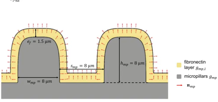
For both gflat and gmp , we consider a thin layer cov-ered with fibronectin and where the cell can therefore adhere. The layer is called gflat,l and gmp,l for the flat and micropillared substrate, respectively, (Fig. 3). In the case of the flat substrate, the layer is obtained by subtracting
gflat from a higher flat substrate (i.e. higher y coordinate, yflat,l>yflat ). In the case of the micropillared substrate, gmp
is subtracted from a wider (i.e.wmp,l>wmp ), higher (i.e.
hmp,l>hmp thus kmp,l>kmp ) and with smaller inter-pillar
space (i.e. smp,l<smp ) micropillared substrate (Fig. 3). In both cases, the thickness of the fibronectin layer ef has been set to 1.5 µm. Such a value has been chosen assuming that although in reality the fibronectin thickness is in the order of some nanometres, the cell must ‘sense’ this adhering mole-cule at the microscale. From a numerical point of view, such a thickness, which is in the order of the mesh size, allows to precisely detect the adhesion between the cell and the fibronectin through the adhesion force fas (see Sect. 2.2.4).
The outward normal vectors nf and nmp (Fig. 3) to the flat and micropillared substrate, respectively, are given by
(21)
nf= ∇xlflat ∇xlflat
2.2.2 The gravity force
At first, the cell is suspended and settles over the substrate due to the gravity fg . Nevertheless, for numerical and con-vergence purposes, such a force cannot be applied all of a sudden but rather smoothly over a period of time Tg . Then, it reads
with 𝜌p being the initial cell density, g the gravitational acceleration, and iy the vertical unit vector. tg is a temporal characteristic function which reads
with t being the time and Tg0 the upper limit of Tg (Fig. 4). Once the cell touches the substrate, the gravity is main-tained, and two further forces start to act: the contact force
fct and the adhesive spreading force fas.
2.2.3 The contact force between the cell and the substrate
The contact force fct automatically applies once the cell approaches the substrate, whether it is flat or micropillared, over a very thin layer corresponding to the superposition between the cell and the substrate. Then, it is approximated by a volume force as proposed in our previous work (Deveraux et al. 2017). (22) nmp= ∇xlmp ∇xlmp (23) fg = − 𝜌ptggiy (24) tg= H◦lg= H◦(− t + Tg0 )
Fig. 3 Pillars ( gmp ) in grey with the superposed layer of fibronectin ( gmp,l ) in yellow. The red arrows represent the outward normal vector nmp .
We employ here a penalization technique via the level set functions gflat and gmp which allow to measure the distance and the interpenetration between the cell and the substrates.
Then, fct reads
where 𝜇ct is the penalization coefficient and the cofactor matrix is defined as cof(Fc
)
= JcF−Tc . Since we employ here a Lagrangian description, the normal vectors nflat and
nmp must be brought back to their initial configuration by multiplying them by cof(Fc
) .
2.2.4 The adhesive force
The volume adhesive spreading force fas allows to mimic the FAs maturation via the recruitment of scaffolding and sig-nalling components (Geiger et al. 2009). When the cell gets closer to the substrate, the adhesive spreading force comes into action on the portions of the substrate coated with ECM proteins such as fibronectin. As in other works (Zeng and Li 2011a; Fan and Li 2015b; Fang and Lai 2016), we do not get into the molecular details of spreading, but design a sin-gle body force accounting for both the actin polymerization
(25)
fct= {
𝜇ctgflatcof(Fc )
nflat, on flat substrate
𝜇ctgmpcof (
Fc )
nmp, on micropillared substrate
at the cell membrane (Keren 2011) and the formation of adhesion complexes between the cell and its environment (Fig. 5). This nonlinear force, attracting the cell towards the substrate, is one of the novelties of this model. Inspired by the work of Sauer (2016), we consider an overlayer of fibronectin surrounding the substrate, in which the spread-ing force will act on the cell’s membrane. Our model only considers the case of a homogeneous fibronectin distribution over the substrate and thus a continuous overlayer.
fas is radial and is applied over a period Tas , starts at
t= Tg0 , reaches its maximum value at t = Tas0 and is main-tained afterwards (Fig. 4). The force is a body force, but it is applied at the thin intersection between the cell membrane and the fibronectin layer (Sect. 2.2.1). It reads
where cof(Fc )
nc,p is the outward normal to the cell in the reference configuration. Such a normal is computed at the cell boundary, but it is easily extended inside the cell mem-brane through the gradient of memmem-brane level set function
lm . tas is a temporal characteristic function defined as
(26) fas= { 𝜇as(x, t)gf,lgmtascof ( Fc)nc,p, on flat substrate 𝜇as(x, t)gmp,lgmtascof ( Fc ) nc,p, on micropillared substrate (27) tas= H◦las= H◦ [( t+ Tg0)(− t + Tas0)]
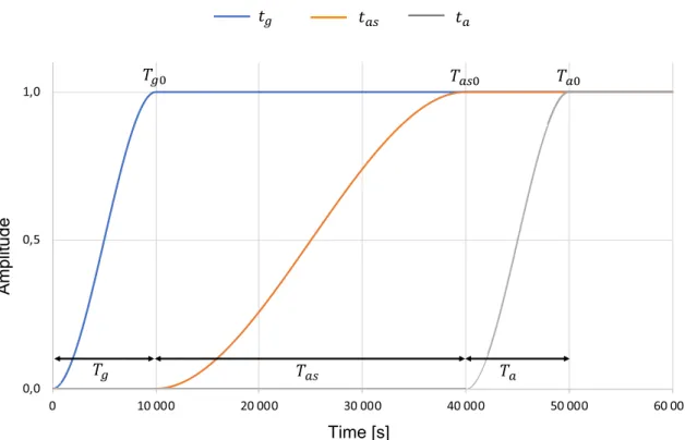
Fig. 4 Representation of the temporal characteristic functions neces-sary to describe the evolution of the gravity fg [i.e. the function tg in
blue, Eq. (24)], the adhesive spreading force fas [i.e. the function tas
in orange, Eq. (27)] and the active strains Fa,PAC and Fa,bottom [i.e. the
function ta in grey, Eq. (35)]. Each function starts from 0 and reaches
the maximum value 1 after a specific period of time: Tg= 10,000 s
for the gravity, Tas= 30,000 s for the adhesion spreading force and Ta= 10,000 s for the active strains. The maximum value 1 is achieved
with Tas0 being the upper limit of tas (Fig. 4).
𝜇as(x, t) is the spreading coefficient which satisfies the following partial differential equation
where 𝜇as0 and 𝜇as,max are the two positive scalars. Through this partial differential equation, 𝜇as(x, t) starts to smoothly increase as soon as the cell touches the substrate until it reaches a maximum value 𝜇as,max . Equation (28) allows to mimic the FAs maturation via the recruitment of scaffolding and signalling components (Geiger et al. 2009).
2.2.5 The active strains
Once the cell has settled on the substrate due to the gravity fg , spread and adhered on the micropillars due to fas , it starts to actively deform. In fact, during spreading, intense contractile actin fibres have been observed at two locations in the cell: above the nucleus and around the pillars beneath the nucleus
(Hanson et al. 2015; Davidson et al. 2015). The active mecha-nism of cell spreading on a microstructured substrate is not well understood. A dome-like actin cap (i.e. the PAC) has been observed above the nucleus, as well as concentration of fibres around the pillars where the cell adheres. Therefore, we con-sider here two main regions where active strains may occur: ΩPAC on top of the nucleus where the filaments are tangentially (28) 𝜕𝜇as(x, t) 𝜕t = ⎧ ⎪ ⎨ ⎪ ⎩
𝜇as0gf,layergm, 𝜇as(x, t) < 𝜇as,max
𝜇as0gmp,layergm, 𝜇as(x, t) < 𝜇as,max
0, otherwise
oriented and Ωbottom below the nucleus where the actin fila-ments are radially oriented (see Fig. 1b). Both regions are described by two characteristic functions which read
where 𝜃 = arctg(y−cy
x−cx
)
, 𝜃PAC and 𝜃bottom are two scalars and
lPAC is the difference between two level set functions
describ-ing two ellipses (i.e. an external and an internal one) as follows:
with aPAC,ext , aPAC,int and bPAC,ext , bPAC,int being the major and minor axes of the ellipses, respectively.
According to the previous remarks, the active strain tensor
Fa is expressed
with
where ePAC and ebottom are the intensities of the active strains as a function of time, cof(Fc
)
it,PAC and cof (
Fc )
nc,p are the tangent vector to the ΩPAC domain and the outward normal vector of the cell, respectively, in the initial configuration.
⊗ indicates the tensorial product, and ta is a temporal
char-acteristic function which reads
with Ta0 being a constant. It allows to start applying the active strain at t = Tas0 until its maximum value at Ta0 (Fig. 4). The active strain is smoothly applied over a period of time Ta and starts at t = Ts0 . It has to be noticed that Fa is applied in the two active regions (i.e. gPAC and gbottom ), whereas Fa= I elsewhere.
2.3 Numerical implementation
The global equilibrium of the system in the large strains theory reads
with Div being the divergence operator, p the initial con-figuration of any particle of the system, fv the volume forces
(29)
gPAC= H◦lPAC for 𝜃≥ 𝜃PAC
(30)
gbottom= gcl for 𝜃≤ 𝜃bottom
(31) lPAC= [ − (x− c x,p aPAC,ext )2 − (y− c y,p bPAC,ext )2 + 1 ] − [ − (x− c x,p aPAC,int )2 − (y− c y,p bPAC,int )2 + 1 ] (32) Fa= I + Fa,PAC+ Fa,bottom (33)
Fa,PAC= gPACePACta ( cof(Fc ) it,PAC⊗cof ( Fc ) it,PAC ) (34)
Fa,bottom= gbottomebottomta ( cof(Fc ) nc,p⊗cof ( Fc ) nc,p ) (35) ta= H◦la= h◦[(t+ Tas0 )( − t + Ta0 )] (36) Divp ( FcSc ) + Jcfv = 𝜌pa (a) (b)
Fig. 5 Blue arrows indicate the adhesion spreading force fas in the
case of a flat (a) and a micropillared (b) substrate (green = membrane, orange = cytoplasm, red = nucleus) at t = 40,000 s. The black lines represent the substrate and the fibronectin layer
(i.e. the gravity fg and the adhesive spreading force fas ) and
a the acceleration.
To get the displacement field u , we use a classical finite elements approximation and by multiplying each term of Eq. (36) by the kinematically admissible displacement test function w and integrating over Ωc,p , the associated weak form is obtained expressed as follows:
with (a, b) being the Cartesian dot product between two vec-tors a and b.
Through some algebraic operations and by applying the Stokes theorem, we obtain
where the first and the third terms describe the internal stress in the cell and the volume forces applied to the cell, respec-tively. The boundary conditions on the cell surface with respect to the initial configuration read
where fs,p stands for the surface forces applied to the cell. Then, Eq. (38) becomes
As previously mentioned (Sect. 2.2.3), the contact force
fct is approximated by a volume force over a very thin layer (Deveraux et al. 2017). In fact, by similarity with shell the-ory, the surface integral in Eq. (40) can be written as a vol-ume integral over the thickness hp of the penalization depth of the contact. Thus, we have
where fs→v= hpfs,p= hpfct. (37) ∫ Ωc,p ( Divp(FcSc), w)dVp+ ∫ Ωc,p ( 𝜌pg+ Jcfas− 𝜌pa, w ) dVp= 0 (38) − ∫ Ωc,p Tr [ FcSc ( Dpw )T] dVp+ ∫ 𝜕Ωc,p ( w, FcSc ( nc,p )) dSp + ∫ Ωc,p ( 𝜌pg+ Jcfas− 𝜌pa, w ) dVp = 0 (39) FcScnc,pdSp= fs,pdSp (40) − ∫ Ωc,p Tr[FcSc ( Dpw )T] dVp+ ∫ 𝜕Ωc,p ( w, fs,p ) dSp + ∫ Ωc,p ( 𝜌pg+ Jcfas− 𝜌pa, w ) dVp = 0 (41) − ∫ Ωc,p Tr [ FcSc ( Dpw )T] dVp + ∫ Ωc,p ( 𝜌pg+ fs→v+ Jcfas− 𝜌pa, w ) dVp= 0
To solve the problem, Eq. (41) is directly implemented in the weak form in COMSOL Multiphysics© and discretized both in time and in space. The discretization in space is achieved through quadratic polynomials inside each isopara-metric element of the mesh. The initial mesh elements have a size between 0.3 µm (at the lower edge of the cell) and 1 µm in the nucleus. For the discretization in time, we use a second-order backward differentiation formula (BDF). In order to compute the solution, we use a nonlinear Newton method as our iterative algorithm with a relative tolerance of 1% and maximum number of iterations equal to 300.
3 Results
In this section, we present the main results of our numeri-cal simulations. The parameters of the model are listed in Table 1. Some of these parameters have been tuned to repro-duce the experiments of interest, while others, such as the mechanical properties of the cell and the nucleus, have been taken from the literature but can of course be modified since they may affect the global cellular response.
3.1 Cell spreading on flat substrate
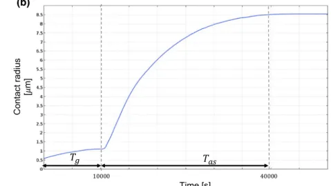
First, we validate our approach by comparing the numeri-cal results obtained for cell spreading on flat substrate with the existing literature. In this simulation, we only consider the action of the gravity, the spreading adhesive force and the contact force. The cell is initially positioned in the adhesive layer of fibronectin, but still suspended. fg and
fas are smoothly applied, and thus, they reach their maxi-mum values at Tg0= 10,000 s and Tas0= 40,000 s. As soon as the cell enters in contact with the substrate, fct applies too (Fig. 6a). In Fig. 6b, the evolution of the contact radius (i.e. the length of the cell contour in contact with the sub-strate) between the cell and the flat substrate is plotted. Gravity slightly increases the contact surface up to 1 µm. When the spreading process begins, however, we observe a much faster spreading with a maximum contact radius of 8.8 µm. This is in agreement with the experimental results presented in Cuvelier et al. (2007). The authors were able to quantify cell spreading employing reflection interfer-ence contrast microscopy (RICM) and monitoring the con-tact between the cell membrane and underneath surface. 3.2 Nucleus and cytoplasm deformation
on micropillared substrate
The second series of simulations aims at reproducing spe-cific experimental tests for which suspended cells are plated on an array of microfabricated pillars. The objective here is to analyse the nucleus and cytoplasm deformation once
the interaction between the cell and the micropillars starts and more specifically to decipher which mechanical forces play the major role and trigger the nucleus large strains. As explained in Sect. 1, the cell first settles on the pillars due to the gravity, second it slowly spreads and adheres on them,
and finally it actively deforms. This final phase may occur on the top (i.e. PAC region) or beneath (i.e. bottom region) the nucleus. Through these simulations, we would like to under-stand which of these two active strains is more relevant and promotes the nucleus self-deformation between the pillars.
Table 1 Main parameters of the
model Parameter Description Value References
cx,p x position of the cell centre in the initial configuration 0 µm cy,p y position of the cell centre in the initial configuration 8.5 µm
rc Cell radius 10 µm
rcs Cytosol radius 9.75 µm
rn Nucleus radius 5 µm
ecs Cytosol thickness 4.75 µm
em Membrane thickness 0.25 µm
ef Fibronectin layer thickness 1.5 µm
Ecp Cytoplasm Young’s modulus 100 Pa Caille et al. (2002)
En Nucleus Young’s modulus 500 Pa Fried and Johnson (1988)
𝜈c Cell’s Poisson ratio 0.485
𝜌cp Cytoplasm density 1000 kg/m3 Fried and Johnson (1988)
𝜌n Nucleus density 1400 kg/m3 Fried and Johnson (1988)
𝜇f Deviatoric viscosity 2 ×
10−3 Pa s
𝜆f Isotropic viscosity 1000 Pa s
yflat y position of the flat substrate − 2 µm yflat,l y position of the overlayer flat substrate − 6 µm xmp x position for the centre of the first pillar 8 µm
ymp y position for the centre of the first pillar − 8 µm
kmp Pillars coefficient 4.2
wmp Pillars width 8 µm
smp Inter-pillars space 8 µm
kmp,l Overlayer pillars coefficient 4.24
wmp,l Overlayer pillars width 10 µm
smp,l Overlayer inter-pillars space 8 µm
Tg Duration of the gravity phase 10,000 s
Tg0 Upper limit of Tg 10,000 s
𝜇ct Contact coefficient 2 × 10⁹ N
Tas Duration of the adhesive spreading phase 30,000 s
Tas0 Upper limit of Tas 40,000 s
𝜇as0 Focal adhesions maturation velocity 1 × 10⁶ N/s 𝜇as,max Maximum spreading coefficient 1.4 × 10⁹ N
Ta Duration of the active strain phase 10,000 s
Ta0 Upper limit of Ta 50,000 s
𝜃PAC Defining angle for the PAC domain − 18°
𝜃bottom Defining angle for the bottom domain − 35° aPAC,ext External first semi-axis of the PAC domain 10 µm bPAC,ext Internal first semi-axis of the PAC domain 9 µm aPAC,int External second semi-axis of the PAC domain 15 µm bPAC,int Internal second semi-axis of the PAC domain 14 µm ePAC Amplitude of active strain in the PAC domain 0.7 ebottom Amplitude of active strain in the bottom domain 0.7
The pillars have height kmp= 8 μm and width wmp = 8 μm and are spaced of smp= 8 μm.
In Fig. 7, the average norm of the Lagrangian deforma-tion tensor in the nucleus (Fig. 7a–c) and in the cytoplasm (Fig. 7d–f) is shown for the three scenarios: (1) ‘push’ active strain (Fig. 7a, c), (2) ‘pull’ active strain (Fig. 7b, e) and ‘push–pull’ active strain (Fig. 7c, f). For the nucleus, it is possible to notice that the strain is higher for the ‘pull’ and ‘push–pull’ configurations, with an average value of 37%. However, for the ‘push’ scenario, the nucleus only deforms of about 13%. For the cytoplasm, larger strains are achieved, especially in the region around the pillar. The cytoplasm average norm of the Lagrangian deforma-tion tensor increases from the ‘push’ configuradeforma-tion (56%) to the ‘pull’ (59%) and ‘push–pull’ (69%) configurations. In all the simulations, very large strains are observed as expected. Such an outcome completely justifies the choice of the parameters of the Yeoh material model. In fact, according to the experimental data presented in Erk et al. (2010) and Storm et al. (2005), the Young modulus of the actin fibres exponentially increases as a function of the strain. If this was the case here, the raising of the stiff-ening phenomenon would inhibit the cell penetration in between the pillars and we would not obtain the nucleus self-deformation as it has been experimentally observed (Morgan et al. 2007; Geiger et al. 2009; Liu et al. 2017, 2018). Thus, as explained in Sect. 2.1.1, the parameters 𝛼2
and 𝛼3 associated with the Yeoh visco-hyperelastic mate-rial and describing the stiffening mechanism have been kept low in our numerical model. Doing so allows to take into account the strain stiffening as described in Erk et al. (2010) and Storm et al. (2005) for strains lower than 10%, but to consider a slower increase in the cell stiffness for strains higher than 10%.
In all cases, gravity seems having little effect on the global nucleus displacement which is equal to 0.1 µm at
Tg0 . During the spreading phase (i.e. between Tg0 and Tas0 ),
the nucleus gets positioned at the beginning of the gap but is not fully engaged yet and the displacement is equal to 5 µm. During the active strain phase (i.e. between Tas0 and Ta0 ), different behaviours are observed:
• If only the PAC actively deforms (i.e. ‘push’ active strain, Fig. 8a–c, Movie 1), the maximum displacement of the nucleus is equal to 5.4 µm which corresponds to the least efficient scenario;
• If only the region beneath the nucleus deforms (i.e. ‘pull’ active strain, Fig. 8d–f, Movie 2) or if both the push and the pull forces are applied (i.e. ‘push–pull’ active strain, Fig. 8g–i, Movie 3), then the nucleus reaches 9.6 µm of displacement. Nonetheless, a slight difference can be noticed between the two cases since the combined active strains provide a nucleus displacement of 9.65 µm versus 9.63 for the pull case.
(a)
(b)
Fig. 6 a Cell spreading over a flat substrate at t = 40,000 s. b Evolution of the contact radius with respect to time between t =0 s, when the grav-ity is applied, and t = 40,000 s when the adhesion spreading force fas reaches its maximum value
(a) (b) (c)
(d)
(e) (f)
Fig. 7 a–c Average norm of the Lagrangian deformation tensor for the nucleus for the ‘push’ (a), ‘pull’ (b) and ‘push–pull’ configurations. d–f Average norm of the Lagrangian deformation tensor for the cytoplasm for the ‘push’ (a), ‘pull’ (b) and ‘push–pull’ configurations
Fig. 8 Graphical representa-tion of the numerical results for ‘push’ active strain (a–c), ‘pull’ active strain (d–f) and ‘push–pull’ active strain (g–i) (green = mem-brane, orange = cytoplasm, red = nucleus). The black lines represent the substrate and the fibronectin layer, while the blue line represents the active domain considered (a) (b) (c) (d) (e) (f) (g) (h) (i)
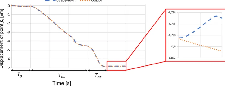
3.3 The role of gravity
According to the previous results, we can consider the ‘push and pull’ case as the control simulation since it provides the best results in terms of nucleus total displacement. We would like now to investigate the role of the gravity on the global behaviour of the cell. Pan et al. (2012) have performed a specific test which consists in putting the micropillared device upside down once the cell has spread on top of the pillars, and the nucleus has fallen between the pillars. They observed that the nucleus was deformed as significantly as on the device not overturned. To reproduce such an experi-ment, we simply ran the simulation as in Sect. 3.2, but at the end (i.e. t > Ta0 ), we inverted the sign of the gravity force
Fg. As it is possible to observe in Fig. 9, the effect of the gravity if negligible since only a difference of 0.006 µm is obtained between the control case (red curve in Fig. 9) and the ‘upside down’ case (blue curve in Fig. 9).
4 Conclusions
We presented here a computational model to investigate the mechanisms triggering nucleus self-deformation during cell spreading over a microstructured substrate. We built a 2D FE model of half of a cell which is equipped with two active domains above (i.e. the PAC) and underneath the nucleus. At the initial configuration, the cell is suspended and gently comes into contact with the pillars due to the gravity. Then, it adheres on the pillars and starts spreading and actively deforming. We have been able to discern which active strain among the ‘pushing’ in the PAC domain and the ‘pulling’ in the bottom zone is the most relevant for the
nucleus deformation. We found that PAC strain (i.e. ‘push’ active strain) has little influence on nucleus behaviour, while bottom strain (i.e. ‘pull’ active strain) alone is as efficient as the combination of both strains. Although in Hanson et al. (2015), by applying both ‘push’ and ‘pull’ forces, the nucleus was able to penetrate more deeply between the pil-lars, one may conclude that the nucleus is mostly pulled down by the actin filament that is radially distributed in the bottom region of the cell. We also tested the role of the grav-ity, and we confirmed that it has no significant impact on the nucleus strain as it has been experimentally observed by Pan et al. (2012). Our model, which includes some sophisti-cated mechanical tools (i.e. large strains, active strains and hyperelastic and viscous constitutive laws), appears to be consistent when compared to the available literature.
Nonetheless, some limitations may be drawn. First, we decided here to stick to a 2D representation for comput-ing time reasons. However, a 3D representation of the sys-tem (i.e. both the cell and the microstructured substrate) would allow to more realistically catch the cellular strains and the adaptability of the cell and of the nucleus to their environment. Second, the successive phases of the model (i.e. gravity, adhesion, spreading and active strains) are ‘user-controlled’ since they start at specific time points of the simulation. One great advance would be to let these steps depend on one or more specific biophysical quantities (Allena et al. 2013) (i.e. molecules such as globular actin or myosin) so that the system would be autoregulated. Finally, we represented the cell as an isotropic continuum and we are currently working to implement an anisotropic material model in order to take into account the critical role of the actin fibres immersed in the cytoplasm and driving, through the polymerization–depolymerization processes, the overall cell deformation (Nolan et al. 2014).
Acknowledgements This work was funded by a PhD fellowship of the French Government.
References
Abercrombie M, Heaysman JEM, Pegrum SM (1970) The loco-motion of fibroblasts in culture I. Movements of the leading edge. Exp Cell Res 59:393–398. https ://doi.org/10.1016/0014-4827(70)90646 -4
Allena R, Aubry D (2012) “Run-and-tumble” or “look-and-run”? A mechanical model to explore the behavior of a migrating amoe-boid cell. J Theor Biol 306:15–31. https ://doi.org/10.1016/j. jtbi.2012.03.041
Allena R, Mouronval A-S, Aubry D (2010) Simulation of multiple morphogenetic movements in the Drosophila embryo by a single 3D finite element model. J Mech Behav Biomed Mater 3:313–323. https ://doi.org/10.1016/j.jmbbm .2010.01.001
Allena R, Muñoz JJ, Aubry D (2013) Diffusion-reaction model for Drosophila embryo development. Comput Methods Bio-mech Biomed Eng 16:235–248. https ://doi.org/10.1080/10255 842.2011.61694 4
Ambrosi D, Pezzuto S (2011) Active stress vs. active strain in mecha-nobiology: constitutive issues. J Elast 107:199–212. https ://doi. org/10.1007/s1065 9-011-9351-4
Ambrosi D, Arioli G, Nobile F, Quarteroni A (2011) Electromechanical coupling in cardiac dynamics: the active strain approach. SIAM J Appl Math 71:605–621. https ://doi.org/10.1137/10078 8379 Badique F, Stamov DR, Davidson PM et al (2013) Directing nuclear
deformation on micropillared surfaces by substrate geometry and cytoskeleton organization. Biomaterials 34:2991–3001. https :// doi.org/10.1016/j.bioma teria ls.2013.01.018
Bao G, Suresh S (2003) Cell and molecular mechanics of biological materials. Nat Mater 2:715–725. https ://doi.org/10.1038/nmat1 001
Bell ES, Lammerding J (2016) Causes and consequences of nuclear envelope alterations in tumour progression. Eur J Cell Biol 95:449–464. https ://doi.org/10.1016/j.ejcb.2016.06.007 Benjamin M, Hillen B (2003) Mechanical influences on cells, tissues
and organs—“Mechanical Morphogenesis”. Eur J Morphol 41:3– 7.https ://doi.org/10.1076/ejom.41.1.3.28102
Bonet J, Gil AJ, Ortigosa R (2015) A computational framework for polyconvex large strain elasticity. Comput Methods Appl Mech Eng 283:1061–1094. https ://doi.org/10.1016/j.cma.2014.10.002 Caille N, Thoumine O, Tardy Y, Meister J-J (2002) Contribution of
the nucleus to the mechanical properties of endothelial cells. J Biomech 35:177–187
Cao X, Lin Y, Driscoll TP et al (2015) A chemomechanical model of matrix and nuclear rigidity regulation of focal adhesion size. Bio-phys J 109:1807–1817. https ://doi.org/10.1016/j.bpj.2015.08.048 Cherubini C, Filippi S, Nardinocchi P, Teresi L (2008) An electrome-chanical model of cardiac tissue: constitutive issues and electro-physiological effects. Prog Biophys Mol Biol 97:562–573. https ://doi.org/10.1016/j.pbiom olbio .2008.02.001
Cuvelier D, Théry M, Chu Y-S et al (2007) The universal dynamics of cell spreading. Curr Biol 17:694–699. https ://doi.org/10.1016/j. cub.2007.02.058
Davidson PM, Özçelik H, Hasirci V et al (2009) Microstructured sur-faces cause severe but non-detrimental deformation of the cell nucleus. Adv Mater 21:3586–3590. https ://doi.org/10.1002/ adma.20090 0582
Davidson PM, Fromigué O, Marie PJ et al (2010) Topographically induced self-deformation of the nuclei of cells: dependence on cell
type and proposed mechanisms. J Mater Sci Mater Med 21:939– 946. https ://doi.org/10.1007/s1085 6-009-3950-7
Davidson PM, Sliz J, Isermann P et al (2015) Design of a microflu-idic device to quantify dynamic intra-nuclear deformation during cell migration through confining environments. Integr Biol Quant Biosci Nano Macro 7:1534–1546. https ://doi.org/10.1039/c5ib0 0200a
Denais CM, Gilbert RM, Isermann P et al (2016) Nuclear envelope rupture and repair during cancer cell migration. Science 352:353– 358. https ://doi.org/10.1126/scien ce.aad72 97
Deveraux S, Allena R, Aubry D (2017) A numerical model sug-gests the interplay between nuclear plasticity and stiffness dur-ing a perfusion assay. J Theor Biol. https ://doi.org/10.1016/j. jtbi.2017.09.007
du Roure O, Saez A, Buguin A et al (2005) Force mapping in epithelial cell migration. Proc Natl Acad Sci 102:2390–2395. https ://doi. org/10.1073/pnas.04084 82102
Erk KA, Henderson KJ, Shull KR (2010) Strain stiffening in synthetic and biopolymer networks. Biomacromol 11:1358–1363. https :// doi.org/10.1021/bm100 136y
Ermis M, Akkaynak D, Chen P et al (2016) A high throughput approach for analysis of cell nuclear deformability at single cell level. Sci Rep 6:36917. https ://doi.org/10.1038/srep3 6917 Étienne J, Duperray A (2011) Initial dynamics of cell spreading are
governed by dissipation in the actin cortex. Biophys J 101:611– 621. https ://doi.org/10.1016/j.bpj.2011.06.030
Fan H, Li S (2015a) Modeling microtubule cytoskeleton via an active liquid crystal elastomer model. Comput Mater Sci 96:559–566. https ://doi.org/10.1016/j.comma tsci.2014.04.041
Fan H, Li S (2015b) Modeling universal dynamics of cell spreading on elastic substrates. Biomech Model Mechanobiol 14:1265–1280. https ://doi.org/10.1007/s1023 7-015-0673-1
Fang Y, Lai KWC (2016) Modeling the mechanics of cells in the cell-spreading process driven by traction forces. Phys Rev E 93:042404. https ://doi.org/10.1103/physr eve.93.04240 4 Fried I, Johnson AR (1988) A note on elastic energy density
func-tions for largely deformed compressible rubber solids. Comput Methods Appl Mech Eng 69:53–64. https ://doi.org/10.1016/0045-7825(88)90166 -1
Friedl P, Wolf K, Lammerding J (2011) Nuclear mechanics dur-ing cell migration. Curr Opin Cell Biol 23:55–64. https ://doi. org/10.1016/j.ceb.2010.10.015
Geiger B, Spatz JP, Bershadsky AD (2009) Environmental sensing through focal adhesions. Nat Rev Mol Cell Biol 10:21–33. https ://doi.org/10.1038/nrm25 93
Ghibaudo M, Di Meglio J-M, Hersen P, Ladoux B (2011) Mechanics of cell spreading within 3D-micropatterned environments. Lab Chip 11:805–812. https ://doi.org/10.1039/c0lc0 0221f
Golestaneh AF, Nadler B (2016) Modeling of cell adhesion and deformation mediated by receptor–ligand interactions. Biomech Model Mechanobiol 15:371–387. https ://doi.org/10.1007/s1023 7-015-0694-9
Hanson L, Zhao W, Lou H-Y et al (2015) Vertical nanopillars for in situ probing of nuclear mechanics in adherent cells. Nat Nanotechnol 10:554–562. https ://doi.org/10.1038/nnano .2015.88
Holzapfel GA (2000) Nonlinear solid mechanics: a continuum approach for engineering, 1st edn. Wiley, Hoboken
Ingber DE (2003) Tensegrity I. Cell structure and hierarchical sys-tems biology. J Cell Sci 116:1157–1173. https ://doi.org/10.1242/ jcs.00359
Jean RP, Chen CS, Spector AA (2003) Analysis of the deformation of the nucleus as a result of alterations of the cell adhesion area, pp 121–122. https ://doi.org/10.1115/imece 2003-42905
Keren K (2011) Membrane tension leads the way. Proc Natl Acad Sci 108:14379–14380. https ://doi.org/10.1073/pnas.11116 71108
Khatau SB, Hale CM, Stewart-Hutchinson PJ et al (2009) A perinu-clear actin cap regulates nuperinu-clear shape. Proc Natl Acad Sci USA 106:19017–19022. https ://doi.org/10.1073/pnas.09086 86106 Kim D-H, Khatau SB, Feng Y et al (2012) Actin cap associated focal
adhesions and their distinct role in cellular mechanosensing. Sci Rep 2:555. https ://doi.org/10.1038/srep0 0555
Kim D-H, Cho S, Wirtz D (2014) Tight coupling between nucleus and cell migration through the perinuclear actin cap. J Cell Sci 127:2528–2541. https ://doi.org/10.1242/jcs.14434 5
Liu P, Zhang YW, Cheng QH, Lu C (2007) Simulations of the spread-ing of a vesicle on a substrate surface mediated by receptor– ligand binding. J Mech Phys Solids 55:1166–1181. https ://doi. org/10.1016/j.jmps.2006.12.001
Liu X, Liu R, Gu Y, Ding J (2017) Nonmonotonic self-deformation of cell nuclei on topological surfaces with micropillar array. ACS Appl Mater Interfaces 9:18521–18530. https ://doi.org/10.1021/ acsam i.7b040 27
Liu R, Yao X, Liu X, Ding J (2018) Proliferation of cells with severe nuclear deformation on a micropillar array. Langmuir. https ://doi. org/10.1021/acs.langm uir.8b034 52
Lu H, Koo LY, Wang WM et al (2004) Microfluidic shear devices for quantitative analysis of cell adhesion. Anal Chem 76:5257–5264. https ://doi.org/10.1021/ac049 837t
Lubarda V (2004) Constitutive theories based on the multiplicative decomposition of deformation gradient: thermoelasticity, elasto-plasticity, and biomechanics. Appl Mech Rev 57:95–109 Mammoto T, Ingber DE (2010) Mechanical control of tissue and
organ development. Dev Camb Engl 137:1407–1420. https ://doi. org/10.1242/dev.02416 6
Maninova M, Caslavsky J, Vomastek T (2017) The assembly and function of perinuclear actin cap in migrating cells. Protoplasma 254:1207–1218. https ://doi.org/10.1007/s0070 9-017-1077-0 Milan J-L, Lavenus S, Pilet P et al (2013) Computational model
com-bined with in vitro experiments to analyse mechanotransduc-tion during mesenchymal stem cell adhesion. Eur Cell Mater 25:97–113
Mokbel M, Mokbel D, Mietke A et al (2017) Numerical simulation of real-time deformability cytometry to extract cell mechanical properties. ACS Biomater Sci Eng 3:2962–2973. https ://doi. org/10.1021/acsbi omate rials .6b005 58
Morgan MR, Humphries MJ, Bass MD (2007) Synergistic control of cell adhesion by integrins and syndecans. Nat Rev Mol Cell Biol 8:957–969. https ://doi.org/10.1038/nrm22 89
Muñoz JJ, Barrett K, Miodownik M (2007) A deformation gradient decomposition method for the analysis of the mechanics of mor-phogenesis. J Biomech 40:1372–1380. https ://doi.org/10.1016/j. jbiom ech.2006.05.006
Murtada S-I, Kroon M, Holzapfel GA (2010) A calcium-driven mechanochemical model for prediction of force generation in smooth muscle. Biomech Model Mechanobiol 9:749–762. https ://doi.org/10.1007/s1023 7-010-0211-0
Nisenholz N, Rajendran K, Dang Q et al (2014) Active mechanics and dynamics of cell spreading on elastic substrates. Soft Matter 10:7234–7246. https ://doi.org/10.1039/c4sm0 0780h
Nobile F, Quarteroni A, Ruiz-Baier R (2012) An active strain elec-tromechanical model for cardiac tissue. Int J Numer Methods Biomed Eng 28:52–71
Nolan DR, Gower AL, Destrade M et al (2014) A robust anisotropic hyperelastic formulation for the modelling of soft tissue. J Mech Behav Biomed Mater 39:48–60. https ://doi.org/10.1016/j. jmbbm .2014.06.016
Pan Z, Yan C, Peng R et al (2012) Control of cell nucleus shapes via micropillar patterns. Biomaterials 33:1730–1735. https ://doi. org/10.1016/j.bioma teria ls.2011.11.023
Rodriguez EK, Hoger A, McCulloch AD (1994) Stress-dependent finite growth in soft elastic tissues. J Biomech 27:455–467 Rosenbluth MJ, Lam WA, Fletcher DA (2008) Analyzing cell
mechanics in hematologic diseases with microfluidic bio-physical flow cytometry. Lab Chip 8:1062–1070. https ://doi. org/10.1039/b8029 31h
Sarvestani AS, Jabbari E (2008) Modeling the kinetics of cell membrane spreading on substrates with ligand density gradi-ent. J Biomech 41:921–925. https ://doi.org/10.1016/j.jbiom ech.2007.11.004
Sauer RA (2016) A survey of computational models for adhe-sion. J Adhes 92:81–120. https ://doi.org/10.1080/00218 464.2014.10032 10
Schirmer EC, de las Heras JI (eds) (2014) Cancer biology and the nuclear envelope: recent advances may elucidate past paradoxes. Springer, New York
Stålhand J, Klarbring A, Holzapfel GA (2008) Smooth muscle contraction: mechanochemical formulation for homogeneous finite strains. Prog Biophys Mol Biol 96:465–481. https ://doi. org/10.1016/j.pbiom olbio .2007.07.025
Storm C, Pastore JJ, MacKintosh FC et al (2005) Nonlinear elasticity in biological gels. Nature 435:191–194. https ://doi.org/10.1038/ natur e0352 1
Swift J, Ivanovska IL, Buxboim A et al (2013) Nuclear lamin-A scales with tissue stiffness and enhances matrix-directed dif-ferentiation. Science 341:1240104. https ://doi.org/10.1126/ scien ce.12401 04
Tan JL, Tien J, Pirone DM et al (2003) Cells lying on a bed of microneedles: an approach to isolate mechanical force. Proc Natl Acad Sci USA 100:1484–1489. https ://doi.org/10.1073/ pnas.02354 07100
Versaevel M, Grevesse T, Gabriele S (2012) Spatial coordination between cell and nuclear shape within micropatterned endothelial cells. Nat Commun 3:671. https ://doi.org/10.1038/ncomm s1668 Wang H, Biao Y, Chunlai Y, Wen L (2017) Simulation of AFM inden-tation of soft biomaterials with hyperelasticity. In: 2017 IEEE 12th international conference on nano/micro engineered and molecular systems (NEMS), pp 550–553
Wolf K, Te Lindert M, Krause M et al (2013) Physical limits of cell migration: control by ECM space and nuclear deformation and tuning by proteolysis and traction force. J Cell Biol 201:1069– 1084. https ://doi.org/10.1083/jcb.20121 0152
Yeoh OH (1993) Some forms of the strain energy function for rubber. Rubber Chem Technol 66:754–771. https ://doi. org/10.5254/1.35383 43
Zeng X, Li S (2011a) Modelling and simulation of substrate elasticity sensing in stem cells. Comput Methods Biomech Biomed Eng 14:447–458. https ://doi.org/10.1080/10255 842.2011.55737 1 Zeng X, Li S (2011b) Multiscale modeling and simulation of soft
adhesion and contact of stem cells. J Mech Behav Biomed Mater 4:180–189. https ://doi.org/10.1016/j.jmbbm .2010.06.002 Zeng X, Li S (2012) A three dimensional soft matter cell model for
mechanotransduction. Soft Matter 8:5765–5776. https ://doi. org/10.1039/c2sm0 7138j