arXiv:1101.5620v2 [astro-ph.EP] 3 Jun 2011
Thermal emission at 4.5 and 8 µm of WASP-17b, an
extremely large planet in a slightly eccentric orbit
D. R. Anderson,
1⋆A. M. S. Smith,
1A. A. Lanotte,
2T. S. Barman,
3A. Collier Cameron,
4C. J. Campo,
5M. Gillon,
2J. Harrington,
5C. Hellier,
1P. F. L. Maxted,
1D. Queloz,
6A. H. M. J. Triaud,
6P. J. Wheatley
71Astrophysics Group, Keele University, Staffordshire ST5 5BG, UK
2Institut d’Astrophysique et de G´eophysique, Universit´e de Li`ege, All´ee du 6 Aoˆut, 17, Bat. B5C, Li`ege 1, Belgium 3Lowell Observatory, 1400 West Mars Hill Road, Flagstaff, AZ 86001, USA
4SUPA, School of Physics and Astronomy, University of St. Andrews, North Haugh, Fife, KY16 9SS, UK 5Planetary Sciences Group, Department of Physics, University of Central Florida, Orlando, FL 32816-2385, USA 6Observatoire de Gen`eve, Universit´e de Gen`eve, 51 Chemin des Maillettes, 1290 Sauverny, Switzerland
7Department of Physics, University of Warwick, Coventry, CV4 7AL, UK
Accepted 1988 December 15. Received 1988 December 14; in original form 1988 October 11
ABSTRACT
We report the detection of thermal emission at 4.5 and 8 µm from the planet WASP-17b. We used Spitzer to measure the system brightness at each wavelength during two occultations of the planet by its host star. By combining the resulting light curves with existing transit light curves and radial velocity measurements in a simultaneous analysis, we find the radius of WASP-17b to be 2.0 RJup, which is 0.2 RJuplarger than
any other known planet and 0.7 RJup larger than predicted by the standard cooling
theory of irradiated gas giant planets. We find the retrograde orbit of WASP-17b to be slightly eccentric, with 0.0012 < e < 0.070 (3 σ). Such a low eccentricity suggests that, under current models, tidal heating alone could not have bloated the planet to its current size, so the radius of WASP-17b is currently unexplained. From the measured planet-star flux-density ratios we infer 4.5 and 8 µm brightness temperatures of 1881 ± 50 K and 1580 ± 150 K, respectively, consistent with a low-albedo planet that efficiently redistributes heat from its day side to its night side.
Key words: methods: data analysis – techniques: photometric – occultations – plan-ets and satellites: atmospheres – planplan-ets and satellites: individual: WASP-17b – stars: individual: WASP-17 – planetary systems – infrared: planetary systems.
1 INTRODUCTION
WASP-17b is a transiting, 0.49-Jupiter-mass planet in a 3.74-day orbit around a metal-poor, 1.3-Solar-mass F6V star (Anderson et al. 2010b, hereafter A10). Data presented in A10, confirmed by Triaud et al. (2010, hereafter T10) and Bayliss et al. (2010), indicated that WASP-17b is in a ret-rograde orbit around its host star, the first such orbit to be found.
WASP-17b probably formed beyond the ice line in a near-circular, coplanar orbit, as predicted by the canon-ical model of star and planet formation. It may have subsequently acquired an eccentric, highly inclined or-bit via planet-planet scattering (e.g. Ford & Rasio 2008) or the Kozai mechanism (e.g. Fabrycky & Tremaine 2007;
Nagasawa, Ida & Bessho 2008). Tidal friction may then have shortened and circularised the long, eccentric orbit, with the energy being dissipated within the planet as heat (e.g. Jackson, Greenberg & Barnes 2008b; Ibgui & Burrows 2009).
As the planet is low-mass and the star is hot (Teff =
6650 ± 80K, T10) and fast-rotating (v sin I = 9.8 km s−1,
T10), the radial velocity (RV) measurements are relatively low signal-to-noise, and so the eccentricity of the planet’s orbit was poorly constrained (e = 0–0.24) in the discovery paper (A10). This translated into uncertainties in the stellar radius (R∗= 1.2–1.6 R⊙) and thus in the planetary radius
(Rpl= 1.5–2.0 RJup), meaning the planet is larger than
pre-dicted by the standard cooling theory of irradiated gas giant planets by 0.2–0.7 RJup(Fortney, Marley & Barnes 2007).
Using a coupled radius-orbit evolutionary model, Ibgui & Burrows (2009) demonstrated that planets can be
inflated to radii of 2 RJup and beyond during a transient
phase of heating that accompanies the tidal circularisation of a short (a ≈ 0.1 AU), highly eccentric (e ≈ 0.8) orbit. Such a large radius persists for only a few tens of Myr, sug-gesting that we are unlikely to observe any one system dur-ing this brief stage. However, only 3–4 of the ∼100 known planets are extremely bloated and the transit technique does preferentially find large planets.
Leconte et al. (2010) argued that the tidal heating rate is underestimated for even moderately eccentric orbits in studies such as that of Ibgui & Burrows (2009). If true, then a large fraction of energy tidally dissipated within the planet would have been radiated away by the age typical of the most bloated planets (a few Gyr) and so could not have played a significant role in their observed bloating. Ibgui, Spiegel & Burrows (2011) admit that their equations are not applicable at large eccentricity, but counter that nei-ther are those that Leconte et al. (2010) use. They state that the current uncertainty in tidal theory means that no approach can be considered correct.
In A10, the derived radius of WASP-17b is largest (2.0 RJup) when a circular orbit is imposed, smaller
(1.7 RJup) when eccentricity is a free parameter (e =
0.13), and smaller again (1.5 RJup) when a
main-sequence prior is imposed on the star and eccentric-ity is let free (e = 0.24). Ibgui & Burrows (2009) and Ibgui, Spiegel & Burrows (2011) each note that, compared to planets that did not undergo tidal heating, tidally in-flated planets are still signicantly larger Gyr after their or-bits have circularised and tidal heating has ceased. In each study though, the orbits are still significantly non-circular (e & 0.1) when the planets are largest. Hence, if the or-bit of WASP-17b were found to be near-circular (which would mean that Rpl≈ 2 RJup) then it would seem unlikely
that the planet could have been inflated by a single episode of tidal inflation. Another possibility is an ongoing tidal heating scenario, as explored by Ibgui, Burrows & Spiegel (2010), in which the orbit of WASP-17b would be kept non-circular by the continuing interaction with an as-yet undis-covered third body.
In order to better constrain the stellar and planetary radii, the system age, and the potential transient and ongo-ing tidal heatongo-ing rates, an improved determination of orbital eccentricity is required. Further high-precision RV measure-ments were obtained and presented in T10. These allowed eccentricity to be better constrained to e = 0.066+0.030
−0.043. The
best prospect of improving this situation further lay with the measurement of an occultation (as the planet passes behind the star), which would constrain e cos ω, where ω is the ar-gument of periastron.
In addition, by observing occultations from the ground (e.g. Anderson et al. 2010a) and from space (e.g. Wheatley et al. 2010), we are able to perform photometry and emission spectroscopy of exoplanets which are spatially unresolved from their host stars. This allows us to deter-mine planet albedos and the rates at which energy is redis-tributed from the day side to the night side of the planet (e.g. Barman 2008), and to infer the temperature structure (e.g. Knutson et al. 2008) and chemical composition of planet at-mospheres (e.g. Swain et al. 2009).
We present here observations of two occultations of WASP-17b, each of which was measured at both 4.5 and
8 µm. We combine these new data with existing data in a simultaneous analysis to show that WASP-17b is the largest (Rpl = 2.0 RJup) and least-dense (ρpl = 0.06 ρJup) planet
known, and is in a slightly eccentric orbit around a 2–3 Gyr-old, F-type star. Exoplanet occultation photometry is at the limit of Spitzer systematics and reliable conclusions concerning atmospheres and orbits depend on a careful anal-ysis of the data. We thus present a detailed description of our method.
2 NEW OBSERVATIONS
We observed two occultations of the planet WASP-17b by its Ks = 10.22 host star with the Spitzer Space Telescope
(Werner et al. 2004) during 2009 April 24 and 2009 May 1. On each date we measured the WASP-17 system with the Infrared Array Camera (IRAC, Fazio et al. 2004) in full ar-ray mode (256 × 256 pixels, 1.2 arcsec/pixel) simultaneously in channel 2 (4.5 µm) and channel 4 (8 µm) for a duration of 8.4 hr. We used an effective integration time of 10.4 s, resulting in 2319 images per channel per occultation. To reduce the time-dependent sensitivity of the 8 µm channel (e.g. Knutson et al. 2008), we exposed the array to a bright, diffuse source (M42) for 214 frames immediately prior to each occultation observation.
We used the images calibrated by the standard Spitzer pipeline (version S18.7.0) and delivered to the community as Basic Calibrated Data (BCD). We added back to each image the estimated brightness of the zodiacal light in the sky dark (Reach et al. 2005) so photometric uncertainties and the op-timal aperture radii are correctly determined. For each im-age, we converted flux from MJy sr−1to electrons and then
used iraf to perform aperture photometry for WASP-17, using circular apertures with a range of radii (1–6 pixels). The apertures were centred by fitting a Gaussian profile on the target. The sky background was measured in an annu-lus extending from 8 to 12 pixels from the aperture centre, and was subtracted from the flux measured within the on-source apertures. We estimated the photometric uncertainty as the quadrature addition of the uncertainty in the sky background in the on-source aperture, the read-out noise, and the Poisson noise of the total background-subtracted counts within the on-source aperture. We calculated the mid-exposure times in the HJD (UTC) time system from the MHJD OBS header values, which are the start times of the DCEs (Data Collection Events), by adding half the integration time (FRAMTIME) values.
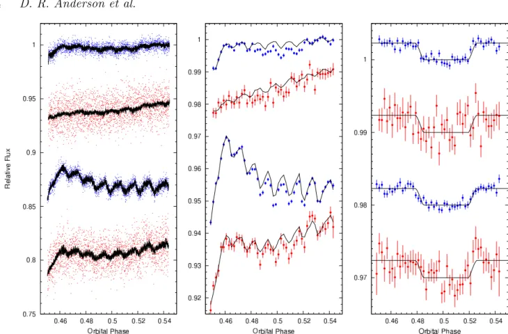
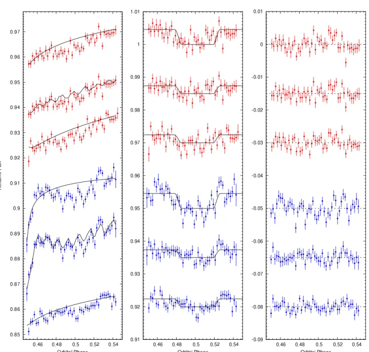
We found (see Section 3) that for WASP-17 the highest signal-to-noise is obtained when using an aperture radius of 2.9 pixels for the 4.5 µm data, and a radius of 1.6 pixels for the 8 µm data. The data are displayed raw and binned in the first and second panels, respectively, of Figure 1.
We rejected any flux measurement that was discrepant with the median of its 20 neighbours (a window width of 4.4 min) by more than four times its theoretical error bar. We also performed a rejection on target position. For each image and for the x and y detector coordinates separately, we computed the difference between the fitted target posi-tion and the median of its 20 neighbours. For each dataset, we then calculated the standard deviation σ of these me-dian differencesand rejected any points discrepant by more
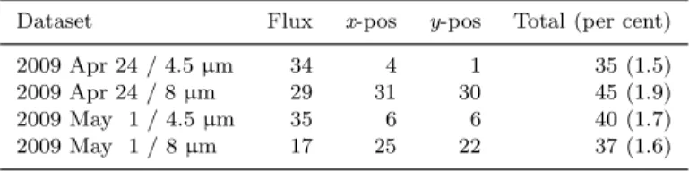
Table 1.Number of points rejected per dataset per criterion.
Dataset Flux x-pos y-pos Total (per cent)
2009 Apr 24 / 4.5 µm 34 4 1 35 (1.5)
2009 Apr 24 / 8 µm 29 31 30 45 (1.9)
2009 May 1 / 4.5 µm 35 6 6 40 (1.7)
2009 May 1 / 8 µm 17 25 22 37 (1.6)
than 4 σ. The numbers of points rejected on flux and target position for each dataset are given in Table 1.
According to the IRAC handbook, each IRAC array receives approximately 1.5 solar-proton and cosmic-ray hits per second, with ∼2 pixels affected in channel 2, and ∼6 pixels per hit affected in channel 4, while the cosmic ray flux varies randomly by up to a factor of a few over time-scales of minutes. Thus the probability per exposure that pixels within the stellar aperture will be affected by a cosmic ray hit is 1.5 per cent for channel 2 and 1.3 per cent for channel 4, which is in good agreement with the small portion of frames that we rejected.
3 DATA ANALYSIS 3.1 Data and model
We determined the system parameters from a simultaneous analysis incorporating: our new Spitzer occultation photom-etry; the WASP discovery photometry covering the full or-bit for the three seasons (March to August) of 2006–2008 and presented in A10; a high-precision, Ic-band transit light
curve taken with the 1.2-m Euler-Swiss telescope on 2008 May 6 and presented in A10; and 124 RV measurements, including 34 taken during transit, made with the CORALIE and HARPS spectrographs and presented in A10 and T10.
These data were input into an adaptive Markov-chain Monte Carlo (MCMC) algorithm (Collier Cameron et al. 2007; Pollacco et al. 2008; Enoch et al. 2010). Such a simul-taneous analysis is necessary to take account of the cross-dependency of system parameters and to make an hon-est assessment of their uncertainties. We used the follow-ing as MCMC proposal parameters: Tc, P , ∆F , T14, b, K1,
Teff, [Fe/H],√e cos ω,√e sin ω,
√
v sin I cos λ,√v sin I sin λ, ∆F4.5µm and ∆F8µm (see Table 5 for definitions).
At each step in the MCMC procedure, each proposal parameter is perturbed from its previous value by a small, random amount. Stellar density, which is constrained by the shape of the transit light curve (Seager & Mall´en-Ornelas 2003) and the eccentricity of the orbit, is calculated from the proposal parameter values. This is input, together with the latest values of Teff and [Fe/H] (which are controlled
by Gaussian priors) into the empirical mass calibration of Enoch et al. (2010) to obtain an estimate of the stellar mass M∗. From the proposal parameters, model light and RV
curves are generated and χ2 is calculated from their
com-parison with the data. A step is accepted if χ2 (our merit
function) is lower than for the previous step, and a step with higher χ2 is accepted with probability exp(−∆χ2/2). In this way, the parameter space around the optimum so-lution is thoroughly explored. The value and uncertainty of
each parameter are respectively taken as the median and central 68.3 per cent confidence interval of the parameter’s marginalised posterior probability distribution.
As Ford (2006) notes, it is convenient to use e cos ω and e sin ω as MCMC proposal parameters, because these two quantities are nearly orthogonal and their joint probabil-ity densprobabil-ity function is well-behaved when the eccentricprobabil-ity is small and ω is highly uncertain. Ford cautions, however, that the use of e cos ω and e sin ω as proposal parameters implicitly imposes a prior on the eccentricity that increases linearly with e. As such, we instead use√e cos ω and√e sin ω as proposal parameters, which restores a uniform prior on e. For similar reasons, we use√v sin I cos λ and√v sin I sin λ rather than v sin I cos λ and v sin I sin λ to parameterise the Rossiter-McLaughlin effect (e.g. Gaudi & Winn 2007).
3.2 Spitzer data
3.2.1 Deciding between models and datasets
Systematics are present in IRAC photometry at a level simi-lar to the predicted planetary occultation signal. Therefore, it is necessary to carefully detrend the photometry so as to obtain accurate occultation depths and timings. To dis-criminate between various detrending models we used the Bayesian Information Criterion (BIC, Schwarz 1978): BIC = χ2+ k ln N (1) where k is the number of free model parameters and N is the number of data-points. The BIC prefers simpler models unless the addition of extra terms significantly improves the fit. As such, it is a useful tool for selecting between models with different numbers of free parameters.
In addition, we used the root mean square (RMS) of the residuals about the best-fitting trend and occultation models to discriminate between different light curves obtained from different reductions of the same sets of images.
3.2.2 Aperture radii
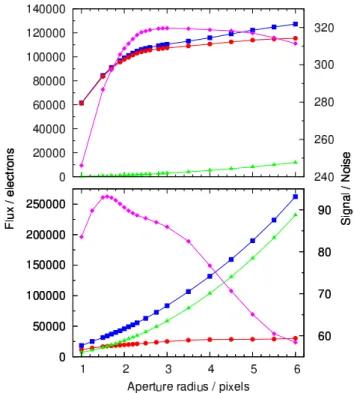
We determined the optimal aperture radii to use for the 4.5 and 8 µm data by performing aperture photometry with a range of aperture radii (1–6 pixels), and choosing the radii that produced the maximal signal-to-noise (Figure 2; e.g. Howell 1989).
For the 4.5 µm data, the radius that results in the high-est signal-to-noise is 2.9 pixels and it is this radius that we adopt (Figure 2, upper panel). This radius incorporates the majority (∼92.5 per cent) of the target flux and little back-ground flux (∼2.6 per cent of that of the target).
At 8 µm, as compared to 4.5 µm, the background is brighter by a factor ∼20 and the source is fainter by a fac-tor ∼4. Thus, with increasing aperture radius, the back-ground flux quickly dominates the target flux (Figure 2, lower panel). Indeed, the background flux equals the tar-get flux when using our adopted, optimal (highest signal-to-noise) radius of only 1.6 pixels. This radius incorporates ∼60 per cent of the target flux and a similar amount (97 per cent of the target) of background flux. The background flux is greater than the target flux by factors of approximately 1.5, 2, 3 and 7.5 within apertures with radii of 2.2, 2.75, 3.5 and 6 pixels respectively.
Figure 1. In each of the above three plots, the upper two datasets were obtained at 4.5 µm (blue) and 8 µm (red) on 2009 April 24 and the lower two datasets were taken at 4.5 µm (blue) and 8 µm (red) on 2009 May 1. Relative flux offsets were applied to datasets for clarity. Left: Raw Spitzer data with the best-fitting trend and occultation models superimposed. Middle: The same data binned in phase (∆φ = 0.002, ∼11 min) with the best-fitting trend models superimposed. Right: The binned data after dividing by the best-fitting trend models, and with the best-fitting occultation models superimposed. We normalise the flux received from the star alone to unity, which is measured during occultation.
3.2.3 Systematics
IRAC uses an InSb detector to detect light around 4.5 µm, and the measured flux exhibits a strong correlation with the position of the target star on the array. This effect is due to the inhomogeneous intra-pixel sensitivity of the detector and is well-documented (e.g. Knutson et al. 2008, and references therein). Following Charbonneau et al. (2008) we modelled this effect as a quadratic function of the sub-pixel position of the PSF centre, but with the addition of a linear term in time:
df = a0+ axdx + aydy + axxdx2+ ayydy2+ atdt (2)
where df = f − ˆf is the stellar flux relative to its weighted mean, dx = x − ˆx and dy = y − ˆy are the coordinates of the PSF centre relative to their weighted means, dt is the time since the beginning of the observation, and a0,
ax, ay, axx, ayy and at are coefficients. We determined the
trend model coefficients by linear least-squares minimiza-tion at each MCMC step, subsequent to division of the data by the eclipse model. We used singular value decomposi-tion (Press et al. 1992) for this purpose. Though a common eclipse model was fitted to occultation data from the same channel, trend models were fitted separately to each dataset. The best-fitting trend models are superimposed on the binned photometry in the middle panel (first and third curves from the top) of Figure 1. Table 2 gives the
best-Table 2.Trend model parameters and coefficients
4.5 µm 8 µm
2009 Apr 24 2009 May 1 2009 Apr 24 2009 May 1 ˆ f 106955.09 107395.47 17289.49 17866.66 ˆ x 24.28 24.85 25.23 25.64 ˆ y 25.28 25.44 23.02 23.18 a0 −26.0+3.6−3.8 −10.8 +10.7 −10.4 −108.42 +0.67 −0.77 −94.2 +3.1 −3.1 ax −2606.7+13.1−13.3 4927.2 +61.1 −60.5 720.2 +6.5 −6.2 −142.0 +19.1 −20.1 ay −5049.5+20.2−20.3 −6866.5 +11.9 −11.6 42.3 +5.2 −4.9 −1301.6 +7.7 −7.2 axx 8345.6+479.7−487.6 −105.0−661.9+636.2 −1368.7+114.6−110.7 −1748.4+401.7−398.4 ayy −8340.8+385.5−416.0 3663.4 +155.7 −165.5 −1246.8 +136.0 −134.3 905.4 +122.2 −121.2 at 207.7+20.7−19.2 −14.5 +35.8 −37.0 648.9 +5.2 −4.9 557.7 +9.0 −9.1
fitting values for the trend model parameters (Equation 2), together with their 1-σ uncertainties.
We found consistent 4.5 µm eclipse depths when in-corporating one of the two datasets or both of them in our analysis: ∆F4.5µm1 = 0.00225 ± 0.00015, ∆F4.5µm2 =
0.00244 ± 0.00020, and ∆F4.5µm1+2= 0.00230 ± 0.00012.
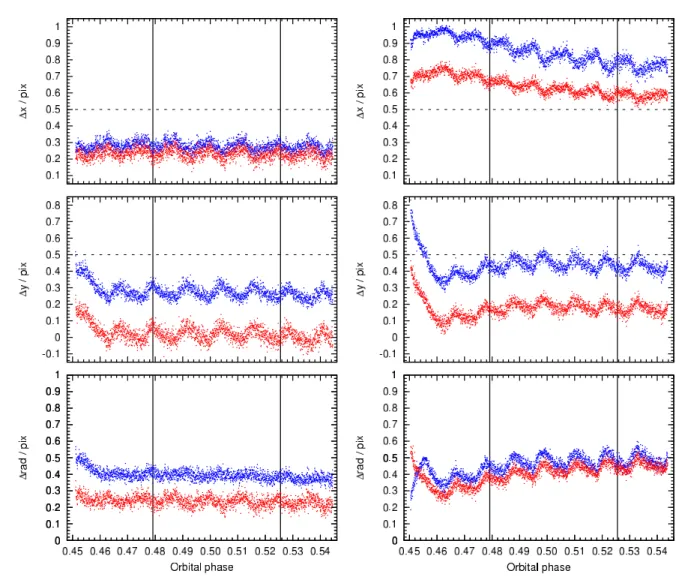
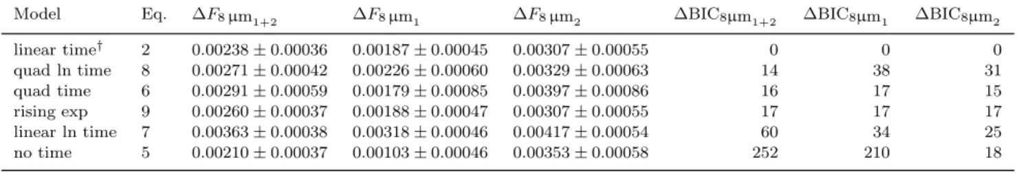
The systematics in the data from 2009 April 24 are of much smaller amplitude than those in the data from 2009 May 1. This is due to a chance placement of the target star on the detector. The detector positions of WASP-17’s PSF centre are shown in Figure 3. During each occultation and
Figure 2. The flux due to WASP-17 (red circles), the sky and instrumental background (green triangles), and both WASP-17 and the background combined (blue squares), as well as the signal-to-noise (magenta diamonds) as a function of aperture radius. The upper and lower panels show the 4.5 µm and 8 µm data respectively. We show the data from 2009 Apr 24, but the data from 2009 May 1 produce near-identical plots.
in each channel the motion due to the nodding of the space-craft is evident in the x and y positions of the PSF centres. However, contrasting the two occultations, there is a marked difference in the radial distance from the nearest pixel centre over the course of the observations. In the data from 2009 Apr 24 the placement of the target on the detectors is such that the motion of the spacecraft in the x-direction largely compensates for the motion in the y-direction, resulting in a near constant radial distance from the nearest pixel centre. The opposite is the case in the 2009 May 1 dataset, where the motion in the x and y directions combines to produce large-amplitude oscillations in the distance from the nearest pixel centre. This results in the large saw-tooth systematics seen in the light curve (second panel of Figure 1).
Near the beginning of the observations on 2009 May 1, the target crossed a pixel boundary on the 4.5 µm detector (Figure 3, middle-right plot). This resulted in a point of inflection in the distance of the target from the nearest pixel centre (Figure 3, bottom-right plot). As the sensitivity is higher toward the pixel centre and lower near the edges, it is therefore curious that no corresponding inflection point is seen in the light curve (Figure 1, middle panel).
IRAC uses a SiAs detector to observe at 8 µm, and its response is usually thought to be homogeneous, though another systematic affects the photometry. This effect is known as the ‘ramp’ because it causes the gain to in-crease asymptotically over time for every pixel, with an amplitude depending on a pixel’s illumination history (e.g. Knutson et al. 2008, and references therein). Again
follow-ing Charbonneau et al. (2008), we modelled this ramp as a quadratic function of ln(dt):
df = a0+ a1ln(dt + toff) + a2(ln(dt + toff))2 (3)
where toffis a proposal parameter. To prevent tofffrom
drift-ing more than an hour or so prior to the first observation, we place on it a Gaussian prior by adding a Bayesian penalty to our merit function (χ2):
BPtoff= t
2 off/σ
2
toff (4)
where σtoff = 15 min.
From an initial MCMC run, we observed systematics in the residuals of the second 8 µm dataset, and so investi-gated decorrelating the 8 µm data with detector position. A significantly lower occultation BIC (∆BIC = −141) resulted when also detrending for detector position, i.e. detrending with Equation 2 rather than with Equation 3. In addition, there was less scatter in the 8 µm data when decorrelating with detector position (i.e. when detrending with Equation 2 rather than with Equation 3; Figure 4 and Table 3). When not decorrelating with detector position, significantly dif-ferent best-fitting 8 µm occultation depths were obtained for the two individual datasets (Table 3) and the depth ob-tained from the combined datasets was much deeper than otherwise. For these reasons and for reasons that will be pre-sented in the remainder of this section, we opted to decor-relate the 8 µm data with detector position.
In Section 3.3 we use deconvolution photometry to show that the observed dependence on detector position is likely to have been introduced during aperture photometry. Thefore there is no evidence of an inhomogeneous intrapixel re-sponse of the SiAs 8 µm detector, contrary to the case with the InSb 4.5 µm detector.
The second and fourth curves from the top in the middle panel of Figure 1 are the best-fitting trend models when detrending the two 8 µm datasets with Equation 2. Note that the saw-tooth patterns of the 8 µm trend models are in phase with those of the 4.5 µm trend models, though each dataset was fit separately with its own trend model.
In addition to Equation 2, which we will call lin-ear time, we tried trend functions with a variety of time-dependency. These were no time:
df = spatial (5)
where spatial = a0+ axdx + aydy + axxdx2+ ayydy2
repre-sents the detector position terms and an offset; quad time: df = spatial + atdt + attdt2; (6)
linear ln time:
df = spatial + a1ln(dt + toff); (7)
quad ln time:
df = spatial + a1ln(dt + toff) + a2(ln(dt + toff))2; (8)
and rising exp (Harrington et al. 2007):
df = spatial + a3exp(a4dt). (9)
where a4 is a proposal parameter.
In Table 4 we present the occultation depths and BIC values resulting from detrending the 8 µm data with the various models. The 4.5 and 8 µm data were fitted simul-taneously, so an improved fit to the 8 µm data would not
Figure 3.The detector positions of WASP-17’s PSF centre for the first occultation (left-hand plots) and the second occultation (right-hand plots). The PSF centre positions on the 4.5 and 8 µm detectors are respectively depicted by blue and red dots. For each occultation we show the distance of the PSF centre from the nearest pixel centre in the x and y directions (top and middle panels respectively) and in the radial direction (bottom panels). Pixel centres are located at (x, y) = (0, 0) while pixel edges are located at (0.5, 0.5) and are demarcated by dashed lines.
Table 3.A comparison of the 8 µm occultation depths and residuals from deconvolution photometry and aperture photometry.
Method Trend eq. ∆F8µm1+2 ∆F8µm1 ∆F8µm2 RMS8µm1+2 RMS8µm1 RMS8µm2
aper. phot. 2 0.00238 ± 0.00036 0.00187 ± 0.00050 0.00303 ± 0.00059 0.01103 0.01142 0.01010 aper. phot. 3 0.00455 ± 0.00036 0.00246 ± 0.00058 0.00643 ± 0.00055 0.01112 0.01127 0.01119 decon. phot. 3 0.00240 ± 0.00036 0.00202 ± 0.00052 0.00276 ± 0.00047 0.00994 0.01019 0.00967
be preferred if the fit to the 4.5 µm data were considerably worse. In Table 4 the models are presented in descending or-der by how well they fit the combined 8 µm datasets, and the BIC values are given relative to the best-fitting model (lin-ear time). The lin(lin-ear time model is strongly favoured and we thus adopt this as our trend model for the 8 µm data. The BIC values resulting from MCMC runs incorporating the two 8 µm datasets individually (8µm1 and 8µm2) are also given, with a similar order of preference to that of the combined datasets. Again, the linear time model is clearly favoured over the others, supporting our decision to use the same model for the two datasets. The occultation depths are
consistent between the four most preferred models, but are not so for the two less preferred models. The depths found from the first dataset are shallower than those found from the second dataset, with a difference between the two of 1.7σ in the case of the linear time trend model.
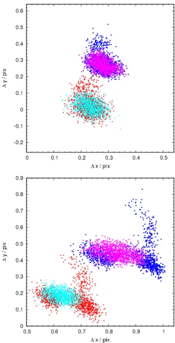
In Figure 5 we present the detector positions of WASP-17 both during and outside of occultation. On 2009 Apr 24, the star occupied the same region of the detector during the occultation as when outside of occultation. However, on 2009 May 1, the star occupied different regions of the detector during occultation than when outside of occultation, though there was some overlap. The reason for this can be seen
Figure 4. A comparison of the methods for reducing and detrending the 8 µm data. In each of the above three panels, the upper three curves (red dots) are the data from 2009 Apr 24 and the lower three curves (blue dots) are the data from 2009 May 1. In each triplet of curves, the top curve is the light curve obtained by aperture photometry and detrended with Equation 3. The middle curve is the light curve obtained by aperture photometry and detrended with Equation 2. The bottom curve is the light curve obtained by deconvolution photometry and detrended with Equation 3. Left panel: Binned raw data, with the best-fitting trend models superimposed. Middle panel: Binned detrended data, with the best-fitting occultation models superimposed. Right panel: Binned residuals about the best-fitting trend and occultation models.
in the top-right panel of Figure 3, which shows that the star moved steadily in the x-direction. This was in addition to the motion due to the nodding of the spacecraft, which resulted in some overlap between the in-occultation and out-of-occultation detector positions. As we decorrelate the light curves with detector position, the data from 2009 Apr 24, with the greater detector position overlap, are thought to be more reliable. However, the data from the two occultations detrend similarly well, and we find no reason to disregard the latter dataset.
This indicates that, though we had requested the same detector positions for the target for each observation run, small differences in the pointing and motion of Spitzer can result in markedly different systematics.
We investigated using the fitted PSF positions from the higher signal-to-noise 4.5 µm data in the aperture photome-try and positional decorrelation of the 8 µm data. To account for the offset between the two detectors we fit the differences in the x and y directions and translated the coordinates by those amounts. The 8 µm occultation depths, both when in-corporating one of the two datasets or both of them, were
Table 4.The 8-µm occultation depths and the combined (4.5 and 8 µm) relative occultation BIC values, when detrending the 8 µm data with the various models
Model Eq. ∆F8µm1+2 ∆F8µm1 ∆F8µm2 ∆BIC8µm1+2 ∆BIC8µm1 ∆BIC8µm2
linear time† 2 0.00238 ± 0.00036 0.00187 ± 0.00045 0.00307 ± 0.00055 0 0 0 quad ln time 8 0.00271 ± 0.00042 0.00226 ± 0.00060 0.00329 ± 0.00063 14 38 31 quad time 6 0.00291 ± 0.00059 0.00179 ± 0.00085 0.00397 ± 0.00086 16 17 15 rising exp 9 0.00260 ± 0.00037 0.00188 ± 0.00047 0.00307 ± 0.00055 17 17 17 linear ln time 7 0.00363 ± 0.00038 0.00318 ± 0.00046 0.00417 ± 0.00054 60 34 25 no time 5 0.00210 ± 0.00037 0.00103 ± 0.00046 0.00353 ± 0.00058 252 210 18
†For linear time: BIC
4.5µm1+2+8µm1+2= 10 772, BIC4.5µm1+2+8µm1= 8 298 and BIC4.5µm1+2+8µm2= 8 072.
very similar to those obtained when fitting the stellar PSF position in the 8 µm data, and there was no significant re-duction in the residual scatter about the best-fitting models. Hence, we proceeded as before.
Spitzer’s pointing oscillates around the nominal posi-tion, with an amplitude of ∼0.1 pixels over a period of ∼1 hour. We also see higher frequency jitter, with periods of 1–2 minutes (the cadence of our data is 12 seconds), in the posi-tion of WASP-17. Some authors (e.g. Wheatley et al. 2010) chose to smooth the measured target positions prior to light curve detrending. However, we found that detrending with the unsmoothed positions resulted in a reduced BIC (∆BIC = −931), and in smaller residual RMS values: 5.3 and 8.8 per cent lower for the two 4.5 µm datasets, and 0.6 and 1.4 per cent lower for the two 8 µm datasets.
To ascertain whether the observed short-period jitter was due to measurement error, we measured the position of a second star in the field for the two 4.5 µm datasets. For both WASP-17 and the second star we subtracted their Gaussian-smoothed (σ = 84 s) positions to remove the longer-period oscillations. We then fitted Gaussians to the distributions of the detector x and y coordinates of both stars and of their relative separations. If the measured positions of WASP-17 and the second star are uncorrelated, then the variance of the distribution of relative separations would be the sum of the variances of the distributions of each star’s positions. However, we found that the distribution of separation in the x-direction had a variance smaller than that by a factor nine for the first dataset and by a factor two for the second dataset. For the y-coordinate, the factors were 25 and 6 for the two datasets. Thus, the short-period jitter is real and the light curves should be detrended with unsmoothed target positions.
3.2.4 Aperture radii revisited
As a check of the choice of aperture radius (2.9 pixels) for the 4.5 µm data, we input the 4.5 µm light curves obtained with each aperture radius into a simultaneous MCMC analysis that incorporated all but the 8 µm data. These analyses produced consistent 4.5 µm occultation depths (Figure 6, upper panel), indicating that the 4.5 µm result is relatively insensitive to the choice of aperture radius.
As a check of the choice of aperture radius (1.6 pix-els) for the 8 µm data, we input each 8 µm light curve into a simultaneous MCMC analysis that incorporated all other data. When decorrelating with detector position (Fig-ure 6, middle panel), the fitted 8 µm occultation depth varies
weakly with aperture radius. Beyond an aperture radius of 3.5 pixels (by which point the flux due to the sky background is 3 times that of the target within the target aperture), a deeper occultation is measured. Without decorrelating with detector position (Figure 6, lower panel), the fitted 8 µm occultation depth is a strong function of aperture radius.
As the conclusions drawn from Spitzer occultation observations depend on accurately measured occultation depths, we advise others to check for a correlation between flux and detector position in their 5.8 µm and 8 µm datasets, and for a dependence of occultation depth on aperture ra-dius. For example, from Figure 1 of Fressin et al. (2010) it appears that similar patterns of saw-tooth systematics are present in both the 4.5 and 8 µm light curve, though they only decorrelate the former light curve with detector posi-tion. If a dependence of measured flux on detector position was introduced during aperture photometry then the mea-sured 8 µm occultation depth could be erroneous.
3.3 Deconvolution photometry
To verify the 8 µm occultation depths and to investigate the source of the dependence of the measured 8 µm flux on detector position, we obtained 8 µm light curves by performing deconvolution photometry with decphot. This method was first described by Gillon et al. (2006, 2007) and has been optimized for Spitzer data by Lanotte et al. (in prep). It is based on the image-deconvolution method of Magain, Courbin & Sohy (1998, see also Magain et al. (2007)), which respects the sampling theorem of Shannon (1949), in contrast with traditional deconvolution methods. In a first step, 25 random BCD images taken on 2009 April 24 were used to determine a partial PSF. This was then used to deconvolve the whole set of images and to determine op-timally the position and flux of WASP-17.
The decphot light curves do not exhibit a position-dependent modulation of the flux (Figure 4). Therefore, the saw-tooth modulation seen in the light curves obtained from aperture photometry (Figure 4) is likely due to a pixellation effect rather than an intra-pixel inhomogeneity in IRAC’s 8 µm detector response. During aperture photometry of the 8 µm data, an aperture radius of only 1.6 pixels was used. The calculation of a circular aperture is non-trivial and the majority of photometry routines make a polygonal approx-imation, which tends to be less accurate for smaller radii. Aside from that the calculation of how much flux should be attributed to partial pixels is another potential source of er-ror. A better result is obtained if a PSF is used, rather than
Figure 5.The detector positions of WASP-17 both during and outside of occultation. The top panel shows the occultation of 2009 Apr 24 and the bottom panel shows the occultation of 2009 May 1. The 4.5 (blue squares) and 8 (red circles) µm data taken outside of occultation are overplotted with the 4.5 (magenta saltires) and 8 (cyan crosses) µm data taken during occultation. The 4.5 µm data are shown relative to detector position (x,y) = (24,25), and the 8 µm relative to (x,y) = (25,23). Note that, though the axes’ ranges are the same between the two plots, each abscissa covers only 60 per cent the range of each ordinate.
if uniform illumination is assumed, but even that is not per-fect. Partial deconvolution is a photometric method that is optimal in a least-squares sense, i.e. the background contri-bution is minimized because each pixel is properly weighted. As this is not the case for aperture photometry, and as the background at 8 µm is bright relative to the target, we had to use a small aperture to optimize the signal-to-noise ra-tio of our measurements, leading to pixelisara-tion effects that translated into a correlation of the measured flux with de-tector position.
Figure 6. Top panel: The dependence on aperture radius of the fitted occultation depth (red circles with error bars) and the residuals (blue up-triangles = 2009 Apr 24 data, green down-triangles = 2009 May data) for the 4.5 µm data. Middle panel: The same as the top panel, but for the 8 µm data and when treating the ‘pixel phase’ effect. Lower panel: The same as the top panel, but for the 8 µm data and when neglecting the ‘pixel phase’ effect.
We performed a combined MCMC analysis incorporat-ing the decphot 8 µm light curves, which were detrended with Equation 3. The raw and detrended data are shown with the best-fitting trend and occultation models in Fig-ure 4. We found consistent 8 µm occultation depths when incorporating only one dataset or both datasets in our anal-ysis (Table 3). The residuals of the decphot light curves exhibit a slightly smaller scatter than the aperture photom-etry light curves do (Figure 4; Table 3). These decphot depths and associated uncertainties are in close agreement with those derived using the light curves obtained from sim-ple aperture photometry (Table 3). This is also the case for e cos ω, e sin ω and the time of mid-occultation (Table 6). Thus our method of obtaining 8 µm light curves by simple aperture photometry and detrending them with detector po-sition is verified, and it is these light curves that we use in the simultaneous analysis from which we calculated our sys-tem parameter values.
3.4 Partitioning of data
In our simultaneous MCMC analysis we partitioned the WASP photometry according to observation season and camera into five datasets, so that each dataset could thus be normalised independently, as was done in A10. As in T10, we partitioned the RV data into four datasets: CORALIE data sampling the full orbit (rv1); HARPS data sampling the full orbit (rv2); a spectroscopic transit and a week of adjoining data as measured by CORALIE (rv3); a spectro-scopic transit and two RVs from the following day as mea-sured by HARPS (rv4). Both an instrumental offset and a specific stellar activity level have the potential to affect the measured RV of a star. The spectroscopic transits comprise a large number of RVs taken in quick succession, whereas the data sampling the full orbit were taken over a long time span and are thus expected to sample a range of stellar activ-ity level that should average to a mean value of zero (T10). Thus, by partioning the RV data, we allow each dataset to have its own centre-of-mass velocity γ, thus avoiding the risk of obtaining spurious values for the planet’s mass and orbital eccentricity.
3.5 Photometric and RV noise
We scaled the photometric error bars so as to obtain a re-duced χ2of unity, applying one scale factor per dataset. The
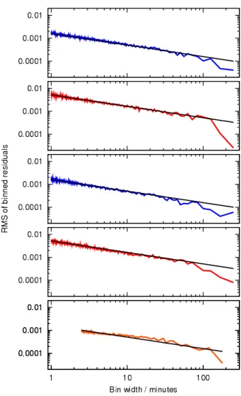
aim was to properly weight each dataset in the simultane-ous MCMC analysis and to obtain realistic uncertainties. For the five sets of WASP photometry the scale factors were in the range 0.87–0.96. The error bars of the Euler photometry were multiplied by 1.33. The scale factors for the occulta-tion photometry were in the range 1.04–1.09. Importantly, the error bars of the occultation photometry were not scaled when deciding which trend models or aperture radii to use. We assessed the presence of correlated noise in the Spitzerand Euler data by plotting the RMS of their binned residuals (Figure 7). Though there is no correlated noise ev-ident in the Spitzer data, it is present at a small level in the Euler data over time-scales of 8–80 minutes. Due to the similarity with the time-scales of the fitted features in the transit (ingress takes 36 minutes, as does egress, and the transit duration is 264 minutes), the values of some fitted parameters may be affected to a small degree.
For the same reasons as with the photometry, we added a jitter term in quadrature to the formal radial velocity er-rors, as might arise from stellar activity. We used an initial MCMC run to determine the level of jitter required for each dataset to obtain a reduced χ2 of unity. We found that the
HARPS orbital data (rv2) required a jitter of 3 m s−1 and
the HARPS spectroscopic transit data (rv4) required a jit-ter of 20 m s−1. It was not necessary to add any jitter to
either of the two CORALIE datasets.
3.6 Time systems and light travel time
The Euler photometry and the CORALIE RVs are in the BJD (UTC) time system. The WASP and Spitzer photom-etry are in the HJD (UTC) time system. The difference be-tween BJD and HJD is less than 4 s and so is negligible for our purposes. Although leap second adjustments are made
Figure 7.RMS of the binned residuals for the new Spitzer occul-tation photometry (upper four panels, with the datasets presented in the same order as in Figure 1) and the existing Euler photome-try (lower panel). The solid black lines, which are the RMS of the unbinned data scaled by the square root of the number of points in each bin, show the white-noise expectation. The ranges of bin widths (1–250 minutes for Spitzer and 2.5–180 minutes for Euler) are appropriate for the datasets’ cadences and durations.
to the UTC system to keep it close to mean solar time, mean-ing one should really use Terrestrial Time, our observations span a short baseline (2006–2008), during which there were no leap second adjustments.
The occultation of WASP-17b occurs farther away from us than its transit does, so we made a first order correction for the light travel time. We calculated the light travel time between the beginning of occultation ingress and the begin-ning of transit ingress to be 50.4 s. We subtracted this from the mid-exposure times of the Spitzer occultation photome-try. As we measure the time of mid-occultation to a precision of ±150 s, the impact of this correction was small.
4 RESULTS
Table 5 shows the median values and the 1-σ uncertainties of the fitted proposal parameters and derived parameters from our final MCMC analysis. Figure 1 shows the best-fitting
trend and occultation models together with the raw and de-trended Spitzer data. Table 2 gives the best-fitting values for the parameters of the trend models (Equation 2), to-gether with their 1 σ uncertainties. Figure 8 displays all the photometry and RVs used in the MCMC analysis, with the best-fitting eclipse and radial velocity models superimposed. From this we see that WASP-17b is a very bloated planet (Rpl = 2.0 RJup) in a slightly eccentric, 3.7 day,
ret-rograde orbit around an F6V star. By constraining the ec-centricity of WASP-17b’s orbit to low values we have shown that the circular solution presented in A10 (in which a total of three solutions were presented) is closest to reality.
4.1 Orbital eccentricity
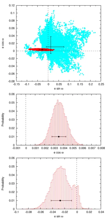
We have shown the orbit of WASP-17b to be non-circular: e cos ω is non-zero at the 4.8-σ level (e cos ω = 0.00352+0.00076
−0.00073; Figure 9), and the best-fitting solution
sug-gests that WASP-17b is occulted by its host star 12.0 ± 2.5 min later than if it were in a circular orbit. Our mea-surement of e cos ω rules out large values of e for all orbital orientations other than those with |ω| ≈ 90, and the lim-its we place on e sin ω prohiblim-its large values of e for those orientations with |ω| ≈ 90 (Figure 10). From the MCMC analysis, the 1-σ (68.3 per cent) lower and upper limits on e are, respectively, 0.010 and 0.043 and the 3-σ (99.7 per cent) lower and upper limits on e are, respectively, 0.0019 and 0.0701. We can set a more stringent 3 σ lower limit on e by assuming e sin ω ≈ 0 (and so |ω| ≈ 90), in which case it would be equal to that of the 3-σ lower limit on e cos ω: 0.0012.
Almost all values of ω are permitted by the current data, with only |ω| ≈ 90 being ruled out by the limits placed on e sin ω (Figure 10). Large values of e are consistent with the data only if |ω| ≈ 90, otherwise any orientation of the orbital major axis is permitted providing that e is small. We can thus use our measurement of e cos ω to infer a probable value of e. For random orientations of the major axis, the expected valueof cos ω is E(cos ω) = 2/π. Thus, the expected value of e is E(e) = e cos ω/ E(cos ω) = 0.0055.
We explored the effect of each occultation photometry dataset in turn on the orbital eccentricity, and of all four datasets combined. We did so by performing MCMC runs that incoporated either all, none or just one of the Spitzer datasets (Table 6; Figure 9). This demonstrates how valu-able the Spitzer occultation photometry is in determining orbital eccentricity, as its inclusion in our combined anal-ysis caused the size of the 68.3 per cent confidence val for e cos ω to decrease by a factor 30.2, and the inter-val for e sin ω to decrease in size by a factor 2.4. In addi-tion to the RV data, it is the orbital phase of the occulta-tion that constrains e cos ω and it is the occultaocculta-tion dura-tion, relative to the transit duradura-tion, that constrains e sin ω (Charbonneau et al. 2005). When including any one of the four occultation datasets, the best-fitting values of e cos ω and e sin ω obtained are consistent with the values obtained when including all four datasets. Thus no individual dataset is biasing our best-fitting solution.
Figure 9. Top panel: A comparison of the posterior probabil-ity distributions of e cos ω and e sin ω from our combined MCMC analysis when including (red dots) and excluding (cyan dots) the occultation photometry. The extent of the error bars show the 1-σ confidence limits and their intersections show the median val-ues. Middle panel: Normalised histogram of the e cos ω posterior probability distribution from our combined MCMC analysis in-coroporating the Spitzer photometry. The point with error bars, arbitrarily placed at probability = 0.01, depicts the best-fitting value and its 1-σ error bars. Bottom panel: The same plot as the middle panel, but for e sin ω.
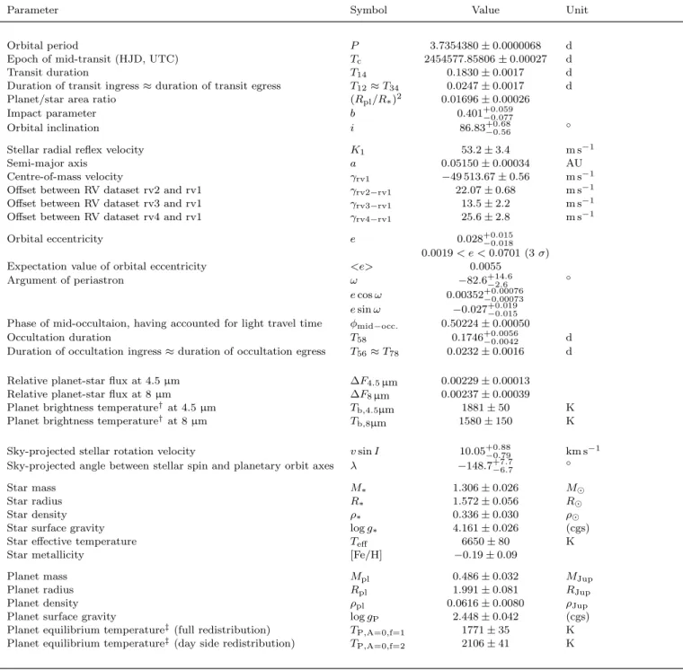
Table 5.System parameters of WASP-17
Parameter Symbol Value Unit
Orbital period P 3.7354380 ± 0.0000068 d
Epoch of mid-transit (HJD, UTC) Tc 2454577.85806 ± 0.00027 d
Transit duration T14 0.1830 ± 0.0017 d
Duration of transit ingress ≈ duration of transit egress T12≈T34 0.0247 ± 0.0017 d
Planet/star area ratio (Rpl/R∗)2 0.01696 ± 0.00026
Impact parameter b 0.401+0.059−0.077
Orbital inclination i 86.83+0.68−0.56 ◦
Stellar radial reflex velocity K1 53.2 ± 3.4 m s−1
Semi-major axis a 0.05150 ± 0.00034 AU
Centre-of-mass velocity γrv1 −49 513.67 ± 0.56 m s−1
Offset between RV dataset rv2 and rv1 γrv2−rv1 22.07 ± 0.68 m s−1
Offset between RV dataset rv3 and rv1 γrv3−rv1 13.5 ± 2.2 m s−1
Offset between RV dataset rv4 and rv1 γrv4−rv1 25.6 ± 2.8 m s−1
Orbital eccentricity e 0.028+0.015−0.018
0.0019 < e < 0.0701 (3 σ)
Expectation value of orbital eccentricity <e> 0.0055
Argument of periastron ω −82.6+14.6
−2.6 ◦
ecos ω 0.00352+0.00076−0.00073
esin ω −0.027+0.019
−0.015
Phase of mid-occultaion, having accounted for light travel time φmid−occ. 0.50224 ± 0.00050
Occultation duration T58 0.1746+0.0056−0.0042 d
Duration of occultation ingress ≈ duration of occultation egress T56≈T78 0.0232 ± 0.0016 d
Relative planet-star flux at 4.5 µm ∆F4.5µm 0.00229 ± 0.00013
Relative planet-star flux at 8 µm ∆F8µm 0.00237 ± 0.00039
Planet brightness temperature†at 4.5 µm T
b,4.5µm 1881 ± 50 K
Planet brightness temperature†at 8 µm T
b,8µm 1580 ± 150 K
Sky-projected stellar rotation velocity vsin I 10.05+0.88−0.79 km s−1
Sky-projected angle between stellar spin and planetary orbit axes λ −148.7+7.7
−6.7 ◦
Star mass M∗ 1.306 ± 0.026 M⊙
Star radius R∗ 1.572 ± 0.056 R⊙
Star density ρ∗ 0.336 ± 0.030 ρ⊙
Star surface gravity log g∗ 4.161 ± 0.026 (cgs)
Star effective temperature Teff 6650 ± 80 K
Star metallicity [Fe/H] −0.19 ± 0.09
Planet mass Mpl 0.486 ± 0.032 MJup
Planet radius Rpl 1.991 ± 0.081 RJup
Planet density ρpl 0.0616 ± 0.0080 ρJup
Planet surface gravity log gP 2.448 ± 0.042 (cgs)
Planet equilibrium temperature‡(full redistribution) T
P,A=0,f=1 1771 ± 35 K
Planet equilibrium temperature‡(day side redistribution) T
P,A=0,f=2 2106 ± 41 K
†We modelled both star and planet as black bodies and took account of only the occultation depth uncertainty, which dominates. ‡T P,A=0,f= f 1 4Teff q R∗
2a where f is the redistribution factor, with f = 1 for full redistribution and f = 2 for day side redistribution.
We assumed the planet albedo to be zero, A = 0.
5 DISCUSSION
5.1 Planet radius
With a radius of 2.0 RJup, WASP-17b is the largest known
planet by a margin of 0.2 RJup, and is over 0.7 RJuplarger
than predicted by standard cooling theory of irradiated gas giant planets (Fortney, Marley & Barnes 2007).
Ibgui & Burrows (2009) and Ibgui, Spiegel & Burrows (2011) used a coupled radius-orbit evolutionary model to
show that planet radii can be inflated to 2 RJupand beyond
during a transient phase of heating caused by tidal circular-isation of a short (a ≈ 0.1), highly eccentric (e ≈ 0.8) orbit. Though, as was noted in both studies, planets can persist in an inflated state for Gyr beyond the circularisation of their orbit and the cessation of tidal heating, they do cool and contract significantly prior to full circularisation. In each study the orbits are still significantly non-circular (e & 0.1) when the planets are largest. Thus, under the transient
heat-Figure 8. The results of our combined analysis, which combines the new Spitzer occultation photometry with existing photometry and radial velocity measurements. The models generated from the best-fitting parameter values of Table 5 are overplotted. Top-left: Occultations at 4.5 µm and, offset in relative flux by −0.01, 8 µm. The two occultations per channel from Figure 1 were binned (∆φ = 0.002, ∼11 min) together. Top-right: Transit light curve taken with Euler in the Ic-band (data from A10). Middle: Photometric
orbit and transit illustrated by WASP-South data (data from A10). Bottom: Spectroscopic orbit and transit illustrated by CORALIE and HARPS data (data from A10 and T10). The measured systemic velocities of each dataset (Table 5) have been subtracted.
Table 6.Effect of occultation light curves on best-fitting orbital eccentricity
Included occultation photometry e ω(◦) ecos ω esin ω T
occ−Tocc,circular(min)†
4.5 µm, 2009 Apr 24 0.052+0.017 −0.020 −85.9 +2.7 −1.2 0.00371 +0.00085 −0.00086 −0.051 +0.020 −0.017 12.7 ± 2.9 4.5 µm, 2009 May 1 0.0055+0.0075−0.0024 −13+82 −56 0.00302 +0.00103 −0.00098 −0.001 +0.008 −0.007 10.3 +3.5 −3.4 8 µm, 2009 Apr 24 0.015+0.059−0.012 −92 +184 −21 0.0021 +0.0039 −0.0067 −0.005 +0.011 −0.062 −7.3 +13.2 −23.2 8 µm, 2009 May 1 0.049+0.020−0.024 −82.2 +7.1 −2.4 0.00662 +0.00099 −0.00111 −0.049 +0.024 −0.020 22.7 +3.4 −3.8 None 0.038+0.045−0.026 52.6+14.6−2.6 0.011+0.027−0.018 0.013+0.062−0.021 37+92−61 All 0.028+0.015−0.018 −82.6 +14.6 −2.6 0.00352 +0.00076 −0.00073 −0.027 +0.019 −0.015 12.0 ± 2.5
All (decon. phot.) 0.022+0.016
−0.016 −81.2 +27.4 −3.7 0.00335 +0.00073 −0.00075 −0.022 +0.017 −0.016 11.5 ± 2.6 †T
occis the time of mid-occultation derived from a simultaneous MCMC analysis.
ing scenario, the very largest planets are expected to have a non-zero eccentricity. Though we do measure a non-zero ec-centricity for WASP-17b, it is small, and the stringent upper limit that we place on e is inconsistent with current models of one transient phase of tidal heating.
Other than transient heating, ongoing tidal heat-ing may occur if the orbit of a planet were kept non-circular by the continuing interaction with a third body (Ibgui, Burrows & Spiegel 2010). However, the stringent up-per limit we place on e makes this unlikely as the sole
cause of the inflation of WASP-17b, as it would necessi-tate a lower planetary tidal dissipation factor than theo-retical models or empirical determinations generally suggest (Ibgui, Burrows & Spiegel 2010).
If the atmospheric opacity of WASP-17b were enhanced then its internal heat would be lost at a lower rate and con-traction would be slowed (Burrows et al. 2007). The atmo-spheric opacities of WASP-17b may be enchaned if, for ex-ample, the strong optical and UV irradiation of the planet by
Figure 10. The range of e and ω permitted by the available data. The black dot with error bars shows the best-fitting values from our combined MCMC analysis. The grey dots are the values in accepted MCMC steps. The solid blue and red lines show the values of e and ω that would be indicated by, respectively, the best-fitting values of e cos ω and e sin ω on their own. The dashed and the dotted lines bound the parameter space permitted by the 1-σ and the 2-σ limits, respectively, on those parameters, with the same colour scheme applying. Note that, as the 2-σ upper limit on e sin ω is positive, almost all values of ω are consistent with the data at the 2-σ level (providing e < 0.01).
its host star produces thick hazes, absorbing clouds and non-equilibrium chemical species (e.g. tholins or polyacetylenes). The bloated planets are all very strongly irradiated by their host stars, and a small fraction of stellar insolation en-ergy would be sufficient to account for the observed degrees of bloating. Guillot & Showman (2002) suggested that the kinetic energy of strong winds, induced in the atmosphere of a short-period planet by the large day-night temperature contrasts that result from tidal locking, may be transported downward and deposited as thermal energy in the deep in-terior. However, a mechanism to convert the kinetic energy into thermal energy would still be required. Li & Goodman (2010) and Youdin & Mitchell (2010) found that turbulence is efficient at dissipating kinetic energy. Magnetic drag on weakly ionized winds (Perna, Menou & Rauscher 2010) and Ohmic heating (Batygin & Stevenson 2010) are alternative mechanisms.
5.2 Planetary atmosphere
Fortney et al. (2008) hypothesise that the presence of high opacity TiO and VO gases in the atmospheres of highly irra-diated planets (those experiencing an incident flux of > 109
erg s−1 cm−2) cause them to have temperature inversions.
Thus, with an incident flux of 2.2 ± 0.2 × 10⁹ erg s−1cm−2,
WASP-17b is expected to have an atmospheric temperature inversion under this hypothesis.
However, Spiegel, Silverio & Burrows (2009) suggest that, for a planet with the insolation level of WASP-17b, it is unlikely that a temperature inversion could be caused by the presence of TiO and VO in the upper atmosphere. They find that a cold trap exists between the hot convection zone and the hot upper atmosphere on the irradiated day
side, in which titanium is likely to form condensates that settle more strongly than does gasesous TiO. Therefore, un-less there is extremely vigorous macroscopic mixing and the condensed Ti is lofted back in to the upper atmosphere then it is unlikely that TiO can explain the observed temperature inversions. Not only does VO have the same ‘cold trap’ is-sue, but it also has a lower opacity than TiO and is an order of magnitude less abundant.
Knutson, Howard & Isaacson (2010) suggest that plan-ets orbiting chromospherically active stars do not have tem-perature inversions, and planets orbiting quieter stars do have inversions. They suggest that the high UV flux that planets orbiting active stars are likely to experience de-stroys the compounds responsible for the observed temper-ature inversions. Knutson, Howard & Isaacson (2010) find the two classes to be delineated by a host-star activity level of log(R′HK) ≈ −4.9. Though they caution that the
calibra-tion for log(R′HK) is uncertain for stars as hot as WASP-17,
they measure the star to be quiet: log(R′HK) = −5.3.
WASP-17b is therefore expected to have an atmospheric tempera-ture inversion under this hypothesis as well.
In Figure 11, the measured 4.5 and 8 µm planet-star flux-density ratios are compared to two model atmosphere spectra of the planet (Barman, Hauschildt & Allard 2005), with parameters taken from Table 5. A black-body (TP,A=0=
1600 K) is a poor fit to the data and is thus ruled out. In one model atmosphere TiO produces a temperature inversion across the photospheric depths. In the other model, there is no atmospheric TiO. The two models have near-identical 4.5 and 8 µm absolute fluxes, and so we can not currently discriminate between the two. A precise measurement at 3.6 µm may distinguish between the two cases and thus reveal whether WASP-17b has an atmospheric temperature inver-sion.
By modelling the planet and star as black bodies, we used the measured planet-star flux-density ratios to calcu-late 4.5 and 8 µm brightness temperatures of 1881 ± 50 K and 1580 ± 150 K, respectively. We calculate an equilibrium temperature TP,A=0,f=1 = 1771 ± 35 K by modelling the
planet as a black body with efficient redistribution of en-ergy from its day side to its night side. The closeness of the brightness temperatures to this equilibrium temperature is consistent with the planet having a low albedo and efficient heat redistribution.
5.3 Misaligned orbit
WASP-17b is in a retrograde orbit. For planet-planet or star-planet scattering to have caused the misalignment between the orbit of WASP-17b and the spin axis of its host star, an additional body must have been present. We looked for evidence of a long-term drift ˙γ in the radial velocity mea-surements, which span 716 days, as may be caused by the presence of a long-period companion. From a straight-line fit to the residuals of the radial velocities about the best-fitting model, we get ˙γ = −6 ± 5 m s−1 yr−1. Hence, there
is currently no evidence for a third body in the system, but this does not preclude planet-planet scattering as the cause of the misalignment. Nagasawa, Ida & Bessho (2008) found, whilst showing that a combination of planet-planet scatter-ing and the Kozai mechanism can put planets into short,
Figure 11.Comparison of planet-star flux density measurements with two model planet atmospheres and with a black-body. The model atmosphere with TiO exhibits a temperature inversion that extends down to photospheric depths, whilst the model without TiO does not. Inset: Temperature-pressure profiles for the two model atmospheres.
retrograde orbits, that the outer planets can end up at large orbital distances, making them difficult to detect, or they can be ejected from the system.
5.4 System age
We interpolated the stellar evolution tracks of Marigo et al. (2008) using ρ∗ from Table 5 and the values of Teff and
[Fe/H] from T10 (Figure 12). This suggests an age of 2.65 ± 0.25 Gyr and a mass of 1.20 ± 0.05 M⊙for WASP-17.
Assuming the stellar-spin axis to be in the sky plane, the measured v sin I of WASP-17 and its derived stellar radius (Table 5) indicate an upper limit to the rotational period of Prot = 7.91 ± 0.75 d. Combining this with the B − V
colour of an F6V star from Gray (2008), and the relation-ship of Barnes (2007), we estimate an upper limit on the gyrochronological age of 1.9 ± 0.5 Gyr. We found no evi-dence for rotational modulation in the WASP light curves.
We calculated a tidal circularisation time-scale of τcirc=
5 Myr for WASP-17b by using the best-fitting values of the planetary (QP = 105.5) and stellar (Q∗ = 106.5) tidal
dis-sipation factors of Jackson, Greenberg & Barnes (2008a) in their Equation 1. As the values of the tidal dissipation fac-tor are highly uncertain (QP= 105–108, Q∗= 105–108, e.g.
Ibgui, Spiegel & Burrows 2011), a range of τcirc = 2–1700
Myr is possible.
With Teff = 6650 ± 80 K (T10), WASP-17 is in the
‘Lithium gap’ (or ‘dip’), which is the range of Teff = 6600 ±
150 K in which stars are depleted in lithium by a factor of 30 or more than in hotter and cooler stars (see Balachandran 1995, and references therein). The upper limit placed on the
Figure 12.Modified H-R diagram. The isochrones (Z = 0.012 ≈ [Fe/H] = −0.19) for the ages 0.5, 1, 2, 2.5, 3, 4, and 5 Gyr are from Marigo et al. (2008) and the evolutionary mass tracks (Z = 0.012 ≈ [Fe/H] = −0.019; Y = 0.30) are from Bertelli et al. (2008). To obtain the mass tracks, we performed a simple linear interpolation of their Z = 0.0008 and Z = 0.017 tracks.
lithium abundance (ALi < 1.3) in A10 is consistent with
this. Thus, lithium is not an effective indicator of age for WASP-17.
6 CONCLUSIONS 6.1 Science
With a radius of 2.0 RJup, WASP-17b is larger than any
other known planet by 0.2 RJup and it is 0.7 RJup larger
than predicted by standard cooling theory of irradiated gas giant planets. The extent of the planet’s inflation is difficult to explain with current models.
Our Spitzer occultation photometry gives much tighter constraints on orbital eccentricity than existing radial veloc-ity data alone, thus permitting an accurate determination of the stellar and planetary radii. We have shown that WASP-17b is in a slightly eccentric orbit, with 0.0017 < e < 0.0701. The stringent upper limit we have placed on eccentricity sug-gests that a transient phase of tidal heating alone could not have inflated the planet to its measured radius. Nor could ongoing tidal heating involving a third body, unless the plan-etary tidal quality factor is smaller than the best theoretical and empirical determinations.
We find no evidence in the radial velocity measurements for a third body in the system, the presence of which would be necessary to excite the eccentricity of WASP-17b for tidal heating to be ongoing, and may have been necessary to mis-align the planet’s orbital axis with the spin axis of the star. Our 4.5 and 8 µm planet-star flux-density ratios do not probe the existence of the expected atmospheric tempera-ture inversion, but a measurement at 3.6 µm may do so. Though the ratios are inconsistent with a black-body atmo-sphere, they are consistent with a low-albedo planet that efficiently redistributes heat from its day side to its night side.
6.2 Spitzer data
To determine correctly the photometric uncertainties and the optimal aperture radii to use for Spitzer data, account must be taken of the counts removed during sky-dark sub-traction.
When the background is bright relative to the target at 8 µm, the measured occultation depth can depend sen-sitively on the choice of aperture radius. In these circum-stances detrending with detector position vastly reduces the dependency. An alternative is to perform deconvolution pho-tometry.
In addition to the known hour-long oscillations of Spitzer’s pointing about the nominal position, there is also a high-frequency jitter, with periods of 1–2 minutes. So, when accounting for the inhomogeneous detector response (or ‘pixel phase’ effect), one should detrend target flux with the unsmoothed target detector positions.
ACKNOWLEDGMENTS
This work is based in part on observations made with the Spitzer Space Telescope, which is operated by the Jet Propulsion Laboratory, California Institute of Technology under a contract with NASA. Support for this work was pro-vided by NASA through an award issued by JPL/Caltech. M. Gillon acknowledges support from the Belgian Science Policy Office in the form of a Return Grant.
REFERENCES
Anderson D. R. et al., 2010a, A&A, 513, L3+ —, 2010b, ApJ, 709, 159
Balachandran S., 1995, ApJ, 446, 203 Barman T. S., 2008, ApJ, 676, L61
Barman T. S., Hauschildt P. H., Allard F., 2005, ApJ, 632, 1132
Barnes S. A., 2007, ApJ, 669, 1167
Batygin K., Stevenson D. J., 2010, ApJ, 714, L238 Bayliss D. D. R., Winn J. N., Mardling R. A., Sackett P. D.,
2010, ApJ, 722, L224
Bertelli G., Girardi L., Marigo P., Nasi E., 2008, A&A, 484, 815
Burrows A., Hubeny I., Budaj J., Hubbard W. B., 2007, ApJ, 661, 502
Charbonneau D. et al., 2005, ApJ, 626, 523
Charbonneau D., Knutson H. A., Barman T., Allen L. E., Mayor M., Megeath S. T., Queloz D., Udry S., 2008, ApJ, 686, 1341
Collier Cameron A. et al., 2007, MNRAS, 380, 1230 Enoch B., Collier Cameron A., Parley N. R., Hebb L., 2010,
A&A, 516, A33+
Fabrycky D., Tremaine S., 2007, ApJ, 669, 1298 Fazio G. G. et al., 2004, ApJS, 154, 10
Ford E. B., 2006, ApJ, 642, 505
Ford E. B., Rasio F. A., 2008, ApJ, 686, 621
Fortney J. J., Lodders K., Marley M. S., Freedman R. S., 2008, ApJ, 678, 1419
Fortney J. J., Marley M. S., Barnes J. W., 2007, ApJ, 659, 1661
Fressin F., Knutson H. A., Charbonneau D., O’Donovan F. T., Burrows A., Deming D., Mandushev G., Spiegel D., 2010, ApJ, 711, 374
Gaudi B. S., Winn J. N., 2007, ApJ, 655, 550
Gillon M., Magain P., Chantry V., Letawe G., Sohy S., Courbin F., Pont F., Moutou C., 2007, in Astronomical Society of the Pacific Conference Series, Vol. 366, Tran-siting Extrapolar Planets Workshop, C. Afonso, D. Wel-drake, & T. Henning, ed., pp. 113–+
Gillon M., Pont F., Moutou C., Bouchy F., Courbin F., Sohy S., Magain P., 2006, A&A, 459, 249
Gray D. F., 2008, The Observation and Analysis of Stellar Photospheres, Gray, D. F., ed.
Guillot T., Showman A. P., 2002, A&A, 385, 156
Harrington J., Luszcz S., Seager S., Deming D., Richardson L. J., 2007, Nature, 447, 691
Howell S. B., 1989, PASP, 101, 616 Ibgui L., Burrows A., 2009, ApJ, 700, 1921
Ibgui L., Burrows A., Spiegel D. S., 2010, ApJ, 713, 751 Ibgui L., Spiegel D. S., Burrows A., 2011, ApJ, 727, 75 Jackson B., Greenberg R., Barnes R., 2008a, ApJ, 678, 1396 —, 2008b, ApJ, 681, 1631
Knutson H. A., Charbonneau D., Allen L. E., Burrows A., Megeath S. T., 2008, ApJ, 673, 526
Knutson H. A., Howard A. W., Isaacson H., 2010, ApJ, 720, 1569
Leconte J., Chabrier G., Baraffe I., Levrard B., 2010, A&A, 516, A64+
Li J., Goodman J., 2010, ApJ, 725, 1146
Magain P., Courbin F., Gillon M., Sohy S., Letawe G., Chantry V., Letawe Y., 2007, A&A, 461, 373
Magain P., Courbin F., Sohy S., 1998, ApJ, 494, 472 Marigo P., Girardi L., Bressan A., Groenewegen M. A. T.,
Silva L., Granato G. L., 2008, A&A, 482, 883 Nagasawa M., Ida S., Bessho T., 2008, ApJ, 678, 498 Perna R., Menou K., Rauscher E., 2010, ApJ, 719, 1421 Pollacco D. et al., 2008, MNRAS, 385, 1576
Press W., Flannery B., Teukolsky S., Vetterling W., 1992, Numerical Recipes in C: The Art of Scientific Computing. Cambridge University Press
Reach W. T. et al., 2005, PASP, 117, 978
Schwarz G., 1978, The Annals of Statistics, 6, 461 Seager S., Mall´en-Ornelas G., 2003, ApJ, 585, 1038 Shannon C., 1949, Proceedings of the IRE, 37, 10
Spiegel D. S., Silverio K., Burrows A., 2009, ApJ, 699, 1487 Swain M. R., Vasisht G., Tinetti G., Bouwman J., Chen P., Yung Y., Deming D., Deroo P., 2009, ApJ, 690, L114 Triaud A. H. M. J. et al., 2010, A&A, 524, A25+
Werner M. W. et al., 2004, ApJS, 154, 1
Wheatley P. J. et al., 2010, ArXiv e-prints arXiv:1004.0836 Youdin A. N., Mitchell J. L., 2010, ApJ, 721, 1113