Credit risk structural models with finite grace delays

UNIVERSITÉ DU QUÉBEC À MONTRÉAL

CREDIT RISK STRUCTURAL MODELS WITH FINITE GRACE DELAYS

A THESIS PRESENTED

AS PARTIAL REQUIREMENT

OF THE DEGREE OF MASTER'S IN MATHEMATICS

BY

ADEL BENLAGRA

UNIVERSITÉ DU QUÉBEC À MONTRÉAL

MODÈLES STRUCTURELS EN RISQUE DE CRÉDIT AVEC DÉLAIS DE GRÂCE

MÉMOIRE PRÉSENTÉ

COMME EXIGENCE PARTIELLE DE LA MAÎTRISE EN MATHÉMATIQUES

PAR

ADEL BENLAGRA

UNIVERSITÉ DU QUÉBEC À MONTRÉAL Service des bibliothèques

Avertissement

La diffusion de ce mémoire se fait dans le respect des droits de son auteur, qui a signé le formulaire Autorisation de reproduire et de diffuser un travail de recherche de cycles supérieurs (SDU-522 - Rév.1 0-2015). Cette autorisation stipule que «conformément à · · l'article 11 du Règlement no 8 des études de cycles supérieurs, [l'auteur] concède à l'Université du Québec à Montréal une licence non exclusive d'utilisation et de publication de la totalité ou d'une partie importante de [son] travail de recherche pour des fins pédagogiques et non commerciales. Plus précisément, [l'auteur] autorise l'Université du Québec à Montréal à reproduire, diffuser, prêter, distribuer ou vendre des copies de [son] travail de recherche à des fins non commerciales sur quelque support que ce soit, y compris l'Internet. Cette licence et cette autorisation n'entraînent pas une renonciation de [la] part [de l'auteur] à [ses] droits moraux ni à [ses] droits de propriété intellectuelle. Sauf entente contraire, [l'auteur] conserve la liberté de diffuser et de commercialiser ou non ce travail dont [il] possède un exemplaire.»

REMERCIEMENTS

Je remercie tous ceux qui, de près ou de loin, m'ont soutenu dans mes décisions, au cours des mes études et qui ont contribué, chacun à sa manière, à la réussite de ce projet.

Merci aux professeurs Jean-François Renaud et Mathieu Boudreault qui m'ont dirigé lors de ce mémoire et bien plus. Le professeur Renaud m'a donné sa co nfi-ance, en sa qualité de directeur des programmes de cycles supérieurs, pour revenir sur les bancs de l'université en veillant soigneusement à comprendre ma démarche et en me conseillant pour la faire aboutir au mieux. Le professeur Boudreault a été présent tout au long de ma maitrise par l'effervescence de ses idées et son é n-ergie qui forcent l'admiration. Il s'est toujours assuré que ma maitrise se déroule dans les meilleures conditions possibles et cela a été le cas en grande partie grâce à lui.

Ma gratitude va pour mon épouse qui a sacrifié bien plus que moi, tout au long de ma maitrise et de mon mémoire, en me libérant de toute autre responsabilité que celle d'étudier et d'enseigner. Sans son support, peut être aurais-je manqué de courage ou de détermination.

Mon amitié est quant à elle pour mon collègue de bureau Amine Mohamed Lk-abous avec qui j'ai partagé de gros moments de bonne humeur et d'intenses dis -cussions qui m'ont éclairé à bien des égards.

LISTE DES FIGURES 0 RÉSUMÉ 0 0 0 0 0 INTRODUCTION

CONTENTS

CHAPTER I STRUCTURAL MODELS IN CREDIT RISK 1.1 Basic assumptions and notations

1.2 Merton's model 0 0 0 0 0 0 1.3 First-passage-time models

10 3 01 First-passage times and their properties 1.302 Black and Cox model 0 0 0

1.303 Optimal capital structure

1.304 Extensions of the Black and Cox model 0

CHAPTER II STOPPING TIMES FOR THE MODELLING OF GRACE Vll xi 1 7 7 8 10 10 11 12 13 DELAYS 0 0 0 0 0 0 0 0 0 0 0 0 0 0 0 0 0 0 0 0 0 0 0 0 0 0 0 0 0 0 17 201 A generalized state variable and its associated default time 17

202 The excursive (Parisian) case 0 20

203 The cumulative (Parasian) case

20301 The joint distribution of ( Zt, A~'z) 2.4 Summary of the main analytical results 0

22 22 24

205 A Monte Carlo study of default times 0 0 26

CHAPTER III A MODEL WITH A GRACE DELAY AND FINITE

MA-TURITY 0 0 0 0 0 0 0 0 0 0 0 0 0 0 0 0 33

301 The model and capital structure 0 0 33

301.1 The corporate coupon bond 301.2 The optimal capital structure

33 34

Vl

3.2 The perpetual debt case (T --+ +oo) 3.2.1 The endogenous barrier 3.2.2 The optimal delay 3.3 The finite maturity case .

3.3.1 The limit of no grace delay ( d--+ 0) 3.3.2 The case of a finite grace delay . . CHAPTER IV A MODEL OF 11

ROLL-OVER11

DEBT WITH A GRACE 35 37 38 39 39 40 DELAY . . . . . . . . . . . . . . . . . 45

4.1 The model and capital structure . . 45

4.1.1 The roll-over debt structure 4.1.2 The corporate coupon bond 4.1.3 The optünal capital structure 4.2 Main results . . . . . . . . . .

4.2.1 The debt, firm and equity values 4.2.2 The endogenous barrier

4.2.3 The optimal delay CONCLUSION

APPENDIX A USEFUL INTEGRALS AND MATHEMATICAL PROP-45 46 47 48 48 50 55 57 ERTIES . . . 59 A.1 Integrals . . . . . . . . . . . . . . . . 59 A.2 Derivatives of the bivariate normal di tribution function 60

APPENDIX B THE DISTRIBUTION FUNCTION OF A~z . 61

APPENDIX C DETAILS OF THE ANALYTICAL CALCULATION OF

IE [ E-rt1o ]_{Oo:ST}] 65

LISTE DES FIGURES

Figure Page

1.1 Default times in Merton and Black-Cox models. . . 11 2.1 Evolution of the process (left) and the state variable

I

f

(right)

with time in the Parisian and Parasian cases. The chosen default time is such that the state variable is bigger than d = 4. We used r = 7.5%, q = 7%, CJ = 20%, K = 0.950 . . . . 18 2.2 Survival probability in the cumulative and excursive cases when

the maturity is infinite and the Q-trend is positive. We used r = 6%, q = 1%, CJ = 30%, K = 0.950, F = 0.9550 . The dotted line is a visual guide for a survival probability equal to O. 7 and the corresponding grace delays to achieve it in the excursive and cumulative cases. . . . . . . . . . . . . . . . . . 25 2.3 The ratio defined in equation (2.35) for n

=

0 (left) and n

=

1

(right). We used r

=

6%, CJ

=

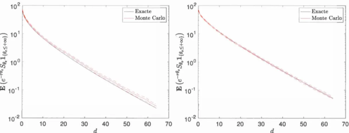
29%. . . . . . . . . . . . . . 26 2.4 Comparison between the exact expression of (2.8) and its estima

-tion by a naive MC algorithm in the Parisian (left) and Parasian (right) cases. We used r = 7.5%, q = 7%, CJ = 20%, K = 0.950, n = 1, T = 1000, h = 0.1 and a Monte Carlo sample of size N = 1000. The dashed lin es show the 95% confidence interval for the Monte Carlo estimation. . . . . . . . . . . . . . . . . . . . 28 2.5 Evolution of the state variable

If

in time for various values of the

parameters

/3,

r

and functional form off. We used r

=

6%, q

=

1%,CJ = 29%,K = 0.95S₀,h = 0.1 and a Monte Carlo sample of size N = 10000. . . . . . . . . . . . . . . . . . . 29 2.6 Correlation between the default times of cases 2-5 and the default

time of case 1. We used r = 6%, q

=

1%, CJ

=

29%, K = 0.9550 , h = 0.1 and a Monte Carlo sample of size N

=

10000. . . . . . . . 30

Vlll

2. 7 Comparison of the standard errors obtained in the naive and the control variate MC for cases 3 (left) and 4 (right). We used r = 6%, q = 1%, 0' = 29%, K = 0.95S0, h = 0.1 and a Monte Carlo

sample of size N

=

10000. 30

3.1 Debt (left) and equity (right) values as functions of the grace delay d for different values of the coupon rate c. We used r = 6%, q = 1%, 0' = 30%, I< = 0.9S0, F = 0.95S0, a0 = 40%, n =O. . 36 3.2 Debt (left) and equity (right) values as functions of the grace delay

d for different values of the barrier K. We used r = 6%, q = 1%, c = 4%, 0' = 30%, F = 0.95, S₀, a₀ = 40%, n = O. 36 3.3 Minünum between the endogenous barrier K* and S₀ as function of

the grace delay d. We used r = 6%, q = 1%, c = 4%, 0' = 30%, F =

0.95, S0, a0 = 40%, n =O. . 38

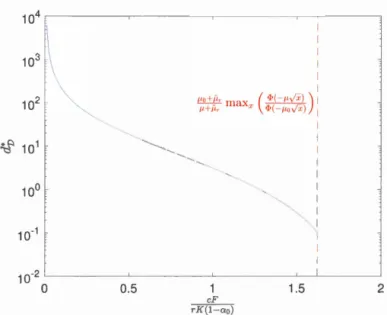
3.4 The optimal delay

d1J

minimizing the debt value in the perpetua! case as a function of rK(~~an) with n = O. We used r = 6%, q =

1%, 0' = 30%. 40

3.5 Debt (left) and equity (right) values as functions of the grace delay d for different values of the coupon rate c. We used r

=

6%, q

=

1%, 0' = 30%, Ç = 0%, K = 0.9S0 , F = 0.8S0, R = 0.6, n = O. . 41 3.6 Minimum between the endogenous barrier K]J and S0 as a function

of th grac delay d with n

=

0 and different values of T. We used r = 6%, q = 1%, 0' = 30%, a = 40%, c = 0.6r. 41 3.7 The optimal delay

dv

minimizing the debt value for a finite m

a-turity T

=

30 as a function of rK(~~ao) with n

=

0 and different values of a0 . We used r = 6%, q = 1%, 0' = 30%. 42 3.8 The optimal delay

d1J

minimizing the debt value for a finite m

a-turity T

=

30 as a function of rK(~~ao) with n

=

0 and different values of a0 . We used r = 6%, q = 1%, 0' = 30%. 43 4.1 The debt (top left), equity (top right) and firm (bottom) values as

functions of the grace delay length d and the n1ean mat uri ty Tm in the cumulative case. We used r = 6%, q = 1%, 0' = 30%, P = 95, c = 2.4%, K = 90,17 = 1, n = O. . 50

4.2 The equity value as a function of the barrier K for two different values of the delay d.

Ki

and

K

;P

are shown by, respectively, a black and a red dashed line. We used r = 6%, q = 1%, a = 30%, P =

ix

95, c = 2.4%, Sa= 100, 'Tl= 1, n =O. . . . . . . . . . . . . . . . . . 52 4.3 The endogenous barrier obtained from maximizing the equity (left)

and from the smooth pasting condition of (4.23) (right) as a func-tion of the grace delay length d and the mean maturity Tm in the cumulative case. We used r = 6%,q = 1%,a = 30%, P = 95,c = 2.4%,SO = 100,ry = 1,n =O. . . . . . . . . . . . . . . . . . . . . . 52 4.4 The equity value as function of Sa for values larger than Kt:*. We

used r = 6%, q = 1%, a = 30%, P = 95, c = 2.4%, SO = 100, 'Tl = 1,n = O,m = 0.1,d = 5. . . . . . . . . . . . . . . . . . 53 4.5 The endogenous barriers obtained from maximizing the equity in

the excursion and cumulative cases as functions of the grace delay length d and the mean maturity Tm· We used r = 6%, q = 1%, a= 30%, P = 95, c = 2.4%, SO = 100, K = 90, 'Tl= 1, n =O. . . . . . . 54 4.6 The endogenous barrier obtained from minimizing the debt value

as a function of the grace delay length d and the mean maturity Tm

in the cumulative case. We used r = 6%, q = 1%, a = 30%, P = 95, c = 2.4%,SO = 100,ry = 1,n =O.. . . . . . . . . . . . . . . . . 55 4. 7 The optimal delay

dv

that minimizes the debt as a function of the

mean maturity Tm and the coupon rate c. We used r = 6%, q = 1%, a= 30%, P = 95, c = 2.4%, K = 90, 'Tl= 1, n =O. . . . . . . . 56

RÉSUMÉ

Ce mémoire porte sur une extension des 1nodèles structurels en risque de crédit basés sur le concept de temps de premier passage. Dans ces modèles-là, le défaut est généralement déclaré dès que la valeur des actifs d'une compagnie baisse en dessous d'un niveau donné. La généralisation considérée ici consiste à accorder un délai de grâce pour permettre à la compagnie de se reprendre avant que le défaut ne soit éventuellement déclaré.

En nous basant sur des résultats théoriques développés dans d'autres contextes, comme la théorie des options parisiennes ou celle des temps d'occupation en théorie de la ruine, nous arrivons à dériver des formules analytiques exactes pour les valeurs marchandes de la dette ainsi que des actifs de la compagnie et ce pour plusieurs modèles de dette corporative. Nos résultats permettent, entre autres, d'analyser l'effet de ce délai sur la barrière endogène qui optimise la structure du capital de la compagnie ou d'optimiser le délai de grâce accordé afin de minimiser la dette ou de maximiser le valeur des actifs. Nos formules exactes pourraient également être mises à profit dans la technique de la variable de contrôle afin de minimiser la variance des estimateurs de Monte Carlo pour des cas où il n'y a aucune formule analytique connue.

Mots clés: Risque de défaut, processus de diffusion, modèles structurels, délai de grâce, options parisiennes, structure optimale de capital.

ABSTRACT

This thesis focuses on an extension of the structural models in credit risk which are based on the concept of first-passage times. In these models, default is usually declared as soon as the value of a company's assets drops below a given level. The generalization presented here considers a finite grace period given to the company, once its assets' value drops below a given barrier, to recover before default is eventually declared.

Based on theoretical results developed in other contexts, such as the theory of Parisian options or the time of occupation in ruin theory, we derive exact analytical formulas for the market values of debt as well as the assets value of the company and this for several models of corporate debt. Our results make it possible, among other things, to analyze the effect of this delay on the endogenous barrier that optimizes the capital structure of the company or to optimize the grace period granted in order to minimize the debt or maximize the value of the assets .. Our exact formulas could also be used in the control variable technique to minimize the variance of Monte Carlo estimators for cases where there is no known analytical formula.

Keywords: Default risk, diffusion process, structural models, grace period, Parisian options, optimal capital structure.

INTRODUCTION

La présente introduction décrit brièvement les modèles classiques de l'approche structurelle au risque de crédit afin de situer la portée de nos travaux et leur contribution à la littérature.

L'approche structurelle relie le défaut d'une firme à la dynamique sous-jacente de ses actifs représentée par un processus de diffusion St. Une classe importante des modèles structurels est celle basée sur les temps de premier passage où le défaut et/ ou la liquidation sont déclarés dès que la valeur des actifs de la firme descend en dessous d'une certaine barrière Kt. Cette dernière peut être déterminée de façon exogène ou endogène afin d'optimiser la structure du capital. Le premier cas a été étudié, par exemple, par Black et Cox (Black & Cox, 1976). La barrière endogène a été considérée par Leland (Leland, 1994b) et Leland et Toft (Leland

& Toft, 1996) et est définie comme la barrière qui maximise la valeur de l'équité

(et minimise dans leur cas la valeur de la dette). Dans le cadre de ce dernier modèle, une dette à structure "roll-over" retirée et ré-émise à un taux m avec un profil de maturité de distribution exponentielle est considérée. Ce modèle de dette est riche et flexible et permet d'obtenir des formules analytiques fermées, en particulier dans les limites m

---+

0, +oo.

Dans les études sus-citées, l'actif suit un processus de diffusion à volatilité con-stante, le plus souvent le modèle de Black et Scholes. Une des faiblesses d'un modèle à diffusion dans le cadre structurel est que les écarts de crédit (credit spread), en particulier pour les courtes maturités, ne correspondent pas aux don-nées empiriques. Notamment, les écarts de crédit à très court terme sont nuls. Ceci est relié au fait que l'entreprise ne peut pas faire défaut sur une courte péri-ode par surprise parce qu'il ne peut y avoir de diminution soudaine de la valeur de l'actif. D'où la nécessité, par exemple, de considérer la présence de sauts dans l'évolution de l'actif.

Zhou (Zhou, 1997) a été l'un des premiers à utiliser un modèle de diffusion avec sauts. Dans ce modèle, l'intensité des sauts suit une loi log-normale. La présence de ces derniers produit une structure à terme des écarts de crédits plus riche (forme croissante, plate, hump-shaped, ... etc) qui n'existe pas quand le processus

2

est purement diffusif. De plus, comme attendu, l'écart de crédit à courte maturité est non nul.

D'autres types de modèles à sauts ont été considérés comme celui du modèle basé sur les processus de Lévy spectralement négatifs (SNLP), dans le cadre de l'approche de Leland et Toft, par Hilberink et Rogers (Hilberink & Rogers, 2002) ou le modèle à double exponentielle de Kou (Kou, 2002) par Chen et Kou (Chen

& Kou, 2009). Ces derniers reprennent le modèle de dette "roll-over" de Leland et, en dérivant des formules analytiques semi-fermées, font une étude exhaustive de la structure du capital, des écarts de crédits et la fonne de leur structure à terme, de la volatilité implicite associée à la valeur de l'équité et de la barrière endogène de défaut. Dao et Jeanblanc (Dao & Jeanblanc, 2006) ainsi que Le Courtois et Quittard-Pinon (Le Courtois & Quittard-Pinon, 2006) calculent également la barrière endogène de défaut et étudient la probabilité de liquidation.

Tous les 1nodèles 1nentionnés ci-dessus se situent uniquement dans le cadre des modèles de temps de premier passage. En effet, ils considèrent que le signal de détresse financière, que représente la diminution de la valeur des actifs en dessous de la barrière, doit impérativement être accompagné par un défaut immédiat. On pourrait néanmoins considérer la possibilité d'accorder à la firme un délai de grâce

d entre le moment où elle entre en détresse financière, tel que défini plus haut, et le moment où son défaut est déclaré. En effet, le signal de détresse pourrait être ponctuel dans le temps. Aussi, la compagnie pourrait se redresser au bout d'un certain temps auquel cas il n'y a pas lieu de déclarer sa faillite tout de suit .

Des 1nécanismes, co1nme le chapitre 11 de la loi sur les faillites des États-Unis, permettent justement de telles possibilités. Il serait alors opportun d'analyser

l'effet d'un délai de grâce afin de séparer le moment de défaut formel du signal de détresse.

De récentes études vont dans ce sens, en considérant souvent le modèle de Black et Scholes ou des cas simples de maturité infinie afin de simplifier les calculs.

François et Morellec (François & Morellec, 2004) considèrent le cas où la liquida

-tion est déclarée si le temps passé par 1 'actif de la firme sous la barrière de détresse dépasse, continûment, une période de grâce d. C'est un modèle basé sur le temps

d'excursion: si

g

J:'

5 est le dernier temps où la détresse financière est signalée pour un te1nps t (voir la définition formelle à l'équation (1.18)), le temps d'excursion est

t-

g

J:'

5. La dette considérée étant perpétuelle, et la dynamique sous-jacente étant celle de Black et Scholes, ils obtiennent des formules analytiques pour la valeur de

3

la firme, de l'équité et de la dette en se basant sur les résultats de Chesney et al. (Chesney et al., 1997) pour les options parisiennes. Ils obtiennent également la

formule de la barrière endogène en maximisant la valeur de l'équité en fonction de la barrière. Broadie et al. (Broadie et al., 2007) étendent l'étude à des maturités

finies en résolvant numérique1nent des équations aux dérivées partielles pour le calcul de la valeur de la dette et de l'équité.

Moraux (Moraux, 2002) considère un modèle basé sur le temps d'occupation

A

{<,s

=

J~ ]_{Su:'SKu}du, c'est à dire le temps passé cumulativement sous la ba r-rière. Le défaut est formellement déclaré au temps

e

= inf { u ~ OIA~,s ~ d}. En utilisant des résultats de Hugonnier (Hugonnier, 1999) sur les options utilisant les

temps d'occupation du mouvement brownien, Moreaux trouve des formules ana

-lytiques semi-fermées, basées sur des transformées de Laplace, pour la valeur de la dette et de l'équité dans le cas d'une maturité finie. Makarov et al. (Makarov

et al., 2015) utilisent les mêmes résultats pour calculer d'autres quantités comme la probabilité de liquidation, la valeur espérée de la perte étant donnée la

liquida-tion, etc. Ces résultats semi-analytiques requièrent le calcul de doubles intégrales et ne permettent pas d'avoir une compréhension du modèle sans le calcul de ces intégrales. Notamment, il est ardu d'analyser certaines limites comme d ---+ 0 ou

une maturité T ---+ +oo.

Galai et al. (Galai et al., 2007) considèrent des temps d'occupation généralisés

de la forme

K,S t

ItK,S = [9t e-f3(t-u) f(Su)du

+

{K s e-"((t-u) f(Su)du,

h

~t' (1)

qui permettent de prendre en compte les précédentes périodes sous la barrière de

défaut ainsi que leur sévérité (l'interprétation de ces temps d'occupation génér al-isés sera abordée plus en détail au chapitre 2).

Le défaut est déclaré lorsque

e

= inf { u ~ OIJ~<,S ~ d} est inférieur à la ma tu-rité

T

de la dette. La variable

I

{<,s

se réduit au temps d'excursion ou au temps

d'occupation selon les valeurs de

/3,1

et la forme fonctionnelle de f. Elle pe r-met de prendre en compte la sévérité du défaut pour un choix approprié de la

fonction

f

ainsi que la contribution des précédentes périodes de détresse dans la comptabilisation du temps passé sous la barrière. Galai et al. étudient ensuite,

numériquement en résolvant une équation aux dérivées partielles et en l'absence

de formules analytiques dans le cas général, la valeur de la dette et de l'équité et l'écart de crédit pour plusieurs valeurs de (3, ry et choix de la fonction f. La

4

Chang et al. (Chang & Lee, 2013) utilisent une simulation Monte Carlo basée sur

le pont brownien ( Brownian bridge) pour étudier la probabilité de défaut et les écarts de crédit dans le modèle de Kou. Bruche et al. (Bruche & Naqvi, 2010), tout comme Broadie et al. (Broadie et al., 2007) considèrent quant à eux deux

barrières: une pour le signal de la détresse financière et l'autre pour le défaut fonnel. Dans cette étude, il n'y a pas de délai exogène accordé n1ais un délai ré

-sulte du fait de la présence de deux barrières, la pour signaler la détresse financière et la seconde pour la déclaration du défaut. Dans le cadre d'une dette perpétuelle et d'un brownien géométrique, une barrière de défaut endogène est trouvée en maxünisant la valeur de l'équité et une barrière de liquidation endogène en max -imisant la valeur de la dette.

C'est dans ce contexte général que se placent les travaux efl'ectués dans le cadre

de ce mémoire. Ils se situent aux frontières de plusieurs des études sus-citées tel que présenté dans le tableau qui suit1

.

Maturité finie Maturité exponentielle Maturité infinie Aucun délai de grâce (d = 0) Black el Cox (Black & Cox, 1976) Leland (Leland, 1994b) Leland (Leland, 1994a)

Lelancl et Toft (Lcland & Toft, 1996)

Délai de grâce excursif Broaclic ct al* (Broaclie el al., 2007) Chapitre 4 François et Morellec (François & Morellec, 2004) Délai de grâce cumulatif Makarov eL al* (Makarov el al., 2015)

Moraux* (Moraux, 2002)

Chapitre 3 Chapitre 4 Chapitre 3

Dans le cadre des modèles à maturité finie, nous étendons les travaux de Makarov et al. (Makarov et al., 2015) et Moraux (Moraux, 2002) basés sur le temps d'occupation en obtenant des formules analytiques exactes pour les valeurs de la

dette et de l'équité qui ne nécessitent aucune intégration numérique. C'est l'objet du chapitre 3. La limite de la maturité infinie est facile1nent calculable avec les formules exactes et nous comblons ainsi le manque de littérature, dans cette limite,

lorsque le temps d'occupation est utilisé.

Dans le cadre des modèles à maturités aléatoires avec une structure de dette

de type 11

roll-over11

, nous présentons nos résultats exacts dans le cas des temps

d'excursion et d'occupation. C'est l'objet de notre chapitre 4. Les résultats présentés sont une extension des travaux de Leland (Leland, 1994a). À notre connaissance, il n'existe pas de littérature à ce propos.

5

Nous nous intéressons particulièrement à l'effet du délai de grâce sur la barrière endogène qui optimise la structure du capital. Nous considérons aussi le délai optimal qui maximise la valeur de l'équité ou minimise la valeur de la dette.

Dans ce qui suit, le chapitre 1 présente une brève discussion des modèles struc

-turels introduisant les notations et la philosophie de calcul utilisées par la suite. Le chapitre 2 présente les principaux résultats qui serviront au calcul de la valeur de la dette et de l'équité dans les chapitres subséquents.

L'annexe A présente des intégrales et des propriétés mathématiques qui ont été

utiles dans les calculs. L'annexe B présente la formule exacte de la distribution du temps d'occupation, dérivée par Pechtl (Pechtl, 1999), ainsi que quelques unes

de ces propriétés. L'annexe C présente quelques détails du calcul de l'un de nos principaux résultats dans le présent mémoire.

CHAPTERI

STRUCTURAL MODELS IN CREDIT RISK

We present a brief introduction to a class of credit risk models called structural

models. These models are based on the modelling of the total value of a firm's asset as a stochastic process. The default event is generally represented by the crossing of a deterministic or random barrier.

The aün of the chapter is not to reproduce known results which can be found in a number of resources like the book of Bielecki and Rutkowski (Bielecki & Rutkowski, 2013) or the one of Jeanblanc et al. (Jeanblanc et al., 2009). Rather, we introduce the basic concepts and notation which will be used later on.

1.1 Basic assu1nptions and notations

We consider an economy with a financial market where uncertainty is modelled by sorne filtered probability space (0, F, JF, Q). The filtration 1F = (Ft)t?.O is supposed to be generated by a standard Brownian motion and sufficiently rich to support the short-term interest rate process (rt)t?_o, the firm's value process

(St)t>o, a barrier process (Kt)t>o1 _{and the contingent claim X for the liabilities}

-

-to be paid back at a maturity date T. The probability Q represents a risk neutral probability. Renee, the discounted priee process of any tradeable security which pays no coupons or dividends is an 1F -martingale under Q.

We postulate that the processes Tt, St, Kt are measurable with respect to the filtration 1F and that the contingent claim X is Fr-measurable. Furthermore, all random objects are assumed to satisfy reasonable integrability conditions.

U nless otherwise stated, the interest rate is supposed to be constant in time. The priee of a zero-coupon bond with maturity T and face value F is thus P₀

=

Fe-rr. Furthermore, we will assu1ne that the firm asset valueS is a Q-geometric

1 _{Hereafter, we will note any time dependent quantity (St)t?.O as St or simply S when} time dependence is understood.

8

Brownian process such that

(1.1)

where the continuous dividend yield q, and the volatility CJ are constant and {Wt'O!, t ~ 0} is a Q-standard Brownian process on the same filtered space. The time-dependent barrier Kt is assumed to be deterministic. Following Black

and Cox (Black & Cox, 1976), it is assumed to have the time dependent structure Kt = K e-ç(r-t). When Ç = 0, the barrier is time-independent. In particular, it is constant even in the infinite maturity case.

1.2 Merton's model

Merton's model (Merton, 1974) is one of the first classic structural models. In

this model, it is assumed that the capital structure of the firm is comprised of a single debt, interpreted as a zero-coupon bond with maturity T and face value F,

and equity. The firm survives until maturity, regardless of the value of its assets.

At 1naturity, it is dissolved and its assets are distributed between debt-holders

and shareholders. The absolute priority rule (APR) is such that the debt-holders

are paid first then the shareholders take what remains.

The ability of the firm to pay back its debt is thus solely determined by the

total value of its assets Sr at maturity. When Sr ~ F, the firm's total value is

sufficient to redeem the debt. The difference Sr - F is given to the sharehold rs

of the company. When Sr < F, the firm defaults and the debt-holders receive

Sr. Renee, the debt-holders receive a payoff min(Sr, F) = F- (F- Sr)+ while the shareholders receive a payoff max(Sr- F, 0) = (Sr- F)+.

Notice that the debt payoff corresponds to the difference between the payoffs of a

zero-coupon bond and an European put option while the equity payoff is that of an European call option. Using option pricing theory, Merton derived closed-form

expressions of the debt and equity values, respectively noted DM and EM· We

have indeed for the debt value at t = 0

JE'O! [e-rr { F- (F- Sr)+}] ,

Fe-rr N(d_)

+

Soe-qr N( -d+),

where

N

is the standard norn1al cumulative distribution function and d _ ln(S0 / F)

+

T(r- q

±

CJ2 /2)

± -

(JVT

9

The latter quantity can be seen as a distance to default metric. Indeed, the

quantity ln(S0 / F), which is written in terms of the asset-to-debt ratio, is adjusted by the risk neutral trend r - q

±

a2 /2 of the firm's asset and its volatility a. The equity value at t = 0 is written as

JEQ [e-rr (Sr - F)+ J ,

Soe-qr N(d+)- Fe-rr N(d_). (1.3)

We can also write down the Q-probability of default in Merton's model as

Q(Sr < F) = N( -d_). (1.4)

Default in Merton's model occurs only possibly at the maturity T. This may be

formalized by writing the default time T as

(1.5)

Then we can re-write, for example, the debt value as follows

(1.6) The debt value can be calculated knowing the probability distribution of T and its joint distribution with Sr. The valuation of the debt value along this line will be recurrent in what follows.

It can be shown that T is an IF- predictable stopping time. There exists a strictly increasing sequence of stopping times announcing T. Default can thus be a

n-ticipated by observing the continuous trajectory of the process S. As a result,

Merton's 1nodel generates very low short-term credit spreads. This can be checked using (1.3) to calculate the credit spread K, as follows

K,(T)

=

( ) r-+0 When S0

>

F, we have K, T - t O.

10

1. 3 First-passage-time mo dels

Merton's model is the cornerstone of modern structural models in credit risk. While its approach is very intuitive, its triggering mechanism for default is too simplistic and does not allow for the default to occur before n1aturity. This is ünportant since it is in the interest of debt-holders to daim a fraction of the assets if the firm's value becomes too low before T. In practice, safety covenants provide the creditors with the right to reorganise or foreclose on the firm in that case. A threshold, represented by the barrier pro cess K, can be either pre-specified or endogenously determined by allowing the shareholders to optimally choose the time of default.

Before we present the extension of Merton's 1nodel to default time occurring before the 1naturity T, first introduced by Black and Cox (Black & Cox, 1976), we will briefly present sorne 1nathematical results that will prove useful in what follows. In particular, we will be interested in the concept of first-passage times, i.e. the first time a stochastic pro cess crosses a given barrier.

1. 3.1 First-passage times and the ir properties

Given a barrier at Kt, the first-passage time to K by the process S is defined as TK,s

=

inf { t > 0 1 St

=

Kt}. (1.8) Hereafter, we will often drop the superscript S unless necessary for the identifica-tion of the underlying process.

We introduce the pro cess Zt = ~ln ( St~:çt) which is a Q-Brownian pro cess with a drift p, such that

z,

~ln

(

s,;~<'

)

= ₁₁t

+ w,

Q,

Jl =

~

(

r

-

q - Ç -

~2)

The variable p, is thus a dimensionless 1neasure of the Q-trend with respect to the barrier.

11

measures the distance of S0 from the barrier K. He nee we have TK = Tt,z. The distribution of the stopping time Tt,z is known. It can be shown, using Girsanov's theorem and the reftection principle for a Brownian process, that

(1.9)

The joint probability distribution of St and TK is also known. It is written

Q

(s

,

~

s,TK

~

t)

=

N

('n(So/

s)

+

~}l

q- o-2

/2)t)

21

1-LN

(ln (K6) -ln ( sS0 )

+ (r- q- CJ

2 /2)t) ( ) e 14. 1.10 CJyt

1.3.2 Black and Cox 1nodel

Black and Cox (Black & Cox, 1976) extend Merton's model by taking into account safety covenants that allow the debt-holders to force the firm to bankruptcy or reorganisation if the firm is doing poorly according to a set standard. The standard set by Black and Cox is in terms of a time-dependent barrier Kt and default is declared as soon as the firm's asset value falls below the barrier. Otherwise, default takes place at the maturity, or not, depending whether Sr < F or not. This illustrated by the following figure.

1.2 1 0.8 rJ) -...

tll

0.6 0.4 0.2 o ~----~----~----~----~----~----~ 0 0.2 0.4 0.6 0.8 1 1.2 tjT

12

When default occurs before T, the debt-holders recover a fraction

/32

of the firm's

value STI<

=

K e-f.(T-TI<) at default. When default occurs at T, they recover a

fraction

/3

_{1 of S}r. The payoff of the debt-holders at time T 1\ TK is thus written

(1.11)

Similarly to what can be done in Merton's model, the fair value of this payoff

can be calculated analytically using the probability distribution of TK (1.9) for

the third term and the joint distribution of (St, TK ) (1.10) for the first two terms.

The result is lengthy and will not be reproduced here. Notice that the valuation

of the debt is akin to the valuation of barrier options.

As in Merton's model, the default event is predictable since we can observe at any

time the nearness of the process St to the default barrier Kt.

1.3.3 Optimal capital structure

In the Black and Cox model, the barrier is exogenously specified and only the

debt value is examined. It does not describe bankruptcy as an optimal decision

by shareholders to surrender control to debt-holders.

In their work, Leland (Leland, 1994a, Leland, 1994b) and Leland and Toft (Le

-land & Toft, 1996) consider an endogenously determined time-independent barrier

value K* such that the change in the equity value equals the additional cashfiow

that must be provided by shareholders to keep the firn1 solvent.

The endogenous barrier is such that

fJE(So) 1

=

O

f)S₀ So=K* ' (1.12)

where E is the present value of the equity.

This is known as the smooth-pasting condition. As noted by Leland and Toft

(Leland & Toft, 1996, p. 992), this condition has the property of 1naximising the

value of the equity with respect to K subject to the limited liability of equity.

The latter is expressed as

E(S0 ) ~ 0, for all So ~K. (1.13)

The limited liability constraint is thus imposed so that the equity value is always

nonnegative for any value of S0 as long as it is above the default barrier K. The endogenous barrier is hence set, by the shareholders, in order to maximise the

13

In Leland and Taft (Leland & Taft, 1996, p. 993, eq. 11), the following exact formula is derived for the endogenous barrier K* at any finite maturity

cF ( A(T) _ B(T)) _ A(T)F

K*

=

r rT rT

1

+

a x - ( 1 - a) B ( T) ' (1.14)

where A(T), B(T) are functions of the maturity, the Brownian process and the

barrier parameters, c is the coupon rate, a is the recovery rate and

where

Jt

r

=

.J

J.L2

+

2r. In the infinite maturity limit, we have

lim A(T)

=

lim B(T) = - x,

T-++oo T-++oo

and the endogenous barrier reduces to Leland's result (Leland, 1994b)

K* = cF _x_.

r 1 + x 1.3.4 Extensions of the Black and Cox madel

( 1.15)

(1.16)

(1.17)

The Black and Cox approach can be extended in a number of ways. We focus here on extensions based on the generalisation of the dynamics of the firm's asset and that of the stopping time variable defining the default.

As mentioned earlier, the choice of a geometrie Brownian motion for the firm's asset dynamics yields very low short-term credit spreads. Furthermore, the pres -ence of jumps in the asset priees is well established as supported empirically by, among others, Bates (Bates, 1996). In concordance with the observations on the market, jump-diffusion processes have been considered in arder to correct for the two main failures of Black and Scholes dynamics: the absence of large random fluctuations as crashes and the leptokurtik features of the return distribution. It has been shawn that jump pro cesses help increase the credit spread (Zhou, 1997).

Hilberink and Rogers (Hilberink & Rogers, 2002) introduced so-called spectrally negative Lévy processes in the madel of Leland and considered his endogenous barrier framework in that context. Le Courtois and Quittard-Pinon (Le Courtois

& Quittard-Pinon, 2006) have also extended Leland frarnework by using a process

having two-sided jumps without a diffusion part as the asset's process. The latter

14

process was first introduced by Kou (Kou, 2002) and has the interesting me

lno-ryless property which makes it easier to calculate expected means and variance

terms. In particular, the Laplace transform of the first-passage time of the model

can be calculated.

Instead of the first-passage time approach of the Black and Cox 1nodel, Moraux

(Moraux, 2002) proposes to model the default time as a Parisian excursive s

top-ping time. For a given process S and a barrier K , let's define the random variable K,S

gt as

(1.18) The variable

g[<'

5 is the last time, for a given time t, when the firm's asset crossed

the barrier from above. The Parisian excursive stopping time e~,s is the first time

at which the process S is below the barrier for a period of time greater or equal

to a constant d. Formally, it is defined as

(1.19)

We see that default is not declared formally when the process S hits the barrier

but only when it spends a finite period of time below the barrier.

When S is a Brownian process, the probability distribution of e~,s and its joint

probability distribution with Se~<,s can be expressed in terms of Laplace transform

(see section 4.4 of (Jeanblanc et al., 2009)). So it is possible, in principl , to

evaluate the debt and equity present values when the default time is a Parisian

time. The equity priee is, for example, given as

(1.20)

where hz,d(T, d) is written in terms of its Laplace transform

elY2>-

lo

+oo

(

z2 )

hld(>.,y) =

y'X

(vTid)

zexp --d- ll- z - y l m dz

' d À<P 2Àd 0 2

(1.21)

The equity formula is not explicit and requires a nu1nerical procedure to evaluate

the double integration. It is not easy thus to have an analytical insight on the

effect of a finite grace period on the endogenous barrier.

François and Morellec (François & Morellec, 2004) derived explicit formula for

15

particular derive the following formula for the endogenous barrier (François &

Morellec, 2004, p. 398, eq. 14)

K* =_x_ cF

x

+

1 r - a ( 1 - C ( d)) ' (1.22)

where C(d) is a given function of the delay d. When d = 0, we have C(d) = 1 and

we recover the infinite maturity result of Leland in (1.17). François and Morellec

do not analyze the capital structure in terms of the optimisation of the delay d

L__ _ __ _

CHAPTER II

STOPPING TIMES FOR THE MODELLING OF GRACE DELAYS

In order to extend structural models based on first-passage times, we introduce various stopping times that can be used to trigger default once the firm's asset process stays below the barrier for an effective period of time, to be defined below, exceeding a finite grace delay d. The parameter d can be understood as the length of the period of time granted to the firm whenever its asset value falls below the financial distress barrier Kt = I< e-Ç(T-t). When d = 0, we should recover the

default time TK considered in first-passage-time approaches like the Black and Cox model.

2.1 A generalized state variable and its associated default tüne

Following Galai et al. (Calai et al., 200p, default time is defined as the first mo-ment when a stochastic state variable ft ,s, which depends on the time evolution

of firm's asset process S and the barrier process Kt, exceeds the grace delay d.

The default time eK,S is then

8K,S = inf{ t ~ 0 1

1

{'

5 _{~ d}.}

(2.1)

The state variable of the default trigger is defined at time t as

K,S t

1{'5 _{= fgt e-f3(t-u) f(Su)du}

₊

_{

K s e-'Y(t-u) f(Su)du, (2.2)

k

h

t·

where g~,s has been defined in equation ( 1.18),

/3

is a decay factor for previous distress periods, r is the decay factor for the last distress period and j(Su) defines the impact of the severity of the distress event on the default state variable. We may drop the superscripts K, S in the default time hereafter unless it is necessary to specify the underlying asset or barrier processes.

Of special interest for later calculations are the two cases defined below:

18

+oo, 1 = O. Then, the state variable reduces

(2.3) Default occurs then at time Be when the firm's asset process stays, consec

u-tively, longer than the grace delay d below the barrier Kt. This is the time considered by François and Morellec (François & Morellec, 2004) shown in

equation (1.19).

2. The cumulative (Parasian) case: corresponds to the case f(Su) = li{su~Ku},

f3

= 1 = O. Here the state variable reduces to the occupation

time A;,K,S = f~ li{su~Ku}du and monitors the tüne spent cu1nulatively since t = 0 below the barrier Kt. The associated default time is written as

&0. This default time has also been considered by Moraux (Moraux, 2002).

Figure 2.1 below illustrates both the Parisian and Parasian times and their asso

-ciated state variables. The panel on the left shows the dynamics of a stochastic

pro cess S and its crossings with a constant barrier K. The panel on the right

shows the evolution of the state variables for the Parisian and Parasian cases.

1.2 0.8 r:f) -... tl) 0.6 0.4 0.2 Parasian Lime (Jo Parisian Lime 1 () 1 c 1 o~--~----~----·~----~-~~ 0 2 4 6 8 10 t 8 6

~

4

2 2 4 6 8 10 t

Figure 2.1 Evolution of the process (left) and the state variable

I

{

(right) with

time in the Parisian and Parasian cases. The chosen default tüne is such that the

state variable is bigger than d = 4. We used r = 7.5%, q = 7%, a = 20%, I~ = 0.9So.

19 The Parisian state variable

1

%

increases whenever the process is below the barrier but resets to zero once the barrier is crossed again from below. The Parasian state variable A; ,K,s is not reset and stays constant and finite when the process is ab ove the barrier. For a given grace delay d, we have th us

A -

,K,S

>

Je ___,.,_ g

< g

t - t ~ o - e· (2.4)

In the limit d--+ 0, both default times should reduce to the first-passage time TK considered as the default time in the Black and Cox 1nodel.

As in chapter 1, we introduce the pro cess Zt = ~ ln ( St~:çt) which is a Q- Brownian process with a drift p, such that

z

,

=

~ln

(

s,;~~')

= ₁₁t

+

w,Q,

(2.5)

l'

=

~

(

r

-

q - Ç -

~2)

(2.6)

The variable p, is thus a dimensionless measure of the Q-trend with respect to the barrier.

The inequality St :::; Kt is then equivalent to the inequality Zt :::; l where

(2.7) We have as well the equalities gK,s

=

gz,z and g[<'5

=

g~,z. We may th us drop the superscripts unless we want to emphasize the underlying asset and barrier pro cesses.

The following sections present sorne analytical results on the default time associ-ated with Zt in the excursive and cumulative cases with the constant barrier l.

These will be helpful in order to derive analytical expressions for quantities of the for rn

JEQ [exp (-aB) Sell.{e<T}] = s;JEQ [exp (-(a- nÇ)ez,z

+ nO"Zet

,Z) ll.{el,Z<T}]'

(2.8)

where n is an integer and ais a positive constant. Here we droped the superscripts I<, S form the default time gK,s.

Introducing the equivalent measure ij defined by the Radon-Nikodym derivative

dQI

(

f..L2 )

---=-

= exp p,Zt - - t ,

20

for which the process { Zt, t ~ 0} is a standard Q-Brownian process, we can re

-write the expectation (2.8) as

JEQ [exp (-aB) Sè]_{O<T}]

=

s;JEij [exp (- (a- nÇ +

~

2

)

Bl,Z +(no-+ J.t)Zet,z) ]_{O'·z<T}] .

(2.9)

ln the following, we will derive an analytical expression for the quantity above in

the excursive and cumulative cases.

2.2 The excursive (Parisian) case

ln the excursive case, we monitor the time spent consecutively by the firm's process

below the barrier. The state variable is th us the age of the excursion defined as

t - 9t 1. The Parisian excursive time is defined as

e

e

=

inf { t ~ 0 1 t - 9t ~ d}. (2.10)

Chesney et al. (Chesney et al., 1997) calculated the Laplace transform of the

distribution of Be when { Zt, t ~ 0} is a Q-standard Brownian motion. When

l < 0, they find

Q [ J _ Q _ exp(l$a)

JE exp (-aBe) ]_{e,~oo) - JE [exp (-aBe)] - <P (

J2ad)

,

(2.11)

2

where a

>

0 and <I>(x) = 1

+ x

vl21fex2 N(x) is a monotonously increasing and

positive function. We will restrict ourselves to the infinite 1naturity case in order

to be able to use te result of equation (2.11) in our calculations. Notice that we

need to set Ç

=

0 in the infinite maturity case in order to have a finite barrier

value.

Let {Zt = Zt -l, t ~ 0}. Then we have Be= e~,z. Equation (2.9), in the infinite

1

Notice that since g{'8 = gi'2

, there is no need to specify the underlying asset and barrier processes. The same goes for the default times.

21

maturity case, is then written as

JEQ [exp ( - aee)

S~

li

{

B

e

<

oo

}]

= IEij

[

e

xp (-

(

a

+

~

2

) e

~,z

+ (no-+

JL)Z

o

~·z

)

ll{

o

;.z

<oo}] ' s nel(na+p,) x 0 JEij

[

e

xp (-

(

a

+

~

2

) B

~,z

-

(

n

a+

JL)Jd

m1

)

ll{

0

;.z<ooJ] , (2.12) where mu is the Brownian meander defined as (see eq. (27) of (Chesney et al.,

1997))

o::::;

u

::::;l.

Remember here that

e~,z

is such that

e~

,

z

-

g

00

,

z

=

d. Under

Q

,

the meander

m1 and

e~

,

z

are independent (Chesney et al., 1997). The expectation in equation (2.12) can then be split as the product of two expectations and given by

JEI!

[

e

xp (

- aéle)

s

e

,

ll{O,<oo j

l

=

Sgel(na+i')JEij

[

e

xp (-

(

a

+

~

2

) él

~

,

Z

)

J1{₀

;

.z

<oo)] X

1Eij [exp

(-(

n

o-+

M)Vd

m

1)].

(2.13)

The first expectation is readily evaluated using Chesney et al. result of equation (2.11). The second expectation can be written using the property (see page 180 of (Chesney et al., 1997))

JE [exp (zm1)] = 1>(z). (2.14)

Renee, the expectation in equation (2.9) is simplified as

JEI!

[

e

xp

(-

a

B

e

)

s

e

,

ll{o,<ooJ] = Sgel(na+p.)

x

;x&

~

~~)

x

<I> (-

(

n

a+

J1

)Jd)

,

I<n (

K)

~

<I>

(-(

n

a+

JL)Jd)

(2.15)

So 1>

(P

a

Vd)

where

P

a

=

yi M2

₊

_{2a and we used equation (2. 7) to replace l with its expression} in ter ms of o-, K and 50.

This is our main result for the excursive case in the infinite maturity limit. We relied on previous analytical results in (Chesney et al., 1997) in order to derive an analytical expression for the expectation in equation (2.9). To the best of our knowledge, this is the first tüne this expression is derived for any integer n.

22

2.3 The cumulative (Parasian) case

Here we are interested in the cumulative time spent by the stochastic process

Zt below the constant barrier l. The state variable is then the occupation time

process defined as

t

At -,l,z

=

Jo

r ]_

{Zu:Sl} U d

=

At -,K,s . (2.16) In the following, we will drop the minus sign in the superscript. Default is then triggered at the stopping time

e

o

= inf{t 2:: 0 1 A~,Z 2:: d}. (2.17)

Since the occupation time is positive and non-decreasing, we have the following relationship

{Ba< t}

=

{A~,z > d}. (2.18) 2.3.1 The joint distribution of ( Zt, A~'z)

When { Zt, t 2:: 0} is a IfD-standard Brownian n1otion, its joint distribution with

its occupation time has been studied by Hugonnier (Hugonnier, 1999) using the

Feynman-Kac formula. The joint law can be expressed as

IfD ( Zt E dz, A~,z E ds)

=

gz,t(z, s )dzds, (2.19)

wher for l 2:: 0

9z,t(z, s) = Y(l, z-l, t-s, t)li{z~l}

+

(Y(2l- z, 0, t - s, t)

+

6(t- s)Az(z, t)) ]_{z<l},

(2.20) with 6 the Dirac function,

Y(a,b,u,v) =

~(( a

v

+

~

)

e

xp(-a

2

_!!__)

+

fi(

-

1

)

~x

1r u

+

v)2 uv 2v 2u

V;

u + v ( 1 - ( b -_u+a_v ) 2 ) exp (-_2(u+( b - a) _v2 ₎ )

N

(

_Ju-au - b_v(u+v _v) ) ' ( 2. 21) and Az(z t) = _1_. exp(-

z

2

)

-

_1_ exp(-(2l-

z

)

2

).

'

v'2ifi

2t

v'2ifi

2t (2.22) If l < 0, the following identity can be used 9-lll,t(z, s) = 9ill,t( - z, t - s). (2.23)

23

Sin ce the pro cess { Zt, t ~ 0} can be stopped at time t and at point z if t ~ d and z :::; l, then we have

IfD ( Zt E dz, A~,z E ( d - ds, d)) ,

gz,s(z, d)dzds. (2.24) Using this joint distribution, we can write a semi-analytical expression for the expectation (2.9) as ·T oo (

i:._

)

S n

1

j

-

a-nÇ+ 2 s+(na+!-L)z ( d)d d 0 e gz,s z, z s. d - 0 0 (2.25) Unfortunately, this double integral is complicated and it is not possible to directly evaluate it analytically for any value of the integer n. However, if we define

an

=

a- nÇ - nO" 1-L - n

2 : ;

2

and /-Ln

=

nO"+ J.L, we can re-write the integral ab ove as

We notice indeed that the right hand side in equation (2.26) is equivalent to equation (2.25) when n = O. Renee, we can write

JEQ [exp (-aB a) Seo ]_{Oo<T}J

=

S~JEQ [exp (-aB a) ]_{Oo<T}J . (2.27)

a-+an ,/-L-+ /Ln

We were able to evaluate this last expectation and express it in a closed form. In order to achieve this, we first notice that

JEQ [ _e -aOo ]_ J JEQ [ -aO~·z ]_ ]

{Oo<T} = e {O~,z <T}

lo

T

e -at d!Q(

(i

~z

::;

t)

'

lo

T

e-"'d!Q(A:·z

>

d), (2.28) where we have used the property expressed in equation (2.18). It turns out that the survival function of the occupation time A~,z is known analytically and we could evaluate the last integral exactly.

The integral (2.28) can be re-written as

24

where the function F(T, 5, k, J-L) is defined in Appendix B. Knowing the de riva-tives of this function with respect to T and 5 (see Appendix B), the expectation IEQ [ e-rBa ]_{Ba<T} J can be evaluated exactly. The main integrals involved in the calculation are given in Appendix A.l. Details of the derivation of the integral

(2.29) are given in Appendix C.

2.4 Summary of the main analytical results

This section shows the main results obtained during the master's research project. The closed analytical expressions shown in equations (2.30) and (2.31) presented below are, to the best of our knowledge, novel and have been first derived in this thesis.

For the excursion case, we derived the following result in the case of an infinite maturity

W

(~)

~

r

X

<Pip(~~)

,

n 2: 0, (2.30)

where Mr

=

Vf-1

2

+

_{2r, 1r}

₌

_g

_+;f

_r

_,

_{f-Ln= f-1}

₊

_n

_O"

_,

_{and <I>(x)}

₌

1 + _xv'2iiex22 _N(x).

For the cumulative case, we derived the following formula valid, for any finite maturity Q(A~

<

d) 1- F(T, T - d, l, J-L), IEQ [ e- rBo ]_{Bo:ST}]

1

[

-Td

(B

-

(d) B+ (d)) -;: e T,l,J.L,r

+

T,l,f..Ln+l,r -e-rT B sgn(J.L) (d)] (2.31) T,l,f..L,O '

s

e-nlO" 0 [e-rnd

(B

-

(

d)

+

B + ( d)) -r T,l,f..Ln+l ,Tn T,l,f..Ln+l ,Tn n

where F(T, 5, l, J-L) was given in the Appendix B, rn = r- ~- (n+~)20"2 -(n

+

1)J-LO", and

B_T± _,l,f..L,T (d)

25

We will compare our results for the Parisian and Parasian cases in the infinite

maturity limit. In order to take this limit, we set Ç = 0 otherwise l -t - oo. We

start with the probability of default. A straightforward calculation leads to

r

~

Ifloo

Q((io > T) = ll{,>O} ( 1- 2

(~)

'::

[

N

(

-

;w

'd

)

(1

+

d/1-2) -

/1-{l;

e-q

])

.

(2.33)

This can be compared to the survival probability in the excursive case (see François and Morellec (François & Morellec, 2004)):

.

( K)

~

<P (-!L

v'd)

hm Q(

e

e > T) = 1 - -S (

/J) .

T~+oo o <P !iVd (2.34)

Figure 2.2 shows the dependence of these probabilities on the grace delay d. As expected, the survival probability is higher in the excursive case. They both

converge to the same limit when d -t O. Alternatively, to achieve the same

probability of survival, the cumulative case needs a higher value for the grace

delay d than needed for the excursive case. In the same figure, a probability of

survival equal to O. 7 is achieved with a grace delay d

=

13 for the excursive case and d

=

27 for the cumulative case. 0.9 0.8 0.7 0.6 8 + 0.5 1\ ~ 0.4 0' 0.3 0.2 0.1 0 0 10 20 30 40 50 cl

Figure 2.2 Survival probability in the cumulative and excursive cases when the

maturity is infinite and the Q-trend is positive. We used r

=

6%, q

=

1%, CJ

=

30%, K

=

0.9S0 , F

=

0.95S0. The dotted line is a visual guide for a survival

probability equal to O. 7 and the corresponding grace dela ys to achieve it in the excursive and cumulative cases.

26

Tin order to further the comparison, we define the ratio

R( _{p,, r, ,} d ) _n

=

IE<O! [ _[ e-ree (SeJn n{ee~+oo}] _{J .}

IE<O! e-rea (SeJn R{ea~+oo} (2.35)

Figure 2.3 shows the behaviour of this ratio for n = 0, 1 and various values for the Q-trend p, and the length of the grace delay d. It is seen that the ratio converges to 1, i.e. two quantities converge to each other, when p, ----+ -oo regardless of the

length of the grace delay d. When p, ----+ +oo, it seems that the ratio plateaus to a value R* smaller than 1 regardless of d as well. The evolution from 1 to R* tends to be smoother in p, when d is smaller whereas it seems to jump when d ----+ +oo.

0.9 0.9 0.8 0.8 8 0.7 ~0.7 '"l::l- _-ci' ... -0.6 h"0.6 :i :i 22' 0.5 ~ 0.5 0.4 0.4 0.3 0.3 .... ++...._+-t-+-++--t--+ + 0.2 0.2 -2 -1 0 2 -2 -1 0 2 J.L J.L Figure 2.3 The ratio defined in equation (2.35) for n = 0 (left) and n = 1 (right). We used r

=

6%, a

= 29

%.

In order to understand this behaviour, we recall that p, is the Q- trend. When p, ----+

- oo, once the process S crosses the barrier from above, it is highly improbable

that it will cross it again from below. Renee, the excursion and occupation times will tend to be equal. When p, ----+ +oo, the process S tends to cross the barrier from below more often, thus resetting the state variable for the excursion time and Be

>>

Ba explaining the small value of the ratio R. It is not straightforward for us to explain the behaviour of this ratio, as a function of d, for smaller value of p,. It seems that the reduction of the ratio fro1n 1, as p, increases, gets sharper wh en the delay length d is bigger.

2.5 A Monte Carlo study of default times This section's goal is twofold:

27

1. Provide a numerical check of the analytical expressions of (2.30) and (2.31) derived for a finite or an infinite maturity in the Parisian and Parasian cases. 2. Explore the properties of more general state variables for which we have no information on the distribution function nor analytical expressions for (2.8). In particular, we will investigate whether the analytical expressions derived for the Parasian or Parisian cases could be of use in a control varia te approach to improve the Monte Carlo (MC) estimation for more general state variables.

The MC algorithm is as follows: Choosing a time step h, simulate N

discrete-time paths for the continuous stochastic process St to a maturity T. Then for each path:

• Identify the moments i in time w here Si :::; Ki.

• For each time i, identify the last time j =

gf'

3 where the process crossed the barrier from above.

• Evaluate the state variable as a sum

1{ '3

~

(t

_{e-f3(i-p) f(Sp)}

₊

t

e-"~(i-p)

_{f(Sp)) h.}

p=O p=j+l

(2.36)

• Identify the default time

e

as the first moment i such that If ~ d f.

The two first steps are the most time consuming steps in the process.

We start with the first goal of our Monte Carlo study. Figure 2.4 shows the comparison between the exact expression of (2.8) and its estimation by a naïve Monte Carlo simulation in the limit of infinite maturity T = 1000 ---+ +oo.

The MC estimates are very close to the analytical expressions in particular for the cumulative case for which we have finite maturity results. And although our result in the excursive case holds only for an infinite maturity only, it is still rather close to the 95% confidence interval of the Monte Carlo estünate forT= 1000.

We now focus on our second stated goal for this MC study. Figure 2.5 shows the evolution of the state variable for different values of the parameters (3, ry and functional forms for the function

f

in the equation (2.2).