HAL Id: tel-01988746
https://pastel.archives-ouvertes.fr/tel-01988746
Submitted on 22 Jan 2019
HAL is a multi-disciplinary open access archive for the deposit and dissemination of sci-entific research documents, whether they are pub-lished or not. The documents may come from teaching and research institutions in France or abroad, or from public or private research centers.
L’archive ouverte pluridisciplinaire HAL, est destinée au dépôt et à la diffusion de documents scientifiques de niveau recherche, publiés ou non, émanant des établissements d’enseignement et de recherche français ou étrangers, des laboratoires publics ou privés.
Xiaoyi Yang
To cite this version:
Xiaoyi Yang. Background reconstruction from multiple images. Image Processing [eess.IV]. Université Paris-Saclay, 2018. English. �NNT : 2018SACLT020�. �tel-01988746�
Background Reconstruction
From Multiple Images
Thèse de doctorat de l'Université Paris-Saclay
préparée à Télécom ParisTech
École doctorale n°580: sciences et technologies
de l’information et de la communication (STIC)
Spécialité de doctorat: traitement du signal et des images
Thèse présentée et soutenue à Paris, le 18 décembre 2018, par
Mme Xiaoyi Yang
Composition du Jury : M. Liming Chen
Professeur, École Centrale de Lyon, LIRIS Président Mme Françoise Dibos
Professeur Emérite, Université Paris 13, Institut Galilée, LAGA, L2TI Rapporteur Mme Valérie Gouet-Brunet
Directrice de Recherche, l’IGN, MATIS Rapporteur M. Antoine Manzanera
Enseignant-Chercheur, ENSTA ParisTech, U2IS Examinateur M. Henri Maître
Professeur Emérite, Télécom ParisTech, LTCI Directeur de thèse M. Yohann Tendero
Maître de Conférences, Télécom ParisTech, LTCI Co-Directeur de thèse M. Yann Gousseau
Professeur, Télécom ParisTech, LTCI Co-Directeur de thèse, Invité
NNT
:
2
0
1
8
S
A
CL
Mots clés:
reconstruction d'image, suppression de masque, estimation d'arrière-plan.
Résumé:
La problématique générale de cette
thèse est de reconstituer la scène de fond à
partir d’une séquence d’images en présence de
masques d’avant-plan. Nous nous sommes
intéressés aux méthodes pour détecter ce qui
constitue le fond ainsi que les solutions pour
corriger les parties cachées et les distorsions
géométrique et chromatique introduites lors de
la photographie.
Une série de processus est proposée, dont la
mise en œuvre comporte dans l'ordre
l’aligne-ment géométrique, le réglage chromatique, la
fusion des images et la correction des défauts.
Nous nous plaçons dans l’hypothèse où le
fond est porté sur une surface plane.
L'aligne-ment géométrique est alors réalisé par calcul
de l'homographie entre une image quelconque
et l’image qui sert de référence, suivi d’une
interpolation bilinéaire.
Le réglage chromatique vise à retrouver un
même contraste dans les différentes images.
Nous proposons de modéliser la mise en
cor-respondance chromatique entre images par
une approximation linéaire dont les
para-mètres sont déterminés par les résultats de la
mise en correspondance des points de contrôle
(SIFT).
Ces deux étapes sont suivies par une étape de
fusion. Plusieurs techniques sont comparées.
La première proposition est d’étendre la
définition de la médiane dans l’espace
vec-toriel. Elle est robuste lorsqu’il y a plus de
la moitié des images qui voient les pixels
d’arrière-plan. En outre, nous concevons un
algorithme original basé sur la notion de
clique. Il permet de détecter le plus grand
nuage de pixels dans l'espace RGB. Cette
approche est fiable même lorsque les pixels
d’arrière-plan sont minoritaires.
Lors de la mise en œuvre de ce protocole,
on constate que certains résultats de fusion
présentent des défauts de type flou dus à
l’existence d’erreurs d’alignement
géomé-trique. Nous proposons donc un traitement
complémentaire. Il est basé sur une
compa-raison entre le résultat de fusion et les
images alignées après passage d'un filtre
gaussien. Sa sortie est un assemblage des
morceaux très détaillés d'image alignés qui
ressemblent le plus au résultat de fusion
as-sociés.
La performance de nos méthodes est
éva-luée par un ensemble de données contenant
de nombreuses images de qualités
diffé-rentes. Les expériences confirment la
fiabi-lisé et la robustesse de notre conception
dans diverses conditions de photographie.
Université Paris-Saclay
Espace Technologique /Immeuble Discovery
Keywords: image reconstruction, mask removal, background estimation.
Abstract:
The general topic of this thesis is
to reconstruct the background scene from a
burst of images in presence of masks. We
focus on the background detection methods
as well as on solutions to geometric and
chromatic distortions introduced during
ph-otography.
A series of process is proposed, which
con-sists of geometric alignment, chromatic
ad-justment, image fusion and defect
correc-tion.
We consider the case where the background
scene is a flat surface. The geometric
align-ment between a reference image and any
other images in the sequence, depends on
the computation of a homography followed
by a bilinear interpolation.
The chromatic adjustment aims to attach a
similar contrast to the scene in different
im-ages. We propose to model the chromatic
mapping between images with linear
ap-proximations whose parameters are decided
by matched pixels of SIFT .
These two steps are followed by a
discus-sion on image fudiscus-sion. Several methods have
been compared.
The first proposition is a generation of typical
median filter to the vector range. It is robust
when more than half of the images convey
the background information. Besides, we
design an original algorithm based on the
notion of clique. It serves to distinguish the
biggest cloud of pixels in RGB space. This
approach is highly reliable even when the
background pixels are the minority.
During the implementation, we notice that
some fusion results bear blur-like defects due
to the existence of geometric alignment
errors. We provide therefore a combination
method as a complementary step to
ameli-orate the fusion results. It is based on a
com-parison between the fusion image and other
aligned images after applying a Gaussian
filter. The output is a mosaic of patches with
clear details issued from the aligned images
which are the most similar to their related
fusion patches.
The performance of our methods is evaluated
by a data set containing extensive images of
different qualities. Experiments confirm the
reliability and robustness of our design under
a variety of photography conditions.
Université Paris-Saclay
Espace Technologique /Immeuble Discovery
1 Introduction 1
1.1 Challenges . . . 1
1.2 Overview . . . 3
2 Related Work 5 2.1 Manual selection of masks . . . 5
2.2 Special photographic technology . . . 6
2.2.1 Multi-focus . . . 6
2.2.2 Light field equipments . . . 6
2.3 Automatic evaluation . . . 8
2.3.1 Mask detection . . . 8
2.3.2 Background detection . . . 10
I Image Alignment 13 3 Geometrical Alignment 15 3.1 Extraction of matched pixels . . . 15
3.1.1 Chosen pixels and their invariant features by SIFT . . . . 16
3.1.2 Matching pixels between images . . . 19
3.2 Homography . . . 20
3.2.1 A short review of projective geometry . . . 21
3.2.2 Sample selection and model decision . . . 23
3.2.3 Reconstruction and interpolation . . . 24
3.3 Experiments. . . 26
4 Photometric Adjustment 35 4.1 Experimental assumptions . . . 36
4.2 Color formation process in digital camera . . . 36
4.2.1 From luminance to raw . . . 37
4.2.2 From raw to RGB . . . 38
4.2.3 Color adjustments in RGB space . . . 39
4.2.4 A short resume . . . 41
4.3 Color alignment methods . . . 42
4.3.1 Problem model . . . 42 4.3.2 Propositions of method . . . 43 4.3.3 Sample selection . . . 46 4.4 Experiments. . . 47 4.4.1 Algorithm details . . . 47 4.4.2 Estimation . . . 51 iii
II Fusion Methods 57
5 Median Filtering 59
5.1 Median and median filter . . . 60
5.1.1 Median . . . 60
5.1.2 Median filter . . . 61
5.2 Possible choices of vector median . . . 62
5.2.1 Definitions of vector median. . . 62
5.2.2 Performance prediction . . . 63
5.3 Experiments. . . 64
6 Meaningful Clique 69 6.1 Feature of background pixels . . . 70
6.2 Graph and clique . . . 71
6.3 Clique based algorithm. . . 72
6.3.1 Dense clique and search . . . 72
6.3.2 Meaningful clique and iteration . . . 73
6.4 Experiments. . . 76
6.4.1 Simulated sequences . . . 76
6.4.2 Real sequences . . . 78
7 Jitter Blur Correction 83 7.1 Error sources . . . 84
7.1.1 Problem description . . . 85
7.1.2 Aberrations . . . 85
7.1.3 Our judgment. . . 86
7.2 Existing tools . . . 86
7.2.1 Lens distortion correction . . . 88
7.2.2 Patch match . . . 88 7.3 Combination method . . . 89 7.3.1 General description. . . 89 7.3.2 Pipeline . . . 90 7.3.3 Parameter selection . . . 92 7.4 Experiments. . . 93
7.4.1 Attempt on the pipeline . . . 94
7.4.2 Attempt on the iteration of pipeline . . . 99
III Experiments 103 8 Experimental Performances 105 8.1 Data set . . . 105 8.2 Summary of parameters . . . 108 8.3 Geometrical alignment . . . 108 8.4 Photometric correction . . . 112 8.5 Image fusion . . . 117 8.6 Combination method . . . 125 8.7 Conclusion . . . 125 9 Conclusion 129 Source Code 133 Bibliography 149
Introduction
Computational photography is a very active research field, and one of its branches, occlusion removal, has a vast scope of prospects in terms of image editing and video surveillance, motion detection and image understanding. However, due to the impacts of critical conditions such as illumination changes and motionless foreground, the actual approaches are either less robust or highly conditional. We are hence motivated to work on this promising topic.
My thesis is dedicated to find out a reliable occlusion removal method along with the solution of problems which will occur during the process. A burst of images taken at different camera positions are used so that every parts of the background are revealed at least one time. We try to realize an automatic occlusion detection without assumptions on the mask shape, color or motion.
This chapter is devoted to a general introduction of our work. We present here a modeling of problem and the difficulties we may meet. Then we give a description on how we organize the manuscript.
1.1
Challenges
Our purpose is to investigate the possibility to reconstruct the background scene with a small number of images captured by a camera or continuous frames issued from a video. This challenge is well illustrated by a popular example of viewing an animal through a cage. More attractive applications may be found when dealing with some general cases such as a landscape seen through foliage, a sport event through attendance foreground, a monument through tourists, etc. The choice
of method is critical as the separation of occlusion should be proceeded without awareness of the mask type.
In previous works (see Chapter2), images or video frames are usually captured by stand-still devices to avoid the alignment problem. These methods loose their robustness under situations of moving background, camera jitter, motionless foreground objects, etc. Besides, the number of images impacts determinately the scope of application. A single image is not enough to provide information behind big masks. On the contrary, a large quantity of images required by many estimation models are difficult to collect at one time by hand-held cameras. Based on these considerations, we plan to add alignment process in our work and we focus on the problems with a small set of source images. As the start of our work, we define a context with the following requirements which will be partially released later:
1) The background to restore is plane and quasi-Lambertian.
2) Images in the sequence (typically 5) reveal the entire target scene several times depending on the combined motion of the photographer and the occlusions. 3) The angles of view do not change too much among images.
4) The camera parameters are manually fixed during photography. 5) Images should be captured in a very short time.
The purpose of this thesis is not limited to bringing solution to background reconstruction. Another objective is to determine a sound methodology that is able to adapt itself to the specific conditions of image quality in terms of contrast, colors, relative positioning and movement of objects. Factors that may disturb a good functioning of the background reconstruction process include but are not limited to:
• Illumination changes. The change of lighting conditions, caused for example by the drifting clouds or by a light switch in an indoor scene, results in color changes in images.
• Automatic adjustments of camera. Many internal adjustments of cameras such as white balance, auto focus and auto brightness control may lead to color differences of the same view in different images. • Optical aberration. The imperfection of lens deviates from the model
of a perfect optical system. Images captured by the lens with defects become blurred or distorted depending on the type of aberration.
These problems should all be taken into consideration during our design of pro-cess. Our work is expected to manage a general case where the user takes casually
a few pictures of a view with occlusion with a hand-held equipment. The process should output a perfect mask-removed result in a short time.
1.2
Overview
The main portion of this thesis consists of three parts which are organized in a logical order, i.e. image alignment, background pixel selection and experiments. Chapters under these parts are as follows:
Part I: Image Alignment
Chapter 3: Geometrical Alignment. Based on the assumption of a planar target scene, we suppose that images can be mapped onto each other by homography. We apply a standard alignment algorithm between the selected reference image and every other images in the sequence. The process consists of three steps which are: the search of matched pixels using SIFT features, the computation of homography based on DLT method with RANSAC selected samples, the re-sampling of images on the reference grid through bilinear interpolation. The experimental errors are controlled within a satisfying range.
Chapter 4: Photometric Correction. We notice the existence of contrast differ-ences in images caused by illumination variations and/or the automatic adjust-ments of camera. Based on a study of the camera processing pipeline, we set up the color formation model and finally the color transfer relationship between images. These color transfer functions are approximated by several linear mod-els whose parameters are estimated with the matched pixmod-els selected using again RANSAC strategy. Experiments show that a quadratic polynomial is the best model. It helps to reduce significantly the RMSE between images.
Part II: Fusion Methods
Chapter 5: Median Filter. The robust performance of median filtering makes it a simple but good choice for pixel-level image fusion. While the classical median filter is limited in gray-scale, we propose either to filter the scalars degenerated from RGB values or to extend the median definition to 3D space where the median vector minimizes the sum of its Euclidean distances to other vectors. Experiments confirm that the extended median filter performs better than its channel-wise counterpart since the RGB vectors convey more information than scalars. The results are fairly satisfying as long as more than a half of the pixels belong to the background.
Chapter 6: Meaningful Clique. The strong constraint of median filtering on back-ground pixel quantity motivates us to design another process for pixel selection. Notice that the background pixels which share similar RGB values stay close to each other while the mask pixels scatter in RGB space. We design a clique based algorithm to figure out the biggest cloud of similar vectors in this space. The pixels in this cloud are supposed to convey the background information. This method provides the best performance in terms of quality and reliability compared with median filtering and RPCA method. It shows a good robustness in cases where background pixels are the minority.
Chapter 7: Combination method. Blur-like defects occur in the fusion results when we test the process with images captured by lens of poor or average quality. They are caused by the geometrical alignment errors introduced by the lens optical aberrations. Our idea is to replace the mosaic fusion results by the clear patches of an aligned sequence. The source pixels are estimated according to their Euclidean distance to the pixels in the fusion results. To eliminate the effects of blur, the resolution of images is degraded through a Gaussian filter before comparison. This approach is an efficient alternative to median or clique filtering in case of serious distortions.
Part III: Experiments
Chapter 8: Experimental performances. We test the performance of our methods through an extensive experimental study with images of different qualities. Our data set includes synthetic sequences and real sequences captured by prime or zoom lenses with manually controlled parameters or by embodied lenses of a smart phone with automatic adjustment of lighting conditions. Also, we estimate the effects of an image processing software (DxO Optics Pro11 ) on mask removal results. Experiments confirm the reliability and the robustness of our design. A part of work in this thesis leads to the publication:
A fast algorithm for occlusion detection and removal. Xiaoyi Yang, Yann Gousseau, Henri Maitre, Yohann Tendero. International Conference on Image Processing (ICIP), 2018.
A webpage displaying the experimental results can be found at this address:
Related Work
A variety of works has been done on mask removal. All processes go through the stages of mask/foreground detection and background restoration which are achieved either by independent algorithms or by a synthetic method. In any cases, the detection technology, as a link between the real data and the mathe-matical model, plays a decisive role in the choice of approaches.
Hence, we classify the previous works according to their mask/foreground de-tection methods, i.e. manual selection, photographic technology and automatic evaluation. We will end up with a search of tools for background detection, which is the our domain of interests.
2.1
Manual selection of masks
These approaches require the user to select manually the areas of occlusion in the images [CPT03] or in the frames of videos [PSB05] where the pixel information will be discarded. When background information is missing, the reconstruction of missing parts is usually achieved by inpainting methods in which the sources are found within a single frame or the whole video.
The searching process in many recent inpainting approaches relies on patch similarity that takes into account both structural and textural consistency of the nearby region. The missing background is completed either gradually from the border to the center [CPT04,WR06,YWW+14, WLP+14], or is generated globally by iteratively minimizing an energy function [Kom06, KT07, KT07, NAF+13,LAGM17].
However, the performance of these methods is limited when the gaps to be com-pleted are large and of varying textures. Many problems such as unconnected edges, smoothing and blurring artifacts may occur in the results [GLM14,Tha15].
2.2
Special photographic technology
This section involves the methods relying on special experimental technologies. They distinguish occlusions based on their distances to the camera, which can be measured by varying the focal length or by stereo estimation. However, all these designs are based on stringent experimental conditions.
2.2.1 Multi-focus
The multi-focus methods address a case where the occluders are: 1) thin (such as fence and branches); 2) distant to the background; 3) out-of focus in the target image. The irradiance at a pixel in an image is supposed to be a weighted sum of the blurred occluder radiance and the background radiance [AFM98,HK07]. In this case, [YMK10, YTKA12, YKA13] propose to reverse the projection of blurring masks by eliminating occluders. It involves an image focusing on the background and two images focusing on the occluders with/without flashlight captured by a finite aperture lens. The flashlight, introducing the radiance dif-ference on the occluders, helps to extract their information. This information is then used to remove masks in the background-clear image. This method is later tested by [MLS10] with real camera images. The model and its parameters are discussed in [FS03]. Still, camera calibration and parameter decision are always difficult to carry out.
2.2.2 Light field equipments
Different from conventional cameras, the light field equipments provide both intensity and direction information of the incident ray. They allow to proceed the 3D reconstruction as well as occlusion removal by analyzing the depth of objects in sight. Two kinds of cameras are usually mentioned:
Stereo cameras This is the general name of cameras with two (binocular) or multiple lenses in front of their independent image sensors. The camera deduces several images with parallax at one time. The early occlusion researches
focus mostly on binocular stereo [GLY92,GLY95,EW02,BW11] while the lack of information causes many problems such as holes in the depth map, failure estimation on large occlusions, etc [SBBB86, KKPD04]. Therefore, more and more works are found in the domain of multiple lenses stereo, ranging from several lens to a camera array [LH96,WJV+05,VWJL04].
Plenoptic cameras Represented by Lytro [Ng17] and Raytrix [PW12], plenop-tic cameras can be regarded as an application of camera array. They are made by placing an array of micro-lenses between the conventional lens and the sensor of the camera. The light field estimation is similar to that of camera arrays in [LH96], while the results are single light-field images after processing.
For all camera types, the idea lies in creating a depth map and selecting the ele-ments of deep depths for image fusion. For every two identical parallel calibrated cameras, the depth of world points equal to d = f Tδx , where f is the focal length, T is the baseline between cameras and δx is the coordinate difference (disparity) be-tween the related pixels on images [Aya91,Zha13]. Given a pixel in one image, its related pixel in another image can be computed with d, then the search of depth is converted to a search of matched pixels (mostly replaced by patches). This pro-cess, proceeded along the epipolar line or in a global range, aims to find the patch that minimizes an energy function established in Markov random field [HS07], which can be generally represented as: E(d, I) = Ematch(d, I) + Econstraint(d).
The terms Ematch and Econstraint are matching and constraint costs that
esti-mate respectively the intensity and depth differences in the neighborhood. The depth map is set up with (d, I) = arg mind,IE.
The improvement of energy function has become an important research field among the works of mask removal. Apart from the traditional SSA, SAD func-tions, the constraints are also designed based on monotonicity of pixel order [GLY95], the uniqueness of disparity maps [ZK00], the entropy [VLS+06], the
visibility of occlusion [SLKS05], the color similarity and spatial distance [YK06, JM15]. Further more, there are many ameliorating methods such as adding a k-means cluster to discard some mask pixels in multi-view stereo [DJ10,XSZ17], optimizing the results by graph-cut segmentation [KZ01,VETC07,XWSZ14]. Even so, the results of stereo estimation are often inaccurate, The matching process is often affected by factors such as reflection, foreshortening, optical distortion, low texture and repetitive/ambiguous patterns.
2.3
Automatic evaluation
Here we focus on the mask removal approaches with no requirements on human intervention or special equipments. These methods set up hypotheses on oc-clusion or background based on their characteristics. We divide them into the methods detecting masks and the methods modeling background.
2.3.1 Mask detection
Compared with background, occlusions are more often chosen as the object to be detected since they can be easily described by some properties. The most com-mon strategies make use of continuity of intensity variation or special hypotheses on certain type of masks.
Continuous change of frames These methods rely on the gradual variation of pixel intensity over time. Therefore, the input images are required to be a series of continuous frames or several images following a consistent varying trend. Optical flow Optical flow aims at computing a motion information at each pixel in an image. It is based on the brightness constancy hypothesis which assume that the intensity of brightness flows does not change from one frame to another (see e.g.[HS81, LK+81, BSL+11]). If the brightness at (x, y) and at time t is
denoted by I(x, y, t), then we have: dIdt = ∂I∂x∂x∂t+∂I∂y∂y∂t+∂I∂t = ∂I∂xu+∂y∂Iv+∂I∂t = 0, with u = ∂x∂t, v = ∂y∂t the velocity elements in the direction x and y. With an additional smoothness constraint, the velocity field can be further computed (see e.g.[BWS05]). The optical flow helps to extract occlusion from background since they are usually at different distances to the moving camera. However, an exact discrimination of their velocity is always difficult. The easiest way to achieve it is to set up a threshold on velocity values [MLY14]. Besides, [GTCS+01] attempts to find out the stable regions all along the time. [YBF04, YHCB05] propose a Bayesian framework and estimate the likelihood of velocity values being the motion layers. [DJB14] provides constraints on the camera coordinate system to refine the motion analysis.
Kalman filtering The Kalman filter is an optimal estimator for a linear system affected by Gaussian white noises during process and measurement. At time ti, it
estimates the current state ˆX(ti) from the previous state ˆX(ti−1) and the current
measurement ˜X(ti) by computing: ˆX(ti) = A ˆX(ti−1)+K(ti)[ ˜X(ti)−CA ˆX(ti−1)],
where A and C are respectively the transition of system and measurement, K(ti)
[AM79,VAS82,BH+92]. For mask detection, ˆX(ti) and ˜X(ti) are assigned to the
predicted and actual intensities of the current frame. If their difference surpasses threshold, a change is supposed to be detected and the foreground/background mark reverses [KWM94]. This design is not robust to the illumination changes of background. To fix this problem, [RMK95] applies an adaptive threshold based on the current background variance; [Z+03] proceeds filtering after
princi-ple component analysis; [GZX01] generates the temporal filter to spatial range; [MMSZ05] adds the estimation of an illumination map.
Hypothesis on occlusion Some methods are designed according to the prop-erties of some special occlusions. Two common hypotheses are the approx-regular patterns and the randomly repeating particles in image.
Regularity Fence is always discussed as the typical regular occlusion in many works. Its detection is usually based on the search of periodic patterns and specific orientation. The early approaches [HLEL06, PCL08] propose to select the most repetitive patches, along with their directions. Then, the growth of lattice progresses along the directions according to a likelihood estimation of patches. The obtained area, including fence and its neighboring background, will go through a segmentation of pixels by k-means clustering [LBHL08] or by support vector machine [PBCL10] to extract the exact region of the fence. In later works, the repetitive stick-like structure is extracted directly by a linear clustering in [YWLH15] or by Bayes classifier in [FMG16]. The background reconstruction is finally achieved by an inpainting method.
Repeatability Although rain and snow are distributed randomly in the spatial domain, their repeating forms yield a high frequency contents in their spectrum in Fourier domain [LZ03]. Methods in different works simulate in fact certain kinds of low-pass filters that reserve detail components among high frequency elements. The most straightforward expression is found in [ZLG+13] where an
edge-preserving filter is used to smooth the image. Further estimations in [CH13, SO13] demonstrate that the rain patches in high frequency domain are expressed as low-rank matrix due to the repetition of similar appearance which can be removed by matrix decomposition. Similarly, [KLF12,SFW14] apply dictionary learning strategy to separate sparse components from low-rank elements. A more detailed description of rain assumes it to be similar to a Gaussian kernel elongated along motion, then [BKN07,BNK10] remove the rain by a subtraction of its corresponding filter in the Fourier domain.
2.3.2 Background detection
Directly detecting the background is the most straightforward track for mask removal. However, this path is difficult due to the diversity and complexity of backgrounds. The current works always need a large quantity of continuous frames for the estimation. The process is rather time-consuming while the result is often not accurate.
Motivated to work on this direction, we focus particularly on the approaches dealing with a small number of input images. Difficult as it is, this task can still be accomplished by analyzing the static-state of background based on its highly frequent appearance in a burst of aligned images. In order to achieve this target, the following tools can be used:
Principal component analysis (PCA) Φ ={I1, . . . , IN} denotes a set of
RGB vectors issued from the same pixel position of N aligned frames. The effects of foreground values, which are random and sparse, can be eliminated by modeling the primary distribution of all pixel values [MBV12]. The low-rank principal vectors, containing the discriminative information of background, are computed by decomposing original vectors along the principal component direction e0 which retains the largest variance:
e0 = arg max e 1 N N ∑ i=1 [ Iie− ¯I ]2, ¯I= 1 N N ∑ j=1 Ije.
The value of e0 can be obtained by SVD of data matrix [Jol11]. For the sake
of on-line application, [Row98] proposes to compute e0 using EM strategy until
convergence (xi is the mean-removed value of Ii):
˜ e← N ∑ i=1 (xTi et−1)xi and et← ˜e ∥˜e∥.
However, the classical principal component analysis is often corrupted by the extreme outliers in data set. [CLMW11] starts the topic of robust principal component analysis which is based on the low-rank and sparse decomposition. They prove that if M is a 3×N matrix whose columns are made of RGB vectors of Φ, it may be decomposed as:
M = L0+ S0,
where L0is a low-rank matrix conveying the background intensities of each frame
solved by estimating the principal component pursuit (PCP): minimize ∥L∥∗+ λ∥S∥1,
subject to L + S = M,
where λ = 1/√max (3, N) , ∥L∥∗ := ∑iσi(L) is the sum of singular values of
L and ∥S∥1 = ∑ij∥Sij∥ denotes the l1-norm of S. A popular solution of PCP
problem recovers L0 and S0 depending on the augmented Lagrange multiplier
(ALM) [YY09,CGL+09,LCM10]: (L0, S0) = arg min L,S ∥L∥∗+ λ∥S∥1+ tr(Y (M−L−S)) + µ 2∥M − L − S∥ 2,
The Lagrange multiplier matrix YK+1= Yk+ µ(M − Lk− Sk) is updated
itera-tively, and µ is a chosen parameter.
Many attempts have been made on RPCA [GBZ12, GCW14, JBJ15, CWS+16, JJMB16], but most of them suffer from while the expensive computation. Re-cently in [HFB14], Grassmann average is introduced as a subspace model to replace ordinary PCA. We consider that this method, benefiting from both com-putational efficiency and robustness, is an efficient alternative to the work we will develop later for background detection.
[HFB14] proves that when the vectors in Φ are sampled from a Gaussian distri-bution, their Grassmann average coincides with their first principal component. We continue using xi to represent mean-removed value of Ii, the Grassmann
average q is computed by iterating:
ωi← sgn(xTi qt−1)∥xi∥, µ(ω1:N, x1:N)← ( N ∑ i=1 ωi)−1 N ∑ i=1 ωi xi ∥xi∥ (2.1) qt← µ(ω1:N, x1:N) ∥µ(ω1:N, x1:N)∥ . (2.2)
To calculate the average robustly, [Hub11] removes p% of largest and small-est values in data set and small-estimates a trimmed result. The computation of weighted average in Equation (2.1) no longer covers every vectors but selected ones, µ(ω1:N, x1:N) in Equation (2.1) and Equation (2.2) should be rewritten as
µtrim(ω1:N, x1:N). In all, a trimmed Grassmann average is used to estimate the
Median filtering Median filtering serves to find out the number that separate the greater and lesser halves of a set. Given a sorted scalar data set S, its median is defined as (see Chapter5):
med(S) := S(#S+1)/2 #S∈ 2N + 1 1 2(S#S/2+ S#S/2+1 ) #S∈ 2N.
The use of median for mask removal is based on two assumptions: 1) The image sequence has been aligned; 2) At each position, the number of background pixels exceeds half of the total number of pixels. A pixel-wise application on an image sequence ensures that filtering results belong to the background.
Temporal median filter has been widely used to create a single mosaic from several images. In early applications, median results are directly used as back-ground for movement detection [MS95, TOF02], or as a layer for image recon-struction [WFZ02]. Later, filtering is often associated with other methods (pre-segmentation in [FdWE03] or post-inpainting in [KR07]) to get better results. However, no obvious improvement has been done in terms of median filtering conception, applications have always been limited within scalar range. The re-cent works are found either in medical imaging [JOd+15], or in an independent
implementation per channel [MP14,LPBVD15]. It is however very practical to adapt the gray-scale filtering into vector space (see Chapter 5).
Image Alignment
Geometrical Alignment
To make use of elements from different images, the first problem is to compensate projective distortions. It is a common phenomenon that occurs when a scene of 3D space is mapped onto a 2D plane. Under such distortion, objects loose their original shape such that opposite sides of a rectangular intersect and circles become ellipses.
In our application, we want to pre-process the sequence so that the background scenes in different images superpose perfectly on each others. We proceed to a geometrical alignment as the first step of our process where an image is chosen as the reference and every other images are mapped on its coordinates. As explained earlier, the scene to restore is assumed to be planar. It is reasonable to express the mapping between two coordinate spaces as a homography. In order to achieve it, we rely on a classical pipeline where the local descriptors are selected and then the homography is decided by a RANSAC procedure.
This chapter consists of three sections. First, we give a review on SIFT features estimation, which is the standard process to extract matched pixels. Then, we focus on the homography and the method to map original image on a reference image grid. Finally, we give some results in our experiments.
3.1
Extraction of matched pixels
This step prepares samples (i.e.matched pixels) for further calculation of homog-raphy. It consists of two major steps: 1) selection of pixels and their features which are robust to geometric distortions. 2) matching process carried out by
estimating feature-similarity. We apply SIFT algorithm to achieve the first step as is presented in Section3.1.1. We introduce the second step in Section 3.1.2
3.1.1 Chosen pixels and their invariant features by SIFT
Scale Invariant Feature Transform (SIFT) is a widely used image matching al-gorithm introduced by D.Lowe in 1999 [Low99]. It shows a strong robustness to scene deformation of images under slight changes of viewpoint which is ex-actly the case of our assumption. Although numerous detectors such as SURF [BTVG06] and ASIFT [MHB+10] have been proposed ever since, experiences show that SIFT is fast and accurate enough in our case. So we apply SIFT in our process to establish the geometric relationship between images. Here is a general description of this algorithm.
Keypoints in an image
Not all the pixels of image are suitable for feature matching. The shape of object may bear various deformations such as translation, rotation and scaling. Keypoints are chosen so as to be discriminative and as robust as possible to changes such as translations, rotations or blur.
If we define the original digital image I on a grid{x | (x, y) ∈ {1, . . . , M} × {1, . . . , N}}, a sequence of images of different blur levels are created by discrete convolutions of the input image with a series of variable-scale Gaussian kernels Gσ(x, σ):
Lσ(x) = (I∗ Gσ)(x).
These convolutions simulate the optical blur of camera. A Gaussian kernel of blur level σ is expressed as:
Gσ(x) = 1
2πσ2exp(−
∥x∥2
2σ2 )
Previous work [MS04] shows that local extrema of scale-normalized Laplacian of Gaussian σ2∇2G
σ provide the most stable features despite of scale and position
changes. However, such a differential operation is rather expensive in terms of computation. In practice, it is replaced by a lower cost approximation, i.e. the difference of Gaussian (DoG), followed by a precise localization of quadratic estimation. Here, DoG is the difference of two filtered images at nearby scales separated by a multiple factor k [Low04]:
The local maxima of DoG give a rough estimation of keypoints. Equation (3.1) is rewritten in form of second order Taylor expansion:
Dσ(x + εx) = Dσ(x) + gTεx+
1 2ε
T
xHεx. (3.2)
g = [ (Dσ x+1,y− Dσ x−1,y)/2 , (Dσ x,y+1− Dσ x,y−1)/2 ]T is the gradient vector
of DoG, and H is the 4× 4 Hessian matrix of DoG:
H = [ h11 h12 h21 h22 ] ,
h11= Dσ x+1,y+ Dσ x−1,y− 2Dσ x,y, h22= Dσ x,y+1+ Dσ x,y−1− 2Dσ x,y,
h12= h21= (Dσ x+1,y+1+ Dσ x−1,y−1− Dσ x+1,y−1− Dσ x−1,y+1).
The exact position of maxima is corrected by an offset that sets derivative of Function (3.2) to zero. A more accurate candidate keypoint ˘x becomes:
˘
x = x + εx= x− H−1g.
After the process above, pixels belonging to complex local structures should be included in the set {˘x}. But some of them are characterized with certain unstable features that would be seriously affected by perturbations. So it still requires a further selection to filter candidate keypoints. Two cases are taken into account by SIFT: 1) points of low contrast to its surrounding which risk being enormously affected by noise; 2) points lying on edges which are hardly localized in space.
The first case is eliminated by setting up a threshold tdfor DoG value. Keypoints
with their DoG value below this threshold are rejected. The second kind of points are picked out by analyzing their Hessian matrix of DoG. In the second case, edges always have large principal curvatures which can be estimated by ratio between the largest and smallest eigenvalues of Hessian matrix. So another threshold th is set up as the upper limit of this ratio. The keypoints finally
remained are those that meet both conditions: ˘ x∈ R2 Dσ(˘x) > td T r(H)2 ∥H∥ (˘x) < th .
Until now, the keypoint-search process is complete. It is designed based on the mathematical properties of local structure. However, it is not enough to describe
the invariant features of image, because distortion conditions have not been fully taken into account.
For the sake of scale invariance and speed, the original image is sub-sampled at several rates to simulate all possible zoom-outs of the image. The keypoint-search process is carried out once for each image. So, on the whole, a family of images at different sampling rates δ and different blur levels σ are created. This family is called the digital Gaussian scale-space. To classify these images, those that share a same sampling rate belong to a subfamily called octave. In each octave, images are of the same size, but of different blur level. To simplify the representation of each image layer, σ is defined as a variable across octaves the value of which depends on δ. So, an image layer of Gaussian scale-space is represented as Lσ(x).
Besides, to ensure rotation invariance, each keypoint is attached to a reference orientation. It is estimated according to the gradient orientation distribution over a keypoint neighborhood Πgrad. Given a keypoint on image layer Lσ, all
pixels in range{x | (x, y) ∈ Πgrad} get their gradient magnitude Mgrad as well as
their orientation θgrad following:
Mgrad(x) =
√
(Lσ x+1,y + Lσ x,y+1− Lσ x−1,y− Lσ x,y−1)2,
θgrad(x) = atan2( (Lσ x,y+1− Lσ x,y−1), (Lσ x+1,y− Lσ x−1,y) ) mod 2π.
(3.3)
These orientations are used to form a histogram whose maximum peak corre-sponds to the reference orientation of keypoint. To estimate θgrad in a discrete
way, the angle range [0, 2π] is divided into nkeybin bins of which the kth bin is
centered at 2kπ/nkeybin. Each θgrad contributes to the histogram its gradient
magnitude Mgradweighted on a Gaussian window. So, the reference orientation
of a keypoint θkey is its dominant direction of local gradients.
Finally, a keypoint comes out to be a triplet (xkey, σkey, θkey) consisting of its
position, scale and reference orientation. It gives the center position of area to calculate invariant features.
Descriptors of keypoints
Descriptors record the distribution of gradient orientations in the neighborhood of keypoint. The basic idea is to form histograms in the same way as what we did to estimate the reference orientation of keypoints. However, since a descriptor takes into account gradient condition of not only the keypoint but also its surrounding samples, the process in this section is far more than a simple copy of previous one.
The first change lies in the definition of the keypoint neighbor area ˆΠkey. To
ensure invariance of features, it is aligned by keypoint reference orientation. Following this adjustment, the coordinate axes are rotated to the direction of reference orientation and centered at keypoint position. If we suppose a keypoint to be k = (xkey, σkey, θkey) with xkey = (xkey, ykey), a pixel x = (x, y) of input
image is transferred to its new coordinate ˆx = (ˆx, ˆy) on image layer σkey by:
ˆ
x = 1
σkey
[ (x− xkey) cos θkey+ (y− ykey) sin θkey],
ˆ
y = 1
σkey
[−(x − xkey) sin θkey+ (y− ykey) cos θkey].
All pixels ˆx in range of ˆΠkey are assigned to a gradient magnitude and an
orien-tation. Their value are obtained according to Function (3.3) despite of change of coordinates.
More over, the neighborhood patch ˆΠkey is no longer taken as a whole to form
histogram. Instead, we choose an array of nwin× nwin points within ˆΠkey and
estimate histograms of the patches δ ˆΠkey ∈ ˆΠkey centered by them. The center
point (ˆxi, ˆyj) for (i, j)∈ {1, . . . , nwin}2 is calculated by:
ˆ xi = 2λdes nwin (i−1 + nwin 2 ) , ˆyj = 2λdes nwin (j−1 + nwin 2 ),
where λdes is a Gaussian weight parameter [Ote15].
Finally, to accumulate contributions of gradient magnitude in δ ˆΠkey, the angle
range is divided into ndesbin bins. The accumulated results form a vector dini(k)
of length nwin × nwin × ndesbin, which is the prototype of descriptor. It still
needs to be normalized in order to reduce the impact of non-linear illumination changes. The final result d(k) is obtained by:
d(k) = dini(k) ∥dini(k)∥
.
In original SIFT method, nwin and ndesbin are respectively set to 4 and 8. So
the descriptor d(k) is by default a vector of 128 components.
3.1.2 Matching pixels between images
In this section, suppose that we have already detected a set of keypoints Kori
of image to be aligned (and Kref of referential image respectively) and their
by searching keypoint pairs. It is composed by a general search for similar pixels and a rejection of false pairs.
At first, each keypoint in image to be aligned is assumed to have a matched keypoint in referential image. Similarity between two keypoints is estimated according to the Euclidean distance of their descriptors. The candidate keypoint is defined as the point that minimizes the descriptor distance:
∀ ˆk ∈ Kori, k := arg min
kr∈Kref ∥d(ˆk) − d(kr
)∥. (3.4)
However, this definition is not reliable as some keypoint pairs do not share the same content. The selection of reliable matches counts on a further analysis of distance value between keypoint descriptors. If two keypoints share a same scene, their descriptor distance should be rather small. These keypoints can be distinguished among all possible pairs by a threshold. In order to avoid dependency on absolute distance, a relative threshold tmatchis designed as a ratio
between the minimum distance and the second minimum distance. Therefore, apart from the keypoint defined in Function (3.4), it requires to define a second nearest keypoint as:
k′ := arg min
kr∈Kref\{ˆk}
∥d(ˆk) − d(kr)∥.
As indicated in [Low99], a keypoint pair (ˆk, k) will be kept if it satisfies the inequality:
∥d(ˆk) − d(k)∥
∥d(ˆk) − d(k′)∥ ≤ tmatch.
3.2
Homography
This section concerns the way to set up a coordinate mapping from images to be aligned (defined on grid Ωori = {1, . . . , Mori} × {1, . . . , Nori}) to referential
image (defined on grid Ωref ={1, . . . , Mref} × {1, . . . , Nref}).
Images can be mapped onto each other by a homography if they are captured by a camera (a pinhole model) under either of the conditions [HZ03]: 1) The captured scene is a plane. 2) These images are acquired with the same camera center. Since our assumption of planar scenes conforms to the first case, we assume that the mapping between any image pair of the observed sequence can be represented as a homography.
We will explain the chosen model (i.e. homography) according to some basic knowledge of projective transformation in Section 3.2.1. Section 3.2.2 focuses on RANSAC algorithm which allows us to calculate homography with the most correct samples. In the end, we apply homography and bi-linear interpolation to align images in Section3.2.3.
Remark that the keypoint pairs obtained in previous section will be used here as candidate samples. In the following text, we are particularly interested in pixel coordinates among three elements of each keypoint (see Section3.1.1), which can be expressed as: (ˆx, x) with ˆx∈ Ωori and x∈ Ωref.
3.2.1 A short review of projective geometry
The explanation should start with an extension of space. In order to represent the real world, Euclidean space is no longer convenient to be used as a geometry frame. The drawback lies in its lack of definition at infinity, which makes it impossible to explain why parallel lines such as railway tracks may intersect at horizon in image.
Therefore, a more general expression – projective space is introduced to com-puter vision problems. It is an extension of Euclidean space with an additional definition of infinity. Under projective assumption, there is no distinction be-tween parallelism and intersection as parallel elements (lines in 2D space for example) meet at infinity. As a result, we are able to map every points of real world to pixels in image without worrying about non-defined cases.
Based on this space, we try to find out geometrical properties of pinhole camera model. It belongs in the category of central projection where the camera center corresponds to center of projection in Definition3.1.
Definition 3.1. Central projection is a mapping that associates a set of points with another set of points by projection lines passing through a common point, namely the center of projection.
Since our problem context defines the scene to restore as a plane, we restrict therefore our condition as a specific case of central projection between 2D planes. This kind of projections preserves col-linearity when mapping points from one plane to another. The mapping can be expressed as a projective transformation according to Definition 3.2.
Definition 3.2. A mapping h : P2 → P2 is a homography (or a projective transformation) if and only if the mapping results of three collinear points remain collinear. [HZ03].
Here, P2 represents a 2D projective space. To represent a pixel in this space, we add a non-zero ratio k (usually k = 1) to its Euclidean coordinates x = (x, y)T
and form homogeneous coordinates x = (kx, ky, k)T. The vector rises up to a triplet while the degree of freedom remains two for a point. Different from Euclidean coordinates, it is the proportion rather than the absolute value that makes sense and the degree of freedom is always one smaller than the number of elements. Back to the property of projective transformation, the expression of homogeneous coordinates makes it easier to understand dimension of matrix in Theorem3.3 [HZ03].
Theorem 3.3. A mapping h : P2 → P2 is a homography if and only if ∀x ∈ P2, h(x) = Hx. H is a non-singular 3× 3 matrix.
In brief, mapping from a planar scene to an image is a homography which can be mathematically expressed as a non-singular matrix. With help of this con-clusion, we are able to analyze coordinate relationship between two images in our problem. Since projection from planar scene to each image is a homography, mapping between two of these images should be a composition of two homogra-phies, which is still a homography. An example is illustrated in Figure3.1.
Figure 3.1: Mapping between images of a planar scene. Collinear points of planar surface remain collinear on image. A point x0 maps
respec-tively to its position on image I and image II by x1 = H1x0 and x2= H2x0.
Since H1and H2are non-singular matrix, it is possible to set up a mapping
be-tween x1and x2as: x2= (H2H− 1
1 )x1, where (H2H− 1
1 ) is a non-singular 3× 3
Recalling that our goal is to align photos taken from different camera positions for a planar scene, we plan to map the coordinates of each image onto that of an image selected as reference. The projection is carried out by calculating ma-trix of homography and then reconstructing pixels by interpolation (see Section 3.2.3). Remark that masks do not belong to the planar background and may be improperly reconstructed by homography in aligned image. But as they will be removed in final result, we do not emphasize here on their accurate alignment. Coordinates of matched pixel pairs{(ˆx, x)} are used to estimate the matrix H. For all (ˆx, x) belonging to planar background in image, we have theoretically Hˆx = x. Under homogeneous coordinates, H is a 3× 3 matrix with 8 degrees of freedom. It requires four pairs of matched pixels in general position (points in 2D space with 2 degrees of freedom) to calculate the matrix.
3.2.2 Sample selection and model decision
During the calculation, several conditions restrain us to select randomly four pairs of matched pixels for homography estimation. In the first place, the dis-tribution of four pairs of selected matched pixels is decisive to the accuracy of homography estimation. Due to the existence of noise, a sample which covers a large area will give a more robust result than a sample concentrating on a small area. The homography of small area risks introducing errors later in the alignment of sequence. More particularly to our case, some of the pixel pairs be-longing to the masks do not obey the homography of background. Their presence will lead to a wrong projective transformation.
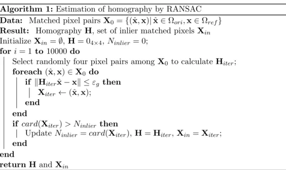
Thus, we need a robust method to select samples so that the matrix fits best the data set{(ˆx, x)} despite of undesirable effects. We apply here a popular method named RANSAC (random sample consensus) [FB87]. It is an iterative algorithm that each time extracts randomly a minimum number of data to calculate model. It selects inliers by filtering data set members according to an acceptable error threshold. The model with largest number of inliers is finally selected as best choice. In our case, the data set indicates {(ˆx, x)} and we select every time four samples to calculate the model H using the DLT method ([HZ03], chapter 3). The error to estimate is ∥Hˆx − x∥.
Both problems of noise and outliers are resolved by this algorithm. The design of error threshold εransacdefines a tolerance of noise and the selection of candidate
Algorithm 1: Estimation of homography by RANSAC Data: Matched pixel pairs X0 ={(ˆx, x)| ˆx ∈ Ωori, x∈ Ωref}
Result: Homography H, set of inlier matched pixels Xin
Initialize Xin=∅, H = 04×4, Ninlier = 0;
for i = 1 to 10000 do
Select randomly four pixel pairs among X0 to calculate Hiter;
foreach (ˆx, x)∈ X0 do
if ∥Hiterxˆ− x∥ ≤ εg then
Xiter← (ˆx, x);
end end
if card(Xiter) > Ninlier then
Update Ninlier= card(Xiter), H = Hiter, Xin = Xiter;
end end
return H and Xin
area as big as possible. Since we assume that background takes up most area of image, the output H belongs certainly to the planar background.
Remark that a set of inlier pixel coordinates Xinis also derived from Algorithm1.
They are pixel positions of scene shared by both aligned image and referential image and will be used for photometric correction in Chapter 4.
3.2.3 Reconstruction and interpolation
Having obtained the homography H between two images, we create in the end an aligned image defined on pixel grid Ωref of referential image. The RGB values
of pixels in aligned result is obtained by searching related pixel values in image to be aligned.
Figure 3.2: Problem of inverse mapping. the purple grid in original image and the blue grid in aligned image represent respectively Ωori and Ωref
with definition of RGB vectors. The blue grid in the original image is the inverse mapping result of Ωref. Its elements rarely superpose on Ωori. As an
example, the point xal∈ Ωref is mapped to ˆxal under H−1 with no definition
We define here the RGB vector of image to be aligned as Iori(xori)∈ {0, . . . , 255}3,
xori∈ Ωori (resp. Ial(xal)∈ {0, . . . , 255}3, xal∈ Ωref for its aligned result).
In order to get pixel values of xal ∈ Ωref, we need to know its related position
in image to be aligned. Since H is a non-singular matrix, we set up an inverse mapping and find out: ˆxal = H−1xal in image to be aligned. However, ˆxal is
very likely to be a position out of Ωoriand there is no such a definition of RGB
vector as: Iori(ˆxal), ˆxal̸∈ Ωori. A graphical description is shown in Figure3.2.
Figure 3.3: Inverse map-ping point and its surround-ing. ˆxal is inverse mapping
re-sult within scope of Ωori. It is
surrounded by four pixels defined on grid associated with RGB vec-tors xori1, xori2, xori3 and xori4.
This problem is solved by interpolating the RGB vector at ˆxal according to
its surrounding RGB values on the grid. In our application, we use a bi-linear interpolation to estimate the value of each vector Iori(ˆxal). For the no-edge areas,
we assume that an inverse mapping result ˆxal = (ˆxal, ˆyal), 1≤ ˆxal ≤ Mori, 1≤
ˆ
yal≤ Nori is within the scope of Ωori. It exists four pixels xori i = (xori i, yori i),
i∈ {1, 2, 3, 4} on grid Ωoriin the neighborhood of ˆxal as is shown in Figure 3.3
that relate to each other according to:
xori1+ 1 = xori2= xori3+ 1 = xori4;
yori1+ 1 = yori2+ 1 = yori3 = yori4.
Iori(ˆxal) is computed by two linear interpolations in both directions x and y with
the value of these pixels. If we interpolate at the first step the value in direction of x, we get two results at (ˆxal, yori1) and (ˆxal, yori3) as:
Iori(ˆxal, yori1) = xori2− ˆxal xori2− xori1 Iori(xori1) + ˆ xal− xori1 xori2− xori1 Iori(xori2); Iori(ˆxal, yori3) = xori4− ˆxal xori4− xori3 Iori(xori3) + ˆ xal− xori3 xori4− xori3 Iori(xori4).
In a similar way, we get the final result by another interpolation in the direction y as is presented by Function (3.5) ( [[ ]] means keeping integer part of result). Iori(ˆxal) = Iori(ˆxal, ˆyal) = [[ yori3− ˆyal yori3− yori1 Iori(ˆxal, yori1) + ˆ yal− yori1 yori3− yori1 Iori(ˆxal, yori3)]]. (3.5)
The obtained RGB vector is finally defined as RGB vector in aligned result: Ial(xal) := Iori(H−1xal) = Iori(ˆxal).
3.3
Experiments
Our experiments are carried out by repeating the alignment process between a reference image and every other images in the sequence. The reference image in Algorithm 2 refers to the first image in the sequence. In examples we show at the end of this chapter, the reference images are pre-cut and only their areas of interest are put into use. This pre-processing is not essential while it ensures the concentration of matched pixels on the plane, which is an important factor for the proper operation of RANSAC.
Algorithm 2: Geometrical alignment
Data: A set of n images Φori={Iori i(Ωi)}, i ∈ {1 . . . n}
Result: A set of geometrical aligned result Φal={Ial i(Ω1)}, i ∈ {1 . . . n}
Initialize Φal=∅;
Φal← Iori 1(Ω1);
foreach Iori i(Ωi)∈ Φori\Iori 1(Ω1) do
Compute matched pixels {(ˆx, x)|ˆx ∈ Ωi, x∈ Ω1} through SIFT estimation
on Iori i(Ωi) and Iori 1(Ω1);
Calculate homography H mapping Ωori i to Ωori 1 (see algorithm 1);
Re-sample Iori i on Ω1 by bi-linear interpolation of each channel as Ial i(Ω1);
Φal← Ial i(Ω1);
end
return Φal
Since the algorithm is very classical and has been used in many previous works, its correctness is no need to be proved. However, there are some details to notice in actual use.
First, the assumption on homography is easy to break down due to the optical aberration introduced by the camera lenses. To reduce the potential effects of the aberration, we take either of the following measures during our experiments: a) We use a prime lenses of good quality. The aim is to reduce geometrical aberration which results in the lose of rigidity of objects in images. It appears either as pincushion or as barrel shape which depends strongly on the zoom of lens. A poor quality of lenses will aggravate this phenomenon. We use a prime lens (SIGMA 30mm f1.5 DC HSM) to take most of our photos.
b) We arrange our target planes in the center of image. The distortion of view has the tendency to be more and more serious from the center to the side of a lens. We put therefore our interest objects in the center.
c) We take pictures with a modest change of camera positions. That means the reference image has less difference of visual angle with other images. In this way, the projection errors will be small even under the existence of distortion. The adjustment of parameters is another key point to the success of this pro-cess. The iteration number of RANSAC should be decided by the matched pixel numbers and the inlier probability which are difficult to predict. The best combi-nation of samples may not be included and the model may be inaccurate without enough iteration. To simplify the problem, we set it at a large number (10000). It makes the process slow while provides enough sampling in every cases. Be-sides, the relative threshold between nearest and second nearest neighbors in SIFT matching is set to 15 and the threshold of residual errors is set at 1 pixel. These thresholds are rather strict while in actual tests we get usually about 500 pairs of matched pixels for an image of size 1000× 2000, which are enough for our estimation.
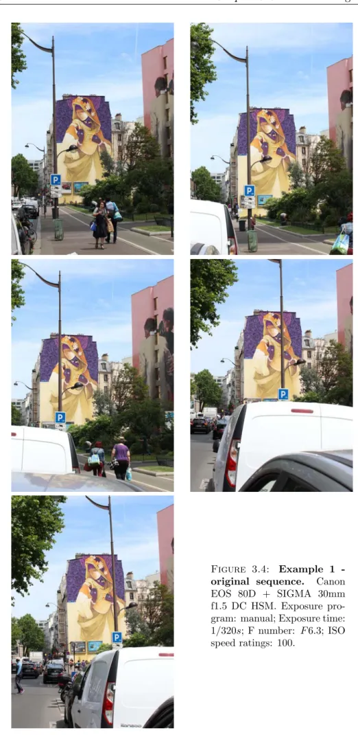
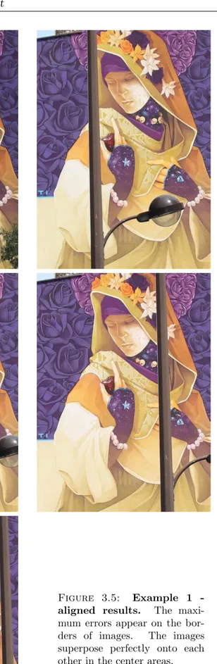
Based on the discussion above, we tested our program with several image se-quences and we give here three examples in Figures3.4,3.6,3.8along with their results: Figures3.5,3.7,3.9. The first images in original sequences are set as the reference and a direct cut-off of these images are presented as the first images in aligned results. Other images are resampled according to their vision and range. The results turn out to be satisfying. Most of the images superpose perfectly onto each other with errors below one or two pixels which are acceptable for the correct operation of further steps. We will see more challenging sequences (e.g.acquired by smart phone) in Part III.
Of course, these observations are based on the ideal condition supported by the perfect equipments. We will see errors occur with an increasing trend from the center to the border of image when using lenses of poor quality or with zoom. A further discussion will be later found in Chapter 7.
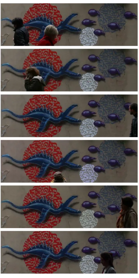
Figure 3.4: Example 1 -original sequence. Canon EOS 80D + SIGMA 30mm f1.5 DC HSM. Exposure pro-gram: manual; Exposure time: 1/320s; F number: F 6.3; ISO speed ratings: 100.
Figure 3.5: Example 1 -aligned results. The maxi-mum errors appear on the bor-ders of images. The images superpose perfectly onto each other in the center areas.
Figure 3.6: Example 2 - original sequence. Canon EOS 80D + SIGMA 30mm f1.5 DC HSM. Exposure program: manual; Exposure time: 1/100s; F number: F 6.3; ISO speed ratings: 160.
Figure 3.7: Example 2 - aligned results. The aligned results show no obvious errors in the center. The errors appear generally on the borders of images. The maximum errors are under 2 pixels.
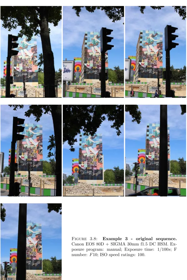
Figure 3.8: Example 3 - original sequence. Canon EOS 80D + SIGMA 30mm f1.5 DC HSM. Ex-posure program: manual; ExEx-posure time: 1/100s; F number: F 10; ISO speed ratings: 100.
Figure 3.9: Example 3 - aligned results. The maximum aligned errors are about 1 pixel. The distribution of maximum errors does not concentrate on certain areas.
Photometric Adjustment
Having been registered, every images in sequence convey the similar background pixels at the same positions. Yet due to the existence of color mismatches, these images can not be directly put into use for fusion procedure. The photometric difference between images is a common phenomenon which may be caused by many factors. The most possible reasons are listed as follows:
a) A variation of white balance adjustment caused by lighting con-dition changes (e.g.clouds, shadow of moving objects).
b) Changeable reflected lights from non-Lambertian objects under different observing angles.
c) Effects of spatial chromatic aberration and vignetting on lenses. d) Automatically changed camera parameters (aperture size, time
of exposure, ISO sensitivity) according to scene.
e) Unknown effects of camera processing (e.g.noise filtering, white balance, content enhancement) on different scenes.
In reverse, the effects of chromatic differences can be reduced by:
- capturing images in a short delay under stable illuminating conditions; - avoiding extreme viewing angles;
- applying professional cameras and optical lenses of good quality; - setting manually as many as possible the parameters (mode M)
- choosing file format with less automatic processing in camera (e.g.RAW) Even so, it is not possible to eliminate totally the problem and obtain pho-tometrically identical images. Without any adjustment, fusion results of such sequences risk being mottled, or even worse, bearing wrongly selected masks. We attempt thus to design a method to unify object colors in different images.
This chapter is dedicated to our discussion on color adjustment methods. It is arranged as follows: Section4.2introduces the pipeline of color formation process in camera. Section 4.3 includes our propositions of color alignment method. Finally, Section4.4provides experimental results of photometric correction along with our analysis on the performance of different approaches.
4.1
Experimental assumptions
In order to set up a stable model of luminance, we try to restrict the unpredictable effects of lighting conditions. At the stage of method conception, our experiences are carried out under three assumptions:
1) All surfaces obey Lambert hypothesis without great specular highlights. Lu-minance value remains the same regardless of observation directions.
2) Each group of images is taken in a short time to prevent changes of lighting conditions. Impacts of any unexpected factors are negligible.
3) Camera parameters such as aperture size, ISO value and shutter speed are fixed when taking an image sequence.
These requirements are easy to meet when taking photos of a matte surface with parameters fixed in a very short time. We suppose from then on that the luminance issued from the natural space remains approximately the same when it is received by camera at any positions.
Mathematically, we define the natural space as Πs ⊂ R3. We denote the
lumi-nance values, issued from xs∈ Πs, received by camera at two different positions
by L1(xs) and L2(xs). Their relationship may be expressed as:
L1(xs) = L2(xs) + εs(xs). (4.1)
where εs is a small value. The luminance will be further quantified and finally
mapped onto a 2D image grid after a complicated transformation through the optical and electronic systems in digital camera.
4.2
Color formation process in digital camera
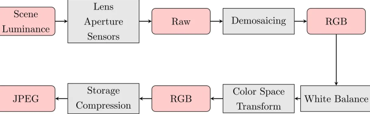
Every manufacturers have their own image processing algorithms, but they tend to share a rather fixed pipeline for color adjustment. Neglecting some procedures
for noise and artifacts removal, we present the major steps along with their output formats in Figure4.1.
In this section, we shall introduce each step of the pipeline and make clear of its role in color formation process. Generally speaking, most procedures, other than an optional sRGB transformation, are approximately linear. Therefore, as later we shall see, the conversion from scene luminance to digital RGB image can be approximately modeled by matrix.
Scene Luminance Lens Aperture Sensors Raw Demosaicing RGB White Balance Color Space Transform RGB Storage Compression JPEG
Figure 4.1: Pipeline of camera processing. Gray blocks represent main steps during camera processing while pink blocks indicate data formats after corresponding steps. There are also some manufacturers who put white balance in front of demosaicing, but it makes no big difference later in image color model because both steps are approximately linear.
4.2.1 From luminance to raw
Information of scene is firstly recorded by raw file. It is the most elementary image format that contains almost unprocessed data from the camera sensor ([M+17] Chapter 8). To state briefly this step, the scene luminance passes through a color-filter system then hits on a sensor array. Sensors convert pho-ton energy into intensity values after a series of analog and digital conversions such as sampling and quantization. The result is finally recorded by raw files (usually on 8 to 14 bits), whose data preserves as closely as possible information of natural scene. Most adjustments are carried out based on this original image format.
If we denote intensity value (red, green or blue) at position x by U (x)∈ R, the response function that projects luminance of 3D scene space to raw data on a 2D image grid Ω is approximately linear unless the signal is too weak or the sensor is saturated (see e.g.[Ham13] for CCD sensors):
Here, G is the ISO sensitivity function of camera that represents global gain of the whole acquisition process. The black level B is a value purposely added in the result by camera manufacturers in order to keep it positive. The term n is additive noise with respect to Gaussian distribution [ADGM14].
4.2.2 From raw to RGB
The sensor we mentioned above consists of a color filter array (CFA) on top of CCD or CMOS elements. Taking Bayer filter as an example, it is the most commonly used CFA in camera (see Figure4.2). A periodic pattern of red, green and blue filters separates light elements according to their wavelength range. The raw file, which records the color information received by sensors, presents therefore the image by mosaic of red, green and blue intensities.
Figure 4.2: Example of Bayer filter array. [Wik06] It is the three-color filter layer covering a sensor array (gray grid). Incoming light is decomposed into blue, red and green elements. The filter leaves element of its own color passing through its layer and arriving at sensor array. These sensors record then intensity of light and output an image called Bayer pattern image in Raw file. It requires a further demosaicing process to become a full-color image.
The part of work to compute a full-color image from the mosaic of three pri-mary colors is known as demosaicing. Many algorithms [ZW05,CC06,BCMS09, Get12] have been proposed to accomplish this conversion, and most of them share the idea of interpolation. Hence, this process is often approximately regarded as a linear conversion.
Following Function (4.1), we further assume the approximate equality of RGB vectors between images after demosaicing. We define respectively two digital images on grid Ω1 and Ω2. If a point xs ∈ Πs is mapped on these images at
x∈ Ω1 and ˆx∈ Ω2, the RGB vectors after demosaicing of these two pixels are
related by (εrgb is a small value):