HAL Id: hal-00312705
https://hal.archives-ouvertes.fr/hal-00312705
Submitted on 25 Aug 2008
HAL is a multi-disciplinary open access
archive for the deposit and dissemination of
sci-entific research documents, whether they are
pub-lished or not. The documents may come from
teaching and research institutions in France or
abroad, or from public or private research centers.
L’archive ouverte pluridisciplinaire HAL, est
destinée au dépôt et à la diffusion de documents
scientifiques de niveau recherche, publiés ou non,
émanant des établissements d’enseignement et de
recherche français ou étrangers, des laboratoires
publics ou privés.
Interactively solving school timetabling problems using
extensions of constraint programming
Hadrien Cambazard, Fabien Demazeau, Narendra Jussien, Philippe David
To cite this version:
Hadrien Cambazard, Fabien Demazeau, Narendra Jussien, Philippe David. Interactively solving school
timetabling problems using extensions of constraint programming. Practice and Theory of Automated
Timetabling V, Springer, pp.190-207, 2005, Lecture Notes in Computer Science, �10.1007/11593577�.
�hal-00312705�
Interactively solving school timetabling problems
using extensions of constraint programming
Hadrien Cambazard1, Fabien Demazeau2,
Narendra Jussien1 and Philippe David1
{hcambaza,jussien,pdavid}@emn.fr, [email protected]
1 ´
Ecole des Mines de Nantes, LINA CNRS
4 rue Alfred Kastler – BP 20722 - F-44307 Nantes Cedex 3, France
2
ISoft Chemin de Moulon 91190 Gif sur Yvette
Abstract. Timetabling problems have been frequently studied due to their wide range of applications. However, they are often solved manually because of the lack of appropriate computer tools. Although many ap-proaches mainly based on local search or constraint programming seem to have been quite successful in recent years, they are often highly dedi-cated to specific problems and encounter difficulties to take the dynamic and over-constrained nature of such problems.
We were confronted with such an over-constrained and dynamic problem in our institution. This paper deals with a timetabling system based on constraint programming with the use of explanations to offer a dynamic behaviour and to allow automatic relaxations of constraints. Our tool has successfully answered the needs of the current planner by providing solutions in a few minutes instead of a week of manual design. We present in this paper the techniques used, the results obtained and a discussion on the effects of the automation of the timetabling process.
1
Introduction
Timetabling problems have been frequently studied because of their wide range of applications. Scheduling activities occur in any human organisation and be-come quickly critical for large administrations. However, timetabling problems are often solved manually because of the lack of appropriate computer tools. Although many approaches mainly based on local search or constraint program-ming seem to have been quite successful in recent years, they are often highly dedicated to specific problems. This is due to the wide variety of problems which differ for example for education timetabling between schools, universities, engi-neering schools and more specific educational institutions. Among those prob-lems, two main difficulties are encountered: first, timetabling problems are often over-constrained and optimization criterias are hard to define. The optimization objective is often hard to express for the scheduling office itself because of the confusion induced by the manual process of resolution. Second, they are intrin-sically dynamic: activities, resources or constraints are sometimes unknown or
can often change at the last moment.
We were confronted with such an over-constrained and dynamic problem in our institution. We took the opportunity to experiment with PaLM [14], our ex-planation based constraint solver, in a real world situation. The system is based on constraint programming with the use of explanations [15] to offer a dynamic behaviour (the problem is not solved again from scratch when constraints are added or removed) and to allow an automatic relaxation of constraints in case of over-constrained problems. The tool has already been introduced for solving dynamic RCPSP (Ressource Constrained Project Scheduling Problems) in [9]. Experiments on academic problems such as the RCPSP encouraged us to apply the technique in a real world situation. Our tool has successfully answered the needs of the planner by providing solutions in a few minutes instead of a week of manual computation.
This paper is organized as follows: Section 2 introduces the timetabling prob-lem we solved. Formal models are then presented in Section 3: a linear and a constraint formulation are given. Section 4 presents the basics of explanation-based constraint programming and our results are discussed in Section 5.
2
Problem description
The problem was met in a French engineering school: the ´Ecole des Mines de Nantes (EMN). EMN offers a 4-year program which consists of a 2-year common core followed by 2 specialized years. There are 9 possible specializations in various areas of study like computer science, production and logistics, environment or management (a complete list is provided in table 1). EMN tries to offer as much choice as possible to its students.
In this paper, we report our work on the third year timetabling problem. All students are supposed to choose a major and a minor (among the nine possible specializations) and a set of open courses. The idea is to let them finalize their choices for their final year where either the major or the minor becomes the only set of courses that they follow. Notice that the choice of a specialization implies a fixed set of required courses. The task is to design a weekly timetable which will be in use for a complete semester. Each course available for the studied semester is to be assigned to a half-day slot during the week. The main problem is to determine which courses will happen simultaneously. The aim is to allow as many students as possible to attend all the required courses of their two choices and as many as possible of their free choices. Each option3is defined by two sets
of required courses (depending if the topic is a major or a minor).
3
An option is a topic or an area of study chosen by a student to specialize in during his last year.
2.1 Static part of the problem
The built timetable must verify a given set of constraints. Both hard and soft constraints can be defined. Hard constraints are as follows:
– topic availability: required courses of each topic have to be assigned non overlapping slots ;
– pre-requisite: some courses are pre-requisite for others and must therefore take place in different slots ;
– room availability: a maximum number of courses is allowed simultaneously because of room limitations
The provided timetable must meet all these hard constraints. Moreover, soft constraints are highly desirable for a useable timetable:
– teachers’ availability: teachers can specify their availability on given slots during the week
– major/minor selection: for each student, the major and minor required courses should be scheduled in non overlapping slots.
– free course selection: additional courses chosen by a given student must fall in different slots.
Although no precise preference function is defined, the person in charge first tries to satisfy teachers as much as possible (many teachers come from other schools or universities) and to leave students free to attend their major/minor choice. Secondly, the objective is to fulfill the other students’ requests in order to provide each of them with a conflict-free schedule. The main problem consist in optimizing both objectives:
1. minimize the number of violated pairs of options (major/minor); 2. minimize the number of violated pairs of courses4.
For the first semester, the priority is given to the number of pairs of options available and for the second semester, it consists in minimizing the number of conflicts between courses5.
Typical instances for the first semester of the third year in EMN involve 120 students, 30 different courses, 9 main topics and 7 courses per student. The 30 courses have to be assigned in 7 timeslots. Notice that, even if the number of courses and students is quite small compared to typical universities, the student schedule is complete. 72 pairs of options are possible, 3 courses are required for a major and 2 for a minor. Around 30 pairs among the 72 are effectively chosen by students and the distribution of option over the pairs is varied. We cannot predict a priori that any two options will never be together. For example, environment and computer science options are not incompatible (a particular in-stance can be seen on table 1). Therefore, the problem is often over-constrained
4 Violated pairs of options and courses will be denoted as conflicts in the latter. 5
Optimization was not required at the beginning by the planner and became possible once the satisfaction of hard constraints had been successfully taken into account.
only considering the soft constraints concerning major/minor selection.
The student scheduling problem [4] (SSP) has the same objective: providing conflict-free schedules. Students need to be assigned to courses in the classical SSP (the timetable is already done) whereas our problem consists in assigning courses to timeslots (the timetable is built according to student’s requests). A similar problem is solved in [22] where a feasible and personalized weekly timetable is assigned to every student of a Spanish Engineering School. But in this case again, several groups have been already done for every subject, every group has a fixed timetable and is already scheduled to lecturers. Actually, our problem can be seen as a specific demand driven timetabling problem [4] where the number of satisfied course requests is to be maximized.
P P P P P PP Major Minor
OMIT CSE EG CSAD QRS OMPL ACC NT ESE OMIT - 7 1 4 1 10 0 0 0 CSE 4 - 0 13 0 0 2 0 0 EG 1 0 - 0 2 0 0 3 5 CSAD 0 6 2 - 0 1 1 0 0 QRS 0 0 0 0 - 7 0 0 1 OMPL 2 0 4 0 13 - 2 0 1 ACC 4 3 1 0 2 9 - 1 3 NT 1 0 4 0 0 0 0 - 2 ESE 0 0 4 0 0 0 0 1
-Table 1. The allocation of minor and major choices in a particular instance (the pair (ACC,QRS) has been chosen by two students for instance). Options are the following: Computer systems engineering (CSE), Computer science as an aid to decision-making (CSAD), Organisation and management of information technologies (OMIT), Auto-matic control and industrial computation (ACC), Operations management in produc-tion and logistics (OMPL), Quality and reliability of systems (QRS), Environmental engineering (EG), Energetic system engineering (ESE), Nuclear and associated tech-nologies (NT).
2.2 Dynamic part of the problem
One of the main requirements from the scheduling office was the possibility to quickly change a previous solution in order to take unexpected events into account. Constraints concerning the students are supposed to be quite static, even if the timetabling can be computed whereas some student choices are still missing. The dynamic part of the schedule is more related to logistic problems and unexpected events concerning:
– The link with timetabling of other years (the four years share common re-sources: rooms, equipment for practical sessions but also teachers)
– The requirement of the teachers (insiders and specially outsiders)
It is for instance usual that the availability of an outside contributor to a course remains unknown until the last moment. Moreover, as teachers are involved in courses for different years whose timetables are not scheduled at the same period, unexpected constraints concerning teachers occur frequently. The dynamic changes considered here focus on addition of constraints (teachers availability or logistic needs). Literature on dynamic timetabling is not very rich. However, our dynamic changes are related to the minimal perturbation problem which consists in incorporating the changes, along with the initial solution, as a new problem whose solution must be as close as possible to the previous one. [18] proposes a local search method on partial feasible assignments guided by conflicts statistics to solve the minimal perturbation problem. Our approach is quite different but also pragmatic (see 4.3). However, recent dedicated complete methods can also be found in [1].
3
Formal Models
The input data for a given timetable are the following:
– Courses = {1, 2, ..., n}; – Options = {1, 2, ..., o}; – Students = {1, 2, ..., m};
– ∀i ∈ Options, Requisite1i⊂ Courses;
– ∀i ∈ Options, Requisite2i⊂ Courses;
– ∀s ∈ Students, Choicess⊂ Courses
– R is the maximum number of free rooms in a each timeslot; – NP is the number of time periods in a week;
– wi1i2 denotes the conflicts associated to a pair of courses (i1, i2) (for
exam-ple, the number of students that took the pair (i1, i2)).
Let Courses be the set of courses, Options be the set of options, Requisite1i
be the first set of required courses for option i and Requisite2i, the second set
of required courses for the same option i. For each student s, the inputs are his major and minor O1s,O2s and his free choice of courses F reeCoursess ⊂
Courses. Therefore, the complete set of courses, Choicess, corresponding to a
student s is equal to Requisite1O1s∪ Requisite2O2s∪ F reeCoursess.
3.1 A Linear Programming model
A linear model can be expressed using boolean variables xijwhich take the value
1 if the course i is placed in the timeslot j and 0 otherwise.
Integrity constraints:
Each course must be placed exactly once: ∀i ∈ {1..n}, P
jxij= 1
Hard constraints:
Option validity: ∀o ∈ Options, ∀j ∈ {1..NP } P
i∈Requisite1oxij ≤ 1
Linked courses: ∀i1, i2 pre-requisite, ∀j ∈ {1..NP } xi1j+ xi2j ≤ 1
Room availability: ∀j ∈ {1..NP } P
i∈Coursesxij ≤ R
Soft constraints:
Teachers’ availability: teacher of course i
is absent at period p, xip= 0
Option choice: ∀s ∈ Students,
∀j ∈ {1..NP }, P i∈ Requisite1O1s ∪Requisite2O2s xij≤ 1
Course choice: 6 ∀s ∈ Students,
∀j ∈ {1..NP }, P
i∈Choicesxij ≤ 1
This model corresponds to the problem as it was first expressed by the scheduling office. Theses requirements were modified to consider an optimiza-tion model which minimizes the number of conflicts once the problem has been proved to be over-constrained. An optimization function could be added using yi1,i2 boolean variables to express the fact that the courses i1and i2are placed in
the same timeslot. An optimization function could be written (with appropriate channelling constraints to link x and y variables):
M in X
(i1,i2)∈Courses×Courses
yi1j2× wi1,i2
3.2 A constraint programming model
Constraint programming (CP) techniques have been widely used to solve schedul-ing problems. A constraint satisfaction problem (CSP) consists of a set V of variables defined by a corresponding set of possible values (the domain D) and a set C of constraints. A solution for the problem is an assignment of a value to each variable such that all the constraints are simultaneously satisfied. The constraints are handled through a propagation mechanism which allows the re-duction of the domains of variables and the pruning of the search space. The propagation mechanism coupled with a backtracking scheme allows the search space to be explored in a complete way.
CP seems a good approach to our problem as almost all the constraints described
6
This constraint includes the previous one but the distinction will be made for relax-ation.
here fall within difference constraints (except room availability) i.e. courses that cannot be scheduled into the same period. We can therefore enforce our model by using global constraints like the alldifferent [19] or global cardinality7 [20]
constraints. Such constraints constitutes an efficient way to handle recurrent patterns or sub-problems, they contain complex algorithms able to efficiently prune large portions of the search space.
The constraint model proposed uses n integer variables xidenoting the
times-lots in which courses i are scheduled.
∀i ∈ {1..n}, domain(xi) = [1..NP ]
Hard constraints can be simply written as follows:
Option validity: ∀o ∈ Options, alldiff erent(xi|i ∈ Requisite1o)
Linked courses: ∀i, j linked courses, xi6= xj
Room availability: gcc({xi|i ∈ Courses}, {0|(1..NP )}, {R|(1..NP )})
Soft constraints:
Teachers’ teacher of course i
availability: is absent at period p, xi6= p
Option choice: ∀s ∈ Students, alldiff erent(xi|i ∈ Requisite1O1s
∪Requisite2O2s
) Course choice: ∀s ∈ Students, alldiff erent(xi|i ∈ Choices)
One can first notice that the problem is highly symmetrical. In fact, disre-garding the teachers’ availability constraints, two timeslots are interchangeable. A partial assignment of at least two timeslots is equivalent by exchanging the slots. When the search algorithm has proven that one assignment is inconsistent, it is a waste of effort to try the equivalent permuted assignment.
The problem can be seen as a generalized assignment problem (GAP). It is a well-known NP-complete combinatorial optimization problem which consists of assigning a set of tasks (courses) to a set of resources (half-day timeslots). But it can also be considered as a weighted CSP which minimizes the weighted sum of unsatisfied constraints (by considering a weight for each soft constraint). The weight wi1,i2 can be associated to each elementary difference xi1 6= xi2.
Coefficients can be added to distinguish minor choice and free courses choices. However, our goal was firstly to provide a solution to hard constraints and, as requested by the planner, to quickly re-compute a solution in case of changes (often concerning teachers) or to simulate different scenarii with unknown data. The dynamic and over-constrained aspect of the problem led us to consider constraint programming with specific enhancements: explanations.
7 It is denoted by gcc(X, lb, ub) where X is a set of variables, lb and ub, two sets of
integers where lbiand ubigives the minimal and maximal number of times the value
4
Explanations for constraint programming
Solving dynamic constraint problems has led to different approaches. Two main classes of methods can be distinguished: proactive and reactive methods. On one hand, proactive methods propose to build robust solutions that remain solu-tions even if changes occur. On the other hand, reactive methods try to reuse as much as possible previous reasonings and solutions found in the past. Reactive methods avoid restarting from scratch and can be seen as a form of learning. One of the main methods currently used to perform such learning in dynamic constraint solving is a justification technique that keeps trace of inferences made by the solver during the search. Such an extension of classical constraint pro-gramming has been recently introduced. It is called explanation-based constraint programming (e-constraints) and it has already proved its interest in many ap-plications [14] including dynamic constraint solving. One can refer to [9] to find an example of using explanations to solve timetabling problems. We recall in this section what explanation-based constraint programming is and how it can be used.
4.1 Definition
An explanation records information to justify a decision of the solver as a re-duction of domain or a contradiction. It is made of a set of constraints C0 (a subset of the original constraints of the problem) and a set of decisions, dc1,
dc2, ..., dcn, taken during search (eg the branching part of a branch and bound
algorithm such as x = a or x < y).
An explanation of the removal of value a from variable v will be written as follows:
C0∧ dc1∧ dc2∧ · · · ∧ dcn⇒ v 6= a
An explanation e1is said to be more precise than e2if and only if e1⊂ e2. The
more precise the explanation, the more relevant the learning about the inference is. When a domain is emptied, a contradiction is identified. An explanation for this contradiction is computed by uniting each explanation of each removal of value of the variable concerned. At this point, intelligent backtracking algorithms that question a relevant decision appearing in the conflict are conceivable [5]. By keeping in memory a relevant part of the explanations involved in conflicts, a learning mechanism can be implemented [16]. Notice that a nogood is associated to any explanation: dc1∧ dc2∧ · · · ∧ dcn∧ v = a.
4.2 Computing explanations
During propagation, constraints are awaken (like agents or daemons) each time a variable domain is reduced (this is an event) possibly generating new events (value removals). A constraint is fully characterized by its behaviour regarding the basic events such as value removal from the domain of the variables and domain bound updates. Explanations for events are computed when the events are generated.
Explanations for basic constraints. It is easy to provide explanations for basic constraints. The following example shows how to compute them.
Example 1. Let us consider a two-variable toy problem: x and y with the same set of possible values [1, 2, 3]. Let us state the constraint x > y. The resulting sets of possible values are [2, 3] for x and [1, 2] for y. An explanation for this situation is the constraint x > y. Now, let us suppose that we choose to add the constraint x = 2. The only resulting possible value for x is 2. The explanation of the modification is the constraint x = 2. The other consequence is that the remaining value for y is 1. The explanation for this situation is twofold: a direct consequence of the constraint x > y and also an indirect consequence of constraint x = 2.
Precise explanations for global constraints. Computing a precise expla-nation for global constraints may not be easy because it is necessary to study the algorithms used for propagation. However, there always exists a generic ex-planation: the current state of the domains of each variable of the constraints. [21] describes how to provide precise explanations for the all-different constraint involved in our timetabling problem.
4.3 Explanations for handling dynamic problems
Incremental constraint addition to a problem is a well-known issue in classical constraint programming solvers: it is often the usual way constraints are added to the constraint system. However, incremental constraint retraction is not so easy. Several extensions have been proposed to handle dynamic retraction of constraints: some of them [2, 12] analyze the reduction operators to be able to determine the past effects of a constraint and so incrementally retract it; others, following [3], store information to achieve that determination.
Explanations (or simplifications) may be used as past effect determination tools [6, 15].
Dynamic constraint retraction. Dynamic constraint retraction of a con-straint c can be achieved through the following steps in an explanation-based system:
1. Disconnecting The first step is to remove the retracted constraint c from the constraint network (no further propagation).
2. Setting back values The second step is to undo the past effects of the constraints, both the direct (each time the constraint operators have been applied) and indirect (further consequences of the constraint through oper-ators of other constraints) effects of that constraint. We can easily put back in its domain, each value whose explanation contains the constraint. Past events are recorded in explanations.
3. Re-propagate It is finally necessary to re-propagate in order to reach a consistent state. As our explanations are neither minimal nor unique, many
ways exist to deduce the removal of a value and only one of those ways is stored in the current explanation. Therefore a new propagation is necessary.
Re-propagation of constraints. Although determining the past effects of a constraint c is quite easily done by referring to the explanations that do con-tain reference to c, efficient re-propagation is not provided in classical constraint solvers. Indeed, another event needs to be handled: value restoration (or bound restoration). Instead of calling a general local consistency operator for han-dling this new event, it is possible to design new operators dedicated to this re-propagation phase. One can refer to [7] for more details.
4.4 Solving over-constrained problems
Computing explanations for conflicts and for incrementally removing a constraint from a constraint system leads to over-constrained problems.
Consider the classical enumeration process used to solve CSP as a dynamic se-quence of constraint additions (assigning variables) and retractions (backtracks). We can apply a simple strategy [15]: solve the complete constraint system as usual and, if necessary (i.e. once the problem has been proven over-constrained), use the conflict explanation to identify the next constraint system to consider (using a comparator [23] that takes into account the user’s preferences) and per-form the constraint modification (retraction(s) and/or addition(s)) incrementally still using explanations. This process is iterated as long as no suitable solution is found. The use of the comparator guarantees the optimality of the solution. Section 5.3 explains in more details how this process leads to an optimization with respect to soft constraints.
Notice that search is made in the space of possible relaxations in opposition to the space of possible assignments in more classical approaches. We can carry this idea further and imagine a local search process in the space of possible relaxations (see Section 5.3).
5
Solving dynamic timetabling problems
5.1 An interactive tool
Our system has been implemented using PaLM [14] and the Java Swing API to design the graphical interface. PaLM is launched as a background process and waits for dynamic events: addition, retraction of constraints or asking of a new solution (during search, the graphical user interface is locked). As the success of the tool was largely depended on a user-friendly interface as well as the ability to solve the problem, we paid a particular attention to the planner’s needs and her manual process.
A screenshot of the implemented system can be seen on picture 1. One can see a classic timetable representation with 7 timeslots and 30 courses. Each line
corresponds to a timeslot. Boxes on the left column give information on the com-plete timeslot (number of conflicts and number of involved students). Inside a timeslot, courses are ordered according to the number of involved students (from warm to cold colours, dark to light on the picture). Each course corresponds to a box with the following information: conflicts with every other courses in the same slot, number of involved students, reference to the course and the kind of dynamic constraint added on it. Tool Tip texts help to know the purpose of each number by simply pausing with the cursor over it. Constraints can be added using a mouse left click on the course or the concerned timeslot. A new window allows the constraint and other courses or timeslots involved to be se-lected. The current state of dynamic constraints added since the beginning is also maintained, allowing easy removals.
The automated timetabling system implemented met the requirements of the scheduling office by proposing the following features:
– A dynamic behaviour. 3 kinds of constraints can be added or removed: equal-ity, difference and alldifferent, either between courses or courses with times-lot. By dynamically adding, retracting constraints or changing their weight, the planner is able to perform simulations on the solution, to evaluate its robustness and to manually build (in interaction with the tool) good solu-tions.
– A complete visualization of conflicts in each timeslot and for each course with its neighbours offers the possibility to make judicious dynamic changes to a solution. Previous indicators used by the planner in the manual process, such as the number of inactive students in a timeslot, have been included. Additional statistics on a solution are accessible through a menu to evaluate the results in more details.
5.2 Results
The first results were of great interest for the planner:
– The tool is able to provide better solutions quickly. A solution was found manually in a week when 10 solutions are now obtained in about 10 minutes. Moreover, solutions have a better quality than those found by hand even if no optimization is done. Nevertheless, the planner is forced to pre-allocate some courses to allow a quick computation of a solution. It is a simple way to reduce the symmetries of the problem. A good way of doing it consists in setting the required courses of the most chosen option in different slots, as they will not be found together in any conceivable good solution.
We compared the result during the start-up year of the tool and noticed that conflicts have been reduced by around 20 % on both semesters. Moreover, the number of students able to follow their minor choice has been increased by 3 % (it corresponds to a reduction of 10 % of the number of unsatisfied students concerning their minor). The tool was good enough to be accepted
by the scheduling office and since then, six semesters have been scheduled with it.
– Unexpected events, or unknown data can be taken into account quickly be-fore the start of the courses without changing the original solution too much. The system doesn’t provide any guarantee on the perturbation. It doesn’t ensure to get the minimal perturbation. However, the stability of a solu-tion has been analysed for scheduling problems in [8, 10, 11] using the same technique and proved to be quite effective.
– A simulation tool: The tool has been quickly used by the planner to simulate different situations. Common sense assumptions were made to make the manual scheduling process easier and are now questioned and simulated with the tool. For example, Human social science courses were often put together in the last timeslot considering that each student is forced to choose one course in this field. However, best solutions do not necessary respect such assumptions. Dynamic abilities intend here to take advantage of the know-how of the planner as much as possible because she remains a central element in the process of resolution.
5.3 Post optimization processing
When solving an instance by hand, the planner focused on the satisfaction of hard constraints and teacher wishes. As hard constraints have been successfully taken into account with the current system, the planner can focus more on student wishes. Once she was experienced with the tool, the time gained has been used to optimize the solution through a simulation process. We noticed how she brought her know-how into play to interact with the tool using its dynamic abilities and to focus on the optimization objective. It was a new aspect of her work since she was more focused on hard constraints in the past. It was therefore for us a second step of resolution.
Her manual process can be seen as a manual local search around the first solution given by the system and we came naturally to the point of automating the technique as a local search.
User preferences. Preferences are taken into account during the relaxation of constraints. When the problem has been proved over-constrained, we use the current contradiction explanation and the user preferences to identify the constraint to be relaxed. The use of a simple comparator8 [23] that considers
the constraint with the minimal weight ensures that the heaviest weight among the relaxed constraints is minimal in any solution. It guarantees the optimality of the solution according to this comparator. A configuration is defined by two sets of constraints (A, R) where A is the set of active constraints and R the set of relaxed constraints. A configuration C is said to be preferred to C0 according to a given comparator. In the previous case, two configurations are compared on
8
Fig. 1. A timetable with 7 timeslots and 30 courses. Light boxes on the left give information on the complete timeslot (number of conflicts and number of students concerned). In a timeslot, courses are ordered according to the number of students concerned (from warm to cold colours). Each course corresponds to a box with the following information: conflicts with every neighbours, number of involved student and the kind of added manual constraints. Tool Tip Texts help to know the purpose of each number. Nu m b er of confli cts bet w een Crypt ography and its t h ree neighbours. Num b er of involved students in t h e co urse
the heaviest weight of their constraints.
The solutions provided in this way are close to the planner’s objective and first solutions have shown to be good solutions. However, a more precise objective could be the minimization of the weighted sum of relaxed constraints.
Such a comparator needs all the contradiction explanations computed during the search to determine (each time a new contradiction occurs) the new set (of constraints) of minimal weight that covers every contradiction explanation. It leads to two main problems:
– The number of contradiction explanations can be exponential;
– Finding the set of minimal weight covering the whole set of explanations is an NP hard problem (set covering problem).
To overcome those problems and try to provide better solutions, we decided to perform local search techniques. This choice was directed by the well-known abil-ity of local search techniques to efficiently improve an initial solution generated using an heuristic method. However, a very different approach for performing the search has been tried using the dynamic abilities of our system.
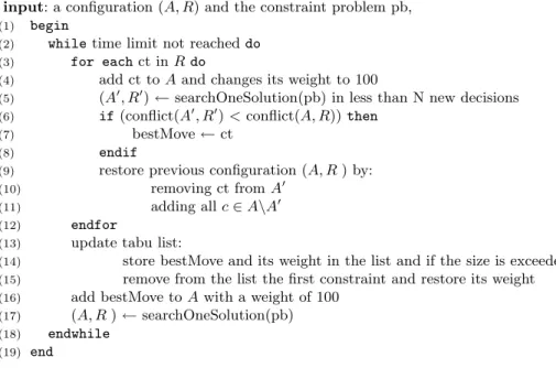
Local search in the space of configurations. Local search techniques can be seen as methods which iteratively apply simple moves to a solution. Among the wide variety of techniques, tabu search is a local metaheuristic which avoid en-trapment in local minima. It has already proved its interest in solving timetabling problems [13]. We use here one of the simplest forms of Tabu search without achieving an effective balance of intensification and diversification. But instead of performing the search on complete or partial assignments as usual, we per-form the search in the space of configurations using the dynamic abilities of an explanation-based constraint solver.
Let (A, R) be the configuration reached at the end of the first step of the search. As the use of a simple comparator gives good results, we start from this point a local search in a second step of resolution. The tabu search is performed by trying to add a constraint from R to A. The neighbour function (a move) consists therefore in adding a relaxed constraint to the set of active constraints. To avoid cycling, the weight of the constraint is dynamically changed to an in-finite value (in our case, 100). Adding a constraint with an inin-finite weight to A can lead to very difficult sub-problems. Therefore, to reduce the computational effort of each move, we limited the number of extensions (or backtracks, or re-pairs) allowed to find a new solution. Once the constraint of R leading to the best solution has been added to A, we store it in a tabu list with its original weight. As long as the constraint appears in the list, its weight stays infinite in the problem, forbidding its relaxation. When the constraint leaves the list, it takes back its original weight and becomes relaxable.
Local search methods traditionally encounter difficulties in taking hard con-straints into account. Notice that the solution provided here after each move sat-isfies hard-constraints because arc-consistency is maintained after each retraction
Tabu search:
input: a configuration (A, R) and the constraint problem pb,
(1) begin
(2) while time limit not reached do
(3) for each ct in R do
(4) add ct to A and changes its weight to 100
(5) (A0, R0) ← searchOneSolution(pb) in less than N new decisions
(6) if (conflict(A0, R0) < conflict(A, R)) then
(7) bestMove ← ct
(8) endif
(9) restore previous configuration (A, R ) by:
(10) removing ct from A0
(11) adding all c ∈ A\A0
(12) endfor
(13) update tabu list:
(14) store bestMove and its weight in the list and if the size is exceeded:
(15) remove from the list the first constraint and restore its weight
(16) add bestMove to A with a weight of 100
(17) (A, R ) ← searchOneSolution(pb)
(18) endwhile
(19) end
Fig. 2. Tabu search in configurations space
or addition of constraint. When no solutions are found for every constraint of R, we can decide to increase the number of extensions allowed or to stop the search.
The neighborhood of a configuration (A, R) is defined by transferring a con-straint from R to A, the computation of a consistent state with this move leads to relax some constraints from A to R. Therefore the configuration reached (A0, R0) can be far from the original one. The limitation of the number of extensions to re-compute a solution from the previous one ensures remaining in a close neigh-borhood of (A, R) and limiting the time needed to compute a move. Moreover, after proving that a move is not reachable in the limit of time allowed, it can be removed from the neighborhood until the current configuration has been changed enough. It is a waste of time of proving at each step that a move doesn’t not belong to the current neighborhood.
Results on optimization. The tabu is able to improve the first solutions by around 10 % on both semesters. It compensates one main problem of the simple comparator used by the solver to relax constraints: All the constraints of one level can be relaxed whereas only one constraint of a higher level needs to be relaxed to get a solution (it is called a flooding phenomenon). Table 2 summarizes the conflict on major/minor choices (option choices for the first semesters in column Opt ), the free choices in column Conflicts and the value of the optimization function considered to perform optimization.
Table 2. Results obtained on three years. Instances X1 corresponds to a first semester problem and instances X2 to a second semester.
Instances First Solution Tabu (5min) Opt Conflicts Obj. Fct Opt Conflicts Obj. Fct A1 6 162 282 5 138 238 B1 11 151 391 13 140 380 C1 7 160 320 5 133 273 Improvement: 10,3 % A2 - 54 54 - 49 49 B2 - 97 97 - 90 90 C2 - 117 117 - 103 103 Improvement: 9,7 %
6
Discussion
The tool can successfully solve the problem even if optimization is still an open question. Of course, as mentioned before, it is still necessary to pre-affect some courses by hand to reduce symmetries and to obtain an efficient resolution. We would like to insist on the fact that the tool is unable to replace the planner’s work. On the contrary, although a lot of progress has been made in this research field, timetabling problems remain very difficult and specific. Computer tools still need to be open and interactive to take advantage of the know-how of the planner. In our case, the tool has significantly changed her work and opened new perspectives. Common sense assumptions, needed when the problem is solved by hand (to reduce its complexity) can now be questioned and others evaluated. By executing thankless work, the tool gives freedom to the planner who can analyse the problem without any reductionist assumptions. Therefore, her understanding and way of doing it have considerably changed with the tool which gives efficient and relevant information about the problem. Only the planner knows what makes a good solution, has in mind the complete problem with its human dimension and is used to students and teachers’ behaviour. That is why an objective function is so hard to define clearly and the know-how of the planner so critical.
We have tried to develop an efficient tool based on recent technologies in order to answer precise needs, which is a quite different objective compared to the resolution of very hard and academic problems.
7
Conclusion and further work
We have presented in this paper a practical application of an explanation based system to solve a school timetabling problem. The system has proved its effi-ciency when it was accepted by the scheduling office. First, our intention was to show the interest of using explanation techniques to solve dynamic and over-constrained timetabling problem. Second, we presented a different local search
technique that tries to take advantages both of constraint programming for sat-isfying hard constraints and local search for its performance in an optimization context. We plan in the future to keep working on the problem itself as well as the tool:
– Our next step would be to improve the system with user-friendly expla-nations [17] to answer to legitimate questions of the planner such as: Why is the problem over-constrained ? Contradictions could be explained to the user by providing the explanation computed for the contradiction in a high level representation.
– Further experiments have to be done concerning the optimization process. After the local search phase, we intend to restart the search with the new upper bound. Efficient lower bounds and branching scheme will therefore be needed. A more precise study on the problem has to be carried out to evaluate the quality of the first solution found.
Even if work remains to understand the problem, these first results show that explanation constraint programming can be successfully integrated in a real-world situation.
Acknowledgments
The authors would like to thank Val´erie Kirion, in charge of timetabling of the third year students, for her help and collaboration.
References
1. Roman Bart´ak, Thomas M¨uller, and Hana Rudov´a. A new approach to modeling and solving minimal perturbation problems. In K.R. Apt, F. Fages, F. Rossi, P. Szeredi, and J. Vancza, editors, Recent Advances in Constraints, Lecture Notes in Computer Science, pages 233–249, Pittsburgh, 2004. Springer-Verlag.
2. Pierre Berlandier and Bertrand Neveu. Arc-consistency for dynamic constraint problems: A RMS free approach. In Proceedings ECAI’94 Workshop on Constraint Satisfaction Issues raised by Practical Applications, August 1994.
3. Christian Bessi`ere. Arc consistency in dynamic constraint satisfaction problems. In National Conference on Artificial Intelligence – AAAI’91, 1991.
4. Eddie Cheng, Serge Kruk, and Marc Lipman. Flow formulation for the student scheduling problem. In E. K. Burke and P. De Causmaecker, editors, Practice and Theory of Automated Timetabling IV, number 2740 in Lecture Notes in Computer Science, pages 299–309. Springer-Verlag, 2003.
5. Bruno de Backer and Henri B´eringer. Intelligent backtracking for CLP lan-guages: An application to CLP(R). In Vijay Saraswat and Kazunori Ueda, ed-itors, ILPS’91: Proceedings International Logic Programming Symposium, pages 405–419, San Diego, CA, October 1991. MIT Press.
6. Romuald Debruyne. Arc-consistency in dynamic csps is no more prohibitive. In 8 th Conference on Tools with Artificial Intelligence (TAI’96), pages 299–306, 1996.
7. Romuald Debruyne, G´erard Ferrand, Narendra Jussien, Willy Lesaint, Samir Ouis, and Alexandre Tessier. Correctness of constraint retraction algorithms. In FLAIRS’03: Sixteenth international Florida Artificial Intelligence Research Society conference, pages 172–176, St. Augustine, Florida, USA, May 2003. AAAI press. 8. Abdallah Elkhyari. Outils d’aide `a la d´ecision pour les probl`emes
d’ordonnancement dynamique. PhD thesis, ´Ecole des mines de Nantes, Nantes, France, 2003. in French.
9. Abdallah Elkhyari, Christelle Gu´eret, and Narendra Jussien. Solving dynamic timetabling problems as dynamic resource constrained project scheduling problems using new constraint programming tools. In E. K. Burke and P. De Causmaecker, editors, Practice and Theory of Automated Timetabling IV, number 2740 in Lecture Notes in Computer Science, pages 39–59. Springer-Verlag, 2003.
10. Abdallah Elkhyari, Christelle Gu´eret, and Narendra Jussien. Constraint program-ming for dynamic scheduling problems. In Hiroshi Kise, editor, ISS’04 Interna-tional Scheduling Symposium, pages 84–89, Awaji, Hyogo, Japan, May 2004. Japan Society of Mechanical Engineers.
11. Abdallah Elkhyari, Christelle Gu´eret, and Narendra Jussien. Stable solutions for dynamic project scheduling problems. In PMS’04 International Workshop on Project Management and Scheduling, pages 380–384, Nancy, France, April 2004. 12. Yan Georget, Philippe Codognet, and Francesca Rossi. Constraint retraction in
clp(fd): Formal framework and performance results. Constraints, an International Journal, 4(1):5–42, 1999.
13. Alain Hertz. Tabu search for large scale timetabling problems. In European Journal of Operations Research, number 54, pages 39–47, 1991.
14. Narendra Jussien. e-constraints: explanation-based constraint programming. In CP01 Workshop on User-Interaction in Constraint Satisfaction, Paphos, Cyprus, 1 December 2001.
15. Narendra Jussien and Patrice Boizumault. Best-first search for property mainte-nance in reactive constraints systems. In International Logic Programming Sym-posium, pages 339–353, Port Jefferson, N.Y., USA, October 1997. MIT Press. 16. Narendra Jussien and Olivier Lhomme. Local search with constraint propagation
and conflict-based heuristics. Artificial Intelligence, 139(1):21–45, July 2002. 17. Narendra Jussien and Samir Ouis. User-friendly explanations for constraint
pro-gramming. In ICLP’01 11th Workshop on Logic Programming Environments (WLPE’01), Paphos, Cyprus, 1 December 2001.
18. Thomas M¨uller and Hana Rudov´a. Minimal perturbation problem in course timetabling. In Proceedings of the fourth international conference on the Practice And Theory of Automated Timetabling (PATAT’04), pages 283–303, Pittsburgh, 2004.
19. J.-C. R´egin. A filtering algorithm for constraints of difference in CSPs. In AAAI 94, Twelth National Conference on Artificial Intelligence, pages 362–367, Seattle, Washington, 1994.
20. Jean-Charles R´egin. Generalized arc consistency for global cardinality constraint. AAAI / IAAI, pages 209–215, 1996.
21. Guillaume Rochart, Narendra Jussien, and Fran¸cois Laburthe. Challenging expla-nations for global constraints. In CP03 Workshop on User-Interaction in Con-straint Satisfaction (UICS’03), pages 31–43, Kinsale, Ireland, September 2003. 22. Ricardo Santiago-Mozos, Sancho Salcedo-Sanz, Mario DePrado-Cumplido, and
Carlos Bouso˜no-Calz´on. A two-phase heuristic evolutionary algorithm for per-sonalizing course timetables: a case study in a spanish university. In Computers and Operations Research, volume 32, pages 1761–1776, 2005.
23. Molly Wilson and Alan Borning. Hierarchical constraint logic programming. Jour-nal of Logic Programming, 16(3):277–318, July 1993.