HAL Id: hal-00657166
https://hal.archives-ouvertes.fr/hal-00657166
Submitted on 5 Jan 2012
HAL is a multi-disciplinary open access
archive for the deposit and dissemination of
sci-entific research documents, whether they are
pub-lished or not. The documents may come from
teaching and research institutions in France or
abroad, or from public or private research centers.
L’archive ouverte pluridisciplinaire HAL, est
destinée au dépôt et à la diffusion de documents
scientifiques de niveau recherche, publiés ou non,
émanant des établissements d’enseignement et de
recherche français ou étrangers, des laboratoires
publics ou privés.
Multiple hypothesis testing on edges of graph: a case
study of Bayesian networks
Hoai-Tuong Nguyen
To cite this version:
Hoai-Tuong Nguyen. Multiple hypothesis testing on edges of graph: a case study of Bayesian networks.
2012. �hal-00657166�
1
Multiple hypothesis testing on edges of graph: a case study of
Bayesian networks
H.-T. NGUYEN, Nantes Atlantique Computer Science Lab UMR 6241
Graph is one of important interactive visualization tools. In machine learning, it can be built from observational data, to represent pictorially the characteristics of complex systems. Normally, the difference between graphs can be used for predicting the variance of systems. However, with a small data system, it is hard to describe the real difference. Therefore, ensemble methods proposed to use multiple models to obtain better predictive performance. In fact, they combine multiple hypotheses to form a better hypothesis that will make good predictions with a particular problem. We propose in this work a new ensemble approach for graph data: multiple hypothesis testing on edges of graph. This paper describes how to use this approach to deal with the problem of comparison of two sets of graph-based models. In order to perform the interests of proposed approach, we experimented on two sets of simulated Bayesian networks.
Categories and Subject Descriptors: I.5.2 [Uncertainty]: Models—Bayesian networks General Terms: Multiple hypothesis testing, Bayesian networks, Ensemble method
1. INTRODUCTION
Graph is a representation of a set of objects, that consists mainly of a finite set of ordered pairs of the objects (called nodes/vertices) connected by links (called edges/arcs). The main advantage of graph is the ability of representation. In fact, it is an abstract data structure that can be represented pictorially for a large scale and complex system by the computer. That why it has become backbone for many different kinds of models and systems (eg. probabilistic graphical models, expert systems, biological networks, social networks, etc...). However, its main issue occurs on the complexity of computation. Because graph processing needs not only an appropriate algorithm used for manipulating the graph, but also an appropriate computational strategy for each case study.
With the problem of comparison of two sets of graphs, graphs are built from observational data to represent the characteristics of systems. Then, normally the difference between graphs can predict the variance of systems. For instance, we can verify the effectiveness of a new drug by comparing two groups of the gene regulatory networks that was built from a group of patients taken new drug and another group of patients taken placebo. However, it is hard to describe the real difference. Because, in many real applications, the sample size of available data is much less than the number of observed variables (corresponding to the relation patients-genes in the above example). For this reason, we propose to apply the ensemble methods that use multiple models to obtain better predictive performance. They combine multiple hypotheses to form a better hypothesis that will make good predictions with a particular problem.
The main contribution of this paper is a new ensemble approach for graph data: multiple hypothesis testing on edges of graph. This approach can be also used for all graph-based models comparison. In this work, we used two sets of simulated Bayesian networks (probabilistic graphical models used for modelling knowledge, prediction or classification tasks in different domains) as a case study to demonstrate the performance of proposed approach. In order to elaborate this approach, we had to deal with three issues as following:
First, one major issue for graph comparison approaches using BNs is the Markov equivalence: some edges can be invert without changing the underlying independence model; that means two structural different graphs can be equivalent; so a direct comparison of two graphs is impossible. One solution is using one
property of Markov equivalence: all the equivalent graphs can be summarized by a essential graph [Madigan et al. 1996]. That means in order to compare two graph we have to compare essential graphs of this two original graphs. The solution of this issue is presented in Section 2.1.
Second, there is not any parameter that can be identified in the level of entire graph. Therefore, we have to transpose the problem to the edges of graphs. As there are numerous edges in each graph, we apply a multiple test. When many hypotheses are tested, the chance of committing some Type I errors (a false positive) probability increases, often sharply, with the number of hypotheses. A p-value of 0.01 no longer corresponds to a significant finding. Thus, we must correct the significance threshold α. The choice of test and α correction are presented in Section 2.2 and 2.3.
Third, in order to limit the number of tests, we proposed an approach to eliminate noisy edges that are unuseful to test. These edges have a small probability of occurrence. This approach resumes statistically each set of BNs into a ”most” representative named quasi essential graph (QEG). QEG allows us to find the most relevant edges in each original set of graphs. This approach is presented in Section 3.
In the Section 4 and 5, we present the experiments and results of proposed method. 2. MULTIPLE TEST FOR THE COMPARISON OF TWO SETS OF GRAPHS
In this section, we describe the notation that we use, and we discuss on the solutions for some major issues that are relevant to this paper.
2.1 Bayesian networks and problem of Markov equivalence
Bayesian networks (BNs) are probabilistic graphical models which have been wildely used for modeling knowledge, prediction or classification tasks in various domains [Na¨ım et al. 2004]. BNs use graph as a core of model to represent the relationship between variables. As mentioned above, we used two sets of Bayesian networks to demonstrate the performance of proposed method. The important advantage of the use of BNs in this work is that we can identify different aspects occurred in the real graph-based application: model learned from observational data, taking into account conditional dependence/independence between variables, especially, the problem of Markov equivalence: two structural different graphs can be equivalent in the sense of Markov [Flesch and Lucas 2007]. This is a crucial problem because when we do not take into account the problem of Markov equivalence, we risk to consider two equivalent graphs as two different graphs.
Moreover, the solution for the problem of Markov equivalence allows to obtain a unique structure of a class of equivalent graphs that share some graphical common properties. This unique structure is named essential graph [Madigan et al. 1996]. A essential graph is defined as a list of directed edges corresponding to every compelled1edge in the equivalence class and a set of undirected edge corresponding to every reversible2 edge in this equivalence class. In the sense of statistics, the essential graph helps to increase effectively the probability of occurrence of the graphical commun properties in a set of graphs. For example, given a set of 10 Markov equivalent graphs. By transforming to the essential graphs, we can easily predict that the characteristic of this set is 100% closed to one of 10 Markov equivalent graphs. Unless, the differences of these 10 Markov equivalent graphs can be statistically counted for the diversity of the set. In the other words, the use of essential graph can play a role for obtaining better predictive performance.
Several researchers, including [Pearl and Verma 1991] and [Meek 1995], presented rule-based algorithms for determining the essential graph given a directed acyclic graph (DAG). The idea is as follows: first, undirect every edge in a DAG (excluding V-structure3); then, apply one of a set of rules that transform undirected
1An edge is compelled if its orientation is the same in all DAGs of an equivalence class. 2An edge is reversible if it is not compelled.
Multiple hypothesis testing on Bayesian networks • 1:3
edges into directed edges. [Chickering 2002] provided an alternative algorithm that is computationally efficient and based on the labeling for all of the edges in a DAG as either ”compelled” or ”reversible”.
After transforming DAGs to essential graphs, we can apply hypothesis tests on these obtained essential graphs. The results of tests are also interpreted for the original graphs (DAGs). The next section presents the choice of test for the problem of comparison of two sets of graphs.
2.2 Choice of test
The most important question of any hypothesis test is which null hypothesis can be tested. Because depending on this null hypothesis, the type of test will be chosen.
In the literature of the statistical significance testing on graphs, the hypothesis null can be: average clustering coefficient [Koyuturk et al. 2007]: the fraction of number of neighbors of the node with number of possible links, characteristic path length[Shefi et al. 2002; Lerner et al. 2009]: the mean of all pairs shortest paths between the nodes. However, these hypotheses do not take into account the relationship between two specific nodes. This relation is very important in the real-world applications. For example, in biological network, the change of the relationship between each pair of genes influent on the others and all the network can also be changed radically. In this work, we would try to identify the real change between two set of graphs, therefore, we studied on the difference of each edge between two sets of graphs to identify the change of each edge relationship in each set of graphs. In the other words, the null hypothesis is whether the independence of the relationship of two nodes in comparison to the different sets of graphs. Precisely, we observe all possible edge relationships in each set of graphs, then for each found edge, we verify the independence between the relationship of edge and the different sets of graphs. With this hypothesis, we can apply the classical test of independence, for example Chi square test, Fisher’s exact test...
However, the other issue is as the number of tests corresponds to the number of possible edges of two sets of graphs, we need many tests simultaneously (about 25.000 genes for gene regulatory networks, so 312.487.500 possible tests). This causes the problem of the computation of significance threshold for each test. The solution of this problem is presented in the next section.
2.3 Significance threshold correction
2.3.1 Context. The focus of this paper is to propose an appropriate approach of ensemble methods for the problem of comparison of two sets of graphs. As pointed out above, we test on the difference of each edge between two set of graphs. That means, there is an enormous amount of tests. In order to deal with this problem, the most common approach of the multiple testing problem consists of two steps:
(1) computing a test statistic Ti for each test i, and
(2) applying a multiple testing procedure to determine which hypotheses to reject while controlling a suitably defined Type I error rate (false positive error rates)
After choosing the null hypothesis and an appropriate test, we can calculate each test statistic Ti. Then, in
order to determine which hypotheses to reject, we apply a multiple testing procedure that controls the Type I error rate at level of significance α. This is the main issue of multiple testing approach. In fact, if we apply one test with α = 0.05, the probability of getting a false positive result is 0.05 and the probability of not getting a false positive result for a single test is 1 − α = 0.95. Now suppose that, we perform k = 5 tests, each with α = 0.05. The probability that we will get at least one false positive result is = 1 − 0.95k = 1 − 0.955= 0.226.
The problem is the probability of at least one false positive result is near certain if we do 1000 tests with α = 0.05. That means we can not find any evidence to reject the null hypothesis. Thus, we must correct α less conservatively in order to increase the possibility of rejecting null hypothesis. This procedure is called the control of making Type I error or α correction.
2.3.2 How to correct α?. α plays a crucial role in the hypothesis testing. It helps to control for making Type I error by comparing to Type I error rates. There are 4 type of Type I error rates:
—Per-comparison error rate (PCER) is the expected value of the number of Type I errors divided by the number of hypotheses:
P CER = E(V )/m
where V = the number of true null hypotheses rejected;
—Per-family error rate (PFER) is the expected number of Type I errors: P F ER = E(V )
—Family-wise error rate (FWER) is the probability of at least one Type I error: F W ER = P r(V = 1)
—False discovery rate (FDR) of is the expected proportion of Type I errors among the rejected null hy-potheses:
F DR = E(Q)
where Q = V /R, (R = the number of null hypotheses rejected), if R > 0; Q = 0 if R = 0
Decision rule: A multiple testing procedure is said to control a particular Type I error rate (list above) at level α, if this error rate is less than or equal to α when the given procedure is applied to produce a list of R rejected hypotheses.
It is important to note that the error rates above are defined under the typically unknown data distribution. Especially, they depend on the number null hypotheses is true for a given distribution. That is reason one defines two levels of controls: strong and weak. Strong control refers to control of the Type I error rate under any combination of true and false null hypotheses. In contrast, weak control refers to control of the Type I error rate only when all the null hypotheses are true (called complete null hypothesis).
According to definition, for a given multiple testing procedure, P CER ≤ F DR ≤ F W ER ≤ P F ER (from weak to strong) [Westfall and Young 1993]. In general, the complete null hypothesis is not realistic and weak control is unsatisfactory. Thus, statisticians need a compromis between these levels by proposing different α correction methods.
2.3.3 Types of α correction methods. In the next paragraphs, we present some most used α correc-tion methods. In the literature, almost α correccorrec-tion methods based on FWER (Bonferroni’s correccorrec-tion and Bonferroni-Holm’s correction) and FDR (Benjamini-Hochberg’s correction).
Bonferroni correction [Abdi 2007] proposed to divide the target α by the number of tests being performed. For precedent example, if we want apply k = 1000 test, the local αi = α/k = 0.05/1000 = 0.00005. If the
p-value is less than the Bonferroni-corrected target α, then reject the null hypothesis. An alternative is to multiply the p-value by the number of hypotheses tested (rarely used). If the Bonferroni adjusted p-value is still less than the original alpha (typically 0.05 ou 0.01), then reject the null. Bonferroni correction is called a ”single-step”4 method.
Based on Bonferroni’s correction, [Holm 1979] proposed a ”stepwise”5method. It examines each
hypothe-sis in an ordered sequence, and the decision to accept or reject the null depends on the results of the previous hypothesis tests (beginning with the smallest P value, and continuing until it fails to reject a null hypothesis). The algorithm of Bonferroni-Holm’s correction can be following:
4A ”single-step” method defines α
ionce time for all test at the beginning of multiple testing procedure 5A ”stepwise” method defines α
Multiple hypothesis testing on Bayesian networks • 1:5
Algorithm 1 Bonferroni-Holm’s correction
Require: A list of p-value P = {p1, ..., pk}, k is number of tests and α, significance threshold.
Ensure: A list of indices of rejected null hypotheses.
1: listIndex ← ∅; 2: P0← order(P, ASC); 3: Index ← getIndex(P0, P ); 4: for i = 0 to k do 5: if P0[i] ≤ α/(k − i) then 6: listIndex[i] ← Index[i]; 7: else
8: Break; {Stop and fail to reject any others hypotheses}
9: end if
10: end for
11: return listIndex; Notations:
order(P, ASC): function returns list of ascend ordered p-value of P;
getIndex(P0, P ): function returns real indices of tests according to ordered list of p-value, P’;
The Bonferroni-Holm’s correction is more powerful and less conservative than simple Bonferroni, since with simple Bonferroni, you compare all p-values to α/k. With the Bonferroni-Holm’s method, we therefore have more opportunities to reject null hypotheses. However, these approaches are still very conservative. That why [Benjamini and Hochberg 1995] proposed another approach, less conservative than above methods, that based not only on the probability of at least one false positive (cf. FWER), but also on the proportion of false positives among the rejected null hypotheses (cf. FDR). This proportion can be pre-defined expectingly by user.
In the context of multiple test, we expect FDR below a global threshold α. This requires to correct each local αi in order to protect against making a false positive conclusion in each test. Benjamini-Hochberg
proposed a FDR that the true null hypotheses’ p-values are independent unif orm(0, 1) random variables, which requires in particular that the hypothesis tests are not correlated. This is one of the first developed and is widely used method. Benjamini-Hochberg procedure:
For each hypothesis Hi, calculate the corresponding p-value pifrom the test statistic. k = the number of
simultaneously tested null hypotheses. Then, we order the p-values p1, ..., pk from smallest to largest and the
corresponding hypthotheses H1, ..., Hk.
For a expected FDR q6, compare the ordered p-value p
i to the critical value q∗ik .
k = max(i : pi <q∗ik )
If k exists, then reject H1, .., Hk
The algorithm of Benjamini-Hochberg’s correction can be following:
Algorithm 2 Benjamini-Hochberg’s correction
Require: A list of p-value P = {p1, ..., pk}, k is number of tests and α, significance threshold.
Ensure: A list of indices of rejected null hypotheses.
1: listIndex ← ∅; 2: P0← order(P, ASC);
3: Index ← getIndex(P0, P );
4: for i = 1 to k do
5: if P0[i] ≤ α ∗ i/k then
6: listIndex[i] ← Index[i];
7: else
8: Break; {Stop and fail to reject any others hypotheses}
9: end if
10: end for
11: return listIndex; Notations:
order(P, ASC): function returns list of ascend ordered p-value of P;
getIndex(P0, P ): function returns real indices of tests according to ordered list of p-value, P’;
In a recent research, [Dudoit et al. 2003] proved that FDR based procedures present a promising alternative to approaches that control the FWER and it is also one of the most used approaches for the differentiation of gene expression (where thousands of tests are performed simultaneously). That why, in this work, we chose the correction of Benjamini-Hochberg to experiment on the simulated data (cf. Section 4).
3. REDUCING THE NUMBER OF TESTS BY USING QUASI ESSENTIAL GRAPH 3.1 Context
As mentioned above (cf. Introduction), the number of tests causes the major difficulty to multiple hypothesis testing. To deal with this problem, we have to not only correct the significance threshold α, but also decrease the number of tests. In a recent work, we proposed a new object named quasi essential graph (QEG) to resume statistically each set of BNs into a ”most” representative and then we used this object to eliminate noisy edges that have a small probability of occurrence. It helps to reduce the number of tests for the multiple hypothesis testing approach on the edges of graph.
3.2 Definition of QEG
A quasi essential graph (V, G, wu, wa) is a weighted graph defined by:
(1) V = {X1, ..., Xn}, a set of discrete random variables;
(2) a DAG G, where each node represents a variable from V ;
(3) a set of weights wu associated to each (undirected) edge in G skeleton7;
(4) a set of weights wa associated to arrows of each directed edge in G.
Multiple hypothesis testing on Bayesian networks • 1:7
3.3 Using of QEG for finding relevant edges
Given a set of BNs B and threshold β > 0.5 (ensuring acyclic), QEG Q is a representative of B iif: (1) Q has the same set of variables with all BNs; (2) the probability of occurrence in B of each undirected edges of Q is greater than β; (3) the probability of occurrence in EG(B) of each directed edges (arrow) of Q is greater than β;
Our goal is to find the most relevant edges by using the representative QEG of each set of BNs. This procedure is quite simple8: we construct first a union graph U of the skeleton of two QEG Q1and Q2; Then,
for each undirected edge ei found in U , we compare its weight in the skeleton of Q1 and Q2 by calculating
∆i= wiu(Q1, ei) − wui(Q2, ei). If |∆i| > 0, ei is marked as ”relevant” edge.
After eliminating step, we can apply a multiple test (cf. Section 2.2) for all relevant edges on the essential graphs of two sets of BNs.
4. EXPERIMENTS
4.1 Construction of experimental data
The experimental study was designed on the simulated graph data. As mentioned in the introduction, we used Bayesian networks as experimental data.
In order to evaluate the proposed method in different cases, we generate 10 couples of sets of BNs. Each couple consists of two different sets of random DAG. Each graph is constructed randomly by changing (adding/removing) some edges from the initial DAG. And the initial DAG of each set must be also different. To ensure this, with each pair of set of DAGs, the initial DAG of the first set can be a random DAG. But, the initial DAG of the second set must be generated randomly from the first one.
As our simulated data is generated by a randomization procedure, it is important to note a problem related to the randomization: the difference may be caused by the randomization. And because our goal is to identify the ”real” (not random) difference. Thus, in order to ensure the real difference between two sets of graphs, for each random graph generation (generation of second initial DAG - step 3 in the next procedure, generation of all others DAGs in a population - step 5+6 in the next procedure), we applied only the adding operation of an edge from a ”fixed” edge list. That means, in order to generate a new graph from the initial graph, the adding operation must choose one of edges in a fixed list of valid edges. This list can be generated randomly by taking a fixed number of edges that excluded the presented edges of the initial graph. In this study, we set this number is 100.
Before describing more formally this data generation procedure, we define nextly some mathematical-based signs:
—P OPi
j: set j-th of couples i-th, where j ∈ [1..2] and i ∈ [1..n] (n is the number of couples).
—Gijk: DAG k-th of set j-th of couple i-th, where k ∈ [1..m] (m is the number of DAGs in P OPji), j ∈ [1..2] and i ∈ [1..n] (n is the number of couples).
—Li
j: fixed random list of edges that can be added to the initial DAG, Gij1, to generate randomly other
DAGs. —θi
j: number of edges in the fixed random list for the generation from the initial DAG of P OPji, Gij1.
—∆i: number of random modifications (adding/delecting) of the initial DAG of P OP1i, Gi11, to build the initial DAG of P OP2i, Gi21.
—Λi
jk: number of random modifications (adding/delecting) of the initial DAG of P OP i
j, Gij1, to build the
others DAGs Gijk(k ∈ [2..m]) of P OPji.
The data generation procedure consists to 7 basic steps as followings: For each couple (P OPi
1, P OP2i):
—Step 1: (generate Gi
11) Generate a random DAG, name Gi11. This is the initial graph of P OP1i. In this
work, we set 100 as the number of nodes and 100 as the number of edges of Gi 11.
—Step 2: (generate Li
1) Use θ1i to build from Gi11a random fixed list of edges that can be added, Li1. In this
work, all θi
1 are set to 20.
—Step 3: (generate Gi
21) Use ∆i and Li1to generate Gi21. This is the initial graph of P OP2i. Important note:
In order to variate the change (difference) between two sets of DAGs, use different value of ∆i. In this
work, we set ∆i from 15 to 60 with the step of 5 more modifications for each. —Step 4: (generate Li
2) Use θ2i to build from Gi12a random fixed list of edges that can be added, Li2. In this
work, all θi
2 are set to 50.
—Step 5: (generate all others DAGs of P OP1i) Use Λi1k, Gi11and Li1to generate all others DAGs for P OP1i. In this work, all Λi1k are set to 5.
—Step 6: (generate all others DAGs of P OPi
2) Use Λi2k, G i
21and Li2to generate all others DAGs for P OP2i.
In this work, all Λi
2k are set to 5.
—Step 7: return to Step 1 until i = n. In this work, we chose n = 8. 4.2 Experimental protocol and result evaluation methods
In order to limit the number of tests, we implemented QEG algorithm that allows us to get a union skeleton with only relevant edges of two sets BNs. We implemented also Fisher exact test to verify the independence be-tween relationship of nodes and the source of each set of BNs. As with our simulated data each BN have about 100 edges, we implemented Benjamini-Hochberg’s α correction to identify the list of null hypotheses can be rejected. These implementations have been coded in C++ with the Boost library (http://www.boost.org) and APIs provided by the ProBT platform (http://bayesian-programming.org).
The first approach to evaluate the result is that the ability of rejecting null hypotheses of multiple tests is estimated by comparing the frequency of false positives (rejected null hypotheses). The second approach is to identify the evolution of the number of rejected null hypothesis. The third approach is comparison q-value at each step vs. ordered p-value to evaluate the ability of rejecting null hypotheses. All three evaluation method allow to identify effectively the level of the real differences in each comparaison.
5. RESULTS
The figure 1 presents the results of 8 multiple tests on edges of Bayesian networks. Each test verifies the independence of relationship between nodes (existence of edge) and different sets DAGs. Each set of DAGs consist of 100 random DAGs (cf. Section 4.1 for more detail). By comparing different histograms, we can identify the value changes of p-values between different multiple tests. From 1 to 8, there is a clear frequency decrease of p-values, especially at < 0.05). The fact explains if the real difference between each couple of set of BNs increases, the probability of rejecting null hypotheses will decrease. That means the relationship between nodes (existence of edges) is the more and more dependent on the different sets of DAGs.
The figure 2 demonstrate more clearly the evolution of the ability of null hypotheses rejecting between 8 multiple tests. The curve descends proportionally to the number of random modifications (adding/delecting) of the initial DAG of the first set of BNs to generate the initial DAG of the second set of BNs.
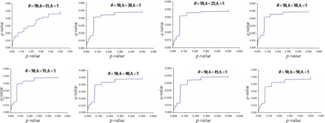
The figure 3 presents another method to identify the variance of 8 multiple tests. By comparing difference of curves from 0 to 0.05 of p-values, the curve has the tendency to go right-bottom. That means the probability of rejecting the null hypotheses descendes proportionally to the difference between sets of DAGs.
Multiple hypothesis testing on Bayesian networks • 1:9
FIGURE 1. Comparison the distribution of p-values obtained in 8 multiple tests on edges of 8 couples of sets of Bayesian networks by histogram. The difference between each couple is varied by three parameters: α: number of edges in the fixed random list for the generation from the initial DAG; ∆: number of random modifications (adding/delecting) of the initial DAG of the first set of BNs to
generate the initial DAG of the second set of BNs; Λ: number of random modifications (adding/delecting) of the initial DAG of to generate the others DAGs in a set of BNs.
FIGURE 2. Comparison the ability of rejecting null hypotheses between 8 multiple tests by varying ∆ - number of random modifications (adding/delecting) of the initial DAG of the first set of BNs to generate the initial DAG of the second set of BNs.
FIGURE 3. Comparison the ability of rejecting null hypotheses between 8 multiple tests by tendency diagram between q-values (cf. Section 2.3.3) and ordered p-values.
6. CONCLUSION
We proposed in this work a new ensemble approach for the comparison of two sets of graph-based models. This approach is based on the multiple test on edges of graph. We described in this paper the solution for dealing with crucial issues causes by the comparison of two sets of Bayesian networks. We also present the quasi essential graph (QEG) that summaries statistically each set of Bayesian networks into a ”most” representative. The main inspiration of this work is the combination of the robustness of the ensemble method and the statistical significance of QEG.
From this point, this approach have to be extended theoretically and experimentally. We want to compare also the directed part of each relationship of nodes (directed edges) and experiment this approach for the real sets of Bayesian networks that are built from a real application.
Acknowledgment
This work was partially supported by a grant from the Pays de la Loire Region (France), Bioinformatics Research Project (BIL).
REFERENCES
Abdi, H. 2007. Bonferroni and sidak corrections for multiple comparisons. Enc. of Meas. and Stat..
Benjamini, Y. and Hochberg, Y. 1995. Controlling the false discovery rate: a practical and powerful approach to multiple testing. Journal of the Royal Statistical Society 57, 1, 125–133.
Chickering, D. 2002. Learning equivalence classes of bayesian-network structure. Journal of Machine Learning Research 2, 445–498.
Dudoit, S., Shaffer, J., and Boldrick, J. 2003. Multiple hypothesis testing in microarray experiments. Statist. Sci. 18, 1, 71–103.
Flesch, I. and Lucas, P. 2007. Markov equivalence in bayesian networks. Advances in Probabilistic Graphical Models, Springer Berlin / Heidelberg 214, 3–38.
Holm, S. 1979. A simple sequentially rejective multiple test procedure. Scandinavian Journal of Statistics 6, 2, 65–70. Koyuturk, M., Szpankowski, W., and Grama, A. 2007. Assessing significance of connectivity and conservation in protein
interaction networks. Journal of Computational Biology 14, 747–764.
Lerner, A., Ogrocki, P., and Thomas, P. 2009. Network graph analysis of category fluency testing. Cognitive and Behavioral Neurology 22, 1, 45–52.
Madigan, D., Andersson, S., Perlman, M., and Volinsky, C. 1996. Bayesian model averaging and model selection for markov equivalence classes of acyclic graphs. Communications in Statistics: Theory and Methods 25, 2493–2519.
Meek, C. 1995. Causal inference and causal explanation with background knowledge. In Proceedings of the Eleventh Conference on Uncertainty in Arti?cial Intelligence, 403–410.
Na¨ım, P., Wuillemin, P.-H., Leray, P., Pourret, O., and Becker, A. 2004. R´eseaux bay´esiens. Eyrolles, Paris.
Pearl, J. and Verma, T. 1991. A theory of inferred causation. In Proceedings of the Second International Conference on Principles of Knowledge Representation and Reasoning, 441–452.
Shefi, O., Golding, I., Segev, R., Ben-Jacob, E., and Ayali, A. 2002. Morphological characterization of in-vitro neuronal networks. Phys. Rev. E. 66, 2.
Westfall, P. and Young, S. 1993. Resampling-based multiple testing: Examples and methods for p-value adjustment. John Wiley and Sons Inc, 10–11.