HAL Id: tel-00578043
https://tel.archives-ouvertes.fr/tel-00578043
Submitted on 18 Mar 2011HAL is a multi-disciplinary open access
archive for the deposit and dissemination of sci-entific research documents, whether they are pub-lished or not. The documents may come from teaching and research institutions in France or abroad, or from public or private research centers.
L’archive ouverte pluridisciplinaire HAL, est destinée au dépôt et à la diffusion de documents scientifiques de niveau recherche, publiés ou non, émanant des établissements d’enseignement et de recherche français ou étrangers, des laboratoires publics ou privés.
Prototypage Rapide et Génération de Code pour DSP
Multi-Coeurs Appliqués à la Couche Physique des
Stations de Base 3GPP LTE
Maxime Pelcat
To cite this version:
Maxime Pelcat. Prototypage Rapide et Génération de Code pour DSP Multi-Coeurs Appliqués à la Couche Physique des Stations de Base 3GPP LTE. Réseaux et télécommunications [cs.NI]. INSA de Rennes, 2010. Français. �NNT : 2010ISAR0011�. �tel-00578043�
Thèse
THESE INSA Rennes
sous le sceau de l’Université européenne de Bretagne pour obtenir le titre de DOCTEUR DE L’INSA DE RENNES Spécialité : Traitement du Signal et des Images
présentée par
Maxime Pelcat
ECOLE DOCTORALE : MATISSE LABORATOIRE : IETRRapid Prototyping and
Dataflow-Based
Code Generation
for the 3GPP LTE
eNodeB Physical Layer
Mapped onto
Multi-Core DSPs
Thèse soutenue le 17.09.2010 devant le jury composé de :
Shuvra BHATTACHARYYA
Professeur à l’Université du Maryland (USA) / Président
Guy GOGNIAT
Professeur des Universités à l’Université de Bretagne Sud / Rapporteur
Christophe JEGO
Professeur des Universités à l’Institut Polytechnique de Bordeaux/ Rapporteur
Sébastien LE NOURS
Maître de conférences à Polytech’ Nantes / Examinateur Slaheddine ARIDHI
Docteur / Encadrant
Jean-François NEZAN
Contents
Acknowledgements 1
1 Introduction 3
1.1 Overview . . . 3
1.2 Contributions of this Thesis . . . 7
1.3 Outline of this Thesis . . . 7
I Background 9 2 3GPP Long Term Evolution 11 2.1 Introduction. . . 11
2.1.1 Evolution and Environment of 3GPP Telecommunication Systems . 11 2.1.2 Terminology and Requirements of LTE. . . 12
2.1.3 Scope and Organization of the LTE Study . . . 14
2.2 From IP Packets to Air Transmission . . . 15
2.2.1 Network Architecture . . . 15
2.2.2 LTE Radio Link Protocol Layers . . . 16
2.2.3 Data Blocks Segmentation and Concatenation. . . 17
2.2.4 MAC Layer Scheduler . . . 18
2.3 Overview of LTE Physical Layer Technologies . . . 18
2.3.1 Signal Air transmission and LTE . . . 18
2.3.2 Selective Channel Equalization . . . 20
2.3.3 eNodeB Physical Layer Data Processing . . . 21
2.3.4 Multicarrier Broadband Technologies and Resources . . . 22
2.3.5 LTE Modulation and Coding Scheme . . . 26
2.3.6 Multiple Antennas . . . 29
2.4 LTE Uplink Features . . . 30
2.4.1 Single Carrier-Frequency Division Multiplexing . . . 30
2.4.2 Uplink Physical Channels . . . 31
2.4.3 Uplink Reference Signals. . . 33
2.4.4 Uplink Multiple Antenna Techniques . . . 34
2.4.5 Random Access Procedure. . . 35
2.5 LTE Downlink Features . . . 37 i
ii CONTENTS
2.5.1 Orthogonal Frequency Division Multiplexing Access . . . 37
2.5.2 Downlink Physical Channels . . . 38
2.5.3 Downlink Reference Signals . . . 40
2.5.4 Downlink Multiple Antenna Techniques . . . 40
2.5.5 UE Synchronization . . . 42
3 Dataflow Model of Computation 45 3.1 Introduction. . . 45
3.1.1 Model of Computation Overview . . . 45
3.1.2 Dataflow Model of Computation Overview. . . 47
3.2 Synchronous Data Flow . . . 50
3.2.1 SDF Schedulability . . . 50
3.2.2 Single Rate SDF . . . 52
3.2.3 Conversion to a Directed Acyclic Graph . . . 53
3.3 Cyclo Static Data Flow . . . 53
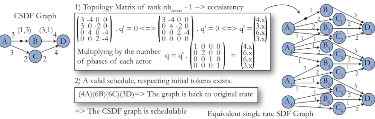
3.3.1 CSDF Schedulability . . . 54
3.4 Dataflow Hierarchical Extensions . . . 54
3.4.1 Parameterized Dataflow Modeling . . . 55
3.4.2 Interface-Based Hierarchical Dataflow . . . 57
4 Rapid Prototyping and Programming Multi-core Architectures 61 4.1 Introduction. . . 61
4.1.1 The Middle-Grain Parallelism Level . . . 61
4.2 Modeling Multi-Core Heterogeneous Architectures . . . 63
4.2.1 Understanding Multi-Core Heterogeneous Real-Time Embedded DSP MPSoC . . . 63
4.2.2 Literature on Architecture Modeling . . . 64
4.3 Multi-core Programming . . . 65
4.3.1 Middle-Grain Parallelization Techniques . . . 65
4.3.2 PREESM Among Multi-core Programming Tools . . . 67
4.4 Multi-core Scheduling . . . 68
4.4.1 Multi-core Scheduling Strategies . . . 68
4.4.2 Scheduling an Application under Constraints . . . 69
4.4.3 Existing Work on Scheduling Heuristics . . . 70
4.5 Generating Multi-core Executable Code . . . 73
4.5.1 Static Multi-core Code Execution. . . 73
4.5.2 Managing Application Variations . . . 74
4.6 Conclusion of the Background Part . . . 74
II Contributions 77 5 A System-Level Architecture Model 79 5.1 Introduction. . . 79
5.1.1 Target Architectures . . . 79
5.1.2 Building a New Architecture Model . . . 82
5.2 The System-Level Architecture Model . . . 83
5.2.1 The S-LAM operators . . . 83
5.2.2 Connecting operators in S-LAM . . . 83
CONTENTS iii
5.2.4 The route model . . . 86
5.3 Transforming the S-LAM model into the route model. . . 88
5.3.1 Overview of the transformation . . . 88
5.3.2 Generating a route step . . . 88
5.3.3 Generating direct routes from the graph model . . . 88
5.3.4 Generating the complete routing table . . . 89
5.4 Simulating a deployment using the route model . . . 90
5.4.1 The message passing route step simulation with contention nodes . . 90
5.4.2 The message passing route step simulation without contention nodes 91 5.4.3 The DMA route step simulation . . . 91
5.4.4 The shared memory route step simulation . . . 91
5.5 Role of S-LAM in the Rapid Prototyping Process . . . 92
5.5.1 Storing an S-LAM Graph . . . 92
5.5.2 Hierarchical S-LAM Descriptions . . . 92
6 Enhanced Rapid Prototyping 95 6.1 Introduction. . . 95
6.1.1 The Multi-Core DSP Programming Constraints . . . 95
6.1.2 Objectives of a Multi-Core Scheduler . . . 96
6.2 A Flexible Rapid Prototyping Process . . . 97
6.2.1 Algorithm Transformations while Rapid Prototyping . . . 97
6.2.2 Scenarios: Separating Algorithm and Architecture . . . 99
6.2.3 Workflows: Flows of Model Transformations. . . 101
6.3 The Structure of the Scalable Multi-Core Scheduler. . . 103
6.3.1 The Problem of Scheduling a DAG on an S-LAM Architecture . . . 104
6.3.2 Separating Heuristics from Benchmarks . . . 104
6.3.3 Proposed ABC Sub-Modules . . . 106
6.3.4 Proposed Actor Assignment Heuristics . . . 107
6.4 Advanced Features in Architecture Benchmark Computers . . . 108
6.4.1 The route model in the AAM process . . . 108
6.4.2 The Infinite Homogeneous ABC . . . 108
6.4.3 Minimizing Latency and Balancing Loads . . . 109
6.5 Scheduling Heuristics in the Framework . . . 111
6.5.1 Assignment Heuristics . . . 112
6.5.2 Ordering Heuristics. . . 113
6.6 Quality Assessment of a Multi-Core Schedule . . . 114
6.6.1 Limits in Algorithm Middle-Grain Parallelism. . . 114
6.6.2 Upper Bound of the Algorithm Speedup . . . 116
6.6.3 Lowest Acceptable Speedup Evaluation . . . 116
6.6.4 Applying Scheduling Quality Assessment to Heterogeneous Target Architectures . . . 117
7 Dataflow LTE Models 119 7.1 Introduction. . . 119
7.1.1 Elements of the Rapid Prototyping Framework . . . 119
7.1.2 SDF4J : A Java Library for Algorithm Graph Transformations . . . 119
7.1.3 Graphiti : A Generic Graph Editor for Editing Architectures, Algo-rithms and Workflows . . . 120
iv CONTENTS
7.1.4 PREESM : A Complete Framework for Hardware and Software
Code-sign . . . 121
7.2 Proposed LTE Models . . . 121
7.2.1 Fixed and Variable eNodeB Parameters . . . 121
7.2.2 A LTE eNodeB Use Case . . . 122
7.2.3 The Different Parts of the LTE Physical Layer Model . . . 124
7.3 Prototyping RACH Preamble Detection . . . 124
7.4 Downlink Prototyping Model . . . 128
7.5 Uplink Prototyping Model . . . 129
7.5.1 PUCCH Decoding . . . 130
7.5.2 PUSCH Decoding . . . 131
8 Generating Code from LTE Models 135 8.1 Introduction. . . 135
8.1.1 Execution Schemes . . . 135
8.1.2 Managing LTE Specificities . . . 137
8.2 Static Code Generation for the RACH-PD algorithm . . . 137
8.2.1 Static Code Generation in the PREESM tool . . . 137
8.2.2 Method employed for the RACH-PD implementation . . . 140
8.3 Adaptive Scheduling of the PUSCH . . . 142
8.3.1 Static and Dynamic Parts of LTE PUSCH Decoding . . . 143
8.3.2 Parameterized Descriptions of the PUSCH. . . 143
8.3.3 A Simplified Model of Target Architectures . . . 145
8.3.4 Adaptive Multi-core Scheduling of the LTE PUSCH . . . 146
8.3.5 Implementation and Experimental Results. . . 149
8.4 PDSCH Model for Adaptive Scheduling . . . 153
8.5 Combination of Three Actor-Level LTE Dataflow Graphs . . . 153
9 Conclusion, Current Status and Future Work 155 9.1 Conclusion . . . 155
9.2 Current Status . . . 156
9.3 Future Work . . . 156
A Available Workflow Nodes in PREESM 159 B French Summary 163 B.1 Introduction. . . 163
B.2 Etat de l’Art . . . 164
B.2.1 Le Standard 3GPP LTE . . . 164
B.2.2 Les Mod`eles Flot de Donn´ees . . . 166
B.2.3 Le Prototypage Rapide et la Programmation des Architectures Mul-ticoeurs . . . 167
B.3 Contributions . . . 169
B.3.1 Un Mod`ele d’Architecture pour le Prototypage Rapide . . . 169
B.3.2 Am´elioration du Prototypage Rapide. . . 171
B.3.3 Mod`eles Flot de Donn´ees du LTE. . . 173
B.3.4 Impl´ementation du LTE `a Partir de Mod`eles Flot de Donn´ees . . . . 173
CONTENTS v
Glossary 189
Personal Publications 191
Acknowledgements
I would like to thank my advisors Dr Slaheddine Aridhi and Pr Jean-Francois Nezan for their help and support during these three years. Slah, thank you for welcoming me at Texas Instruments in Villeneuve Loubet and for spending so many hours on technical discussions, advice and corrections. Jeff, thank you for being so open-minded, for your support and for always seeing the big picture behind the technical details.
I want to thank Pr Guy Gogniat and Pr Christophe Jego for reviewing this thesis. Thanks also to Pr Shuvra S. Bhattacharyya for presiding the jury and to Dr S´ebastien Le Nours for being member of the jury.
It has been a pleasure to work with Matthieu Wipliez and Jonathan Piat. Thank you for your friendship, your constant motivation and for sharing valuable technical insights in computing and electronics. Thanks also to the IETR image and rapid prototyping team for being great co-workers. Thanks to Pr Christophe Moy for his LTE explanations and to Dr Micka¨el Raulet for his help on dataflow. Thanks to Pierrick Menuet for his excellent internship and thanks to Jocelyne Tremier for her administrative support.
This thesis also benefited from many discussions with TIers: special thanks to Eric Biscondi, S´ebastien Tomas, Renaud Keller, Alexandre Romana and Filip Moerman for these. Thanks to the High Performance and Multi-core Processing team for the way you welcomed me to your group.
This thesis benefited from many free or open source tools including Java, Eclipse, JFreeChart, JGraph, SDF4J, LaTeX... Thanks to the open source programmers that participate to the general progress of knowledge.
I am also grateful to Pr Markus Rupp and his team for welcoming me at the Technical University of Vienna and to Pr Olivier D´eforges for supporting this stay. This summer 2009 was both instructive and fun and I thank you for that.
I am thankful to the many chocolate cheesecakes of the Nero caf´e in Truro, Cornwall that were eaten while writing this document: you were delicious.
Many thanks to Dr C´edric Herzet for his help on mathematics and his Belgian fries. Thanks to Karina for reading and correcting this entire document.
Finally, Thanks to my friends, my parents and sister and to St´ephanie for their love and support during these three years.
CHAPTER
1
Introduction
1.1
Overview
The recent evolution of digital communication systems (voice, data and video) has been dramatic. Over the last two decades, low data-rate systems (such as dial-up modems, first and second generation cellular systems, 802.11 Wireless local area networks) have been replaced or augmented by systems capable of data rates of several Mbps, supporting multimedia applications (such as DSL, cable modems, 802.11b/a/g/n wireless local area networks, 3G, WiMax and ultra-wideband personal area networks). One of the latest developments in wireless telecommunications is the 3GPP Long Term Evolution (LTE) standard. LTE enables data rates beyond hundreds of Mbit/s.
As communication systems have evolved, the resulting increase in data rates has ne-cessitated higher system algorithmic complexity. A more complex system requires greater flexibility in order to function with different protocols in diverse environments. In 1965, Moore observed that the density of transistors (number of transistors per square inch) on an integrated circuit doubled every two years. This trend has remained unmodified since then. Until 2003, the processor clock rates followed approximately the same rule. Since 2003, manufacturers have stopped increasing the chip clock rates to limit the chip power dissipation. Increasing clock speed combined with additional on-chip cache memory and more complex instruction sets only provided increasingly faster single-core processors when both clock rate and power dissipation increases were acceptable. The only solution to continue increasing chip performance without increasing power consumption is now to use multi-core chips.
A base station is a terrestrial signal processing center that interfaces a radio access network with the cabled backbone. It is a computing system dedicated to the task of managing user communication. It constitutes a communication entity integrating power supply, interfaces, and so on. A base station is a real-time system because it treats continuous streams of data, the computation of which has hard time constraints. An LTE network uses advanced signal processing features including Orthogonal Frequency Division Multiplexing Access (OFDMA), Single Carrier Frequency Division Multiplexing Access (SC-FDMA), Multiple Input Multiple Output (MIMO). These features greatly increase the available data rates, cell sizes and reliability at a cost of an unprecedented level of processing power. An LTE base station must use powerful embedded hardware platforms.
4 Introduction
Multi-core Digital Signal Processors (DSP) are suitable hardware architectures to execute the complex operations in real-time. They combine cores with processing flexibility and hardware coprocessors that accelerate repetitive processes.
The consequence of evolution of the standards and parallel architectures is an increased need for the system to support multiple standards and multicomponent devices. These two requirements complicate much of the development of telecommunication systems, impos-ing the optimization of device parameters over varyimpos-ing constraints, such as performance, area and power. Achieving this device optimization requires a good understanding of the application complexity and the choice of an appropriate architecture to support this ap-plication. Rapid prototyping consists of studying the design tradeoffs at several stages of the development, including the early stages, when the majority of the hardware and software are not available. The inputs to a rapid prototyping process must then be models of system parts, and are much simpler than in the final implementation. In a perfect design process, programmers would refine the models progressively, heading towards the final implementation.
Imperative languages, and C in particular, are presently the prefered languages to program DSPs. Decades of compilation optimizations have made them a good tradeoff between readability, optimality and modularity. However, imperative languages have been developed to address sequential hardware architectures inspired on the Turing machine and their ability to express algorithm parallelism is limited. Over the years, dataflow languages and models have proven to be efficient representations of parallel algorithms, allowing the simplification of their analysis. In 1978, Ackerman explains the effective-ness of dataflow languages in parallel algorithm descriptions [Ack82]. He emphasizes two important properties of dataflow languages:
data locality: data buffering is kept as local and as reduced as possible,
scheduling constraints reduced to data dependencies: the scheduler that organizes execution has minimal constraints.
The absence of remote data dependency simplifies algorithm analysis and helps to create a dataflow code that is correct-by-construction. The minimal scheduling constraints express the algorithm parallelism maximally. However, good practises in the manipulation of imperative languages to avoid recalculations often go against these two principles. For example, iterations in dataflow redefine the iterated data constantly to avoid sharing a state where imperative languages promote the shared use of registers. But these iterations conceal most of the parallelism in the algorithms that must now be exploited in multi-core DSPs. Parallelism is obtained when functions are clearly separated and Ackerman gives a solution to that: “to manipulate data structures in the same way scalars are manipulated”. Instead of manipulating buffers and pointers, dataflow models manipulate tokens, abstract representations of a data quantum, regardless of its size.
It may be noted that digital signal processing consists of processing streams (or flows) of data. The most natural way to describe a signal processing algorithm is a graph with nodes representing data transformations and edges representing data flowing between the nodes. The extensive use of Matlab Simulink is evidence that a graphically editable plot is suitable input for a rapid prototyping tool.
The 3GPP LTE is the first application prototyped using the Parallel and Real-time Embedded Executives Scheduling Method (PREESM). PREESM is a rapid prototyping tool with code generation capabilities initiated in 2007 and developed during this thesis with the first main objective of studying LTE physical layer. For the development of this
Overview 5
tool, an extensive literature survey yielded much useful research: the work on dataflow process networks from University of California, Berkeley, University of Maryland and Leuven Catholic University, the Algorithm-Architecture Matching (AAM) methodology and SynDEx tool from INRIA Rocquencourt, the multi-core scheduling studies at Hong Kong University of Science and Technology, the dynamic multithreaded algorithms from Massachusetts Institute of Technology among others.
PREESM is a framework of plug-ins rather than a monolithic tool. PREESM is in-tended to prototype an efficient multi-core DSP development chain. One goal of this study is to use LTE as a complex and real use case for PREESM. In 2008, 68% of DSPs shipped worldwide were intended for the wireless sector [KAG+09]. Thus, a multi-core develop-ment chain must efficiently address new wireless application types such as LTE. The term multi-core is used in the broad sense: a base station multi-core system can embed sev-eral interconnected processors of different types, themselves multi-core and heterogeneous. These multi-core systems are becoming more common: even mobile phones are now such distributed systems.
While targeting a classic single-core Von Neumann hardware architecture, it must be noted that all DSP development chains have similar features, as displayed in Figure1.1(a). These features systematically include:
A textual language (C, C++) compiler that generates a sequential assembly code for functions/methods at compile-time. In the DSP world, the generated assembly code is native, i.e. it is specific and optimized for the Instruction Set Architecture (ISA) of the target core.
A linker that gathers assembly code at compile-time in an executable code. A simulator/debugger enabling code inspection.
An Operating System (OS) that launches the processes, each of which comprise several threads. The OS handles the resource shared by the concurrent threads.
Text Editor C Source Code Dedicated Compiler Linker Loader Simulator DSP Core Object Code Executable OS Compiler Options Debugger Software Hardware
(a) A Single-core DSP Development Chain
Editor Algorithm
Description ArchitectureDescription
Generic Compiler CompilerOptions
Linker Loader Simulator DSP Core Object Codes Executables OS Debugger Multicore OS Directives DSP CoreOS ...
(b) A Multi-core DSP Development Chain Figure 1.1: Comparing a Present Single-core Development Chain to a Possible Development Chain for Multi-core DSPs
Incontrast with the DSP world, the generic computing world is currently experiencing an increasing use of bytecode. A bytecode is more generic than native code and is Just-In-Time (JIT) compiled or interpreted at run-time. It enables portability over several ISA
6 Introduction
and OS at the cost of lower execution speed. Examples of JIT compilers are the Java Virtual Machine (JVM) and the Low Level Virtual Machine (LLVM). Embedded systems are dedicated to a single functionality and in such systems, compiled code portability is not advantageous enough to justify performance loss. It is thus unlikely that JIT compilers will appear in DSP systems soon. However, as embedded system designers often have the choice between many hardware configurations, a multi-core development chain must have the capacity to target these hardware configurations at compile-time. As a consequence, a multi-core development chain needs a complete input architecture model instead of a few textual compiler options, such as used in single-core development chains. Extending the structure of Figure 1.1(a), a development chain for multicore DSPs may be imagined with an additional input architecture model (Figure 1.1(b)). This multi-core development chain generates an executable for each core in addition to directives for a multi-core OS managing the different cores at run-time according to the algorithm behavior.
The present multi-core programming methods generally use test-and-refine method-ologies. When processed by hand, parallelism extraction is hard and error-prone, but potentially extremely optimal (depending on the programmer). Programmers of Embed-ded multi-core software will only use a multi-core development chain if:
the development chain is configurable and is compatible with the previous program-ming habits of the individual programmer,
the new skills required to use the development chain are limited and compensated by a proportionate productivity increase,
the development chain eases both design space exploration and parallel software/hard-ware development. Design space exploration is an early stage of system development consisting of testing algorithms on several architectures and making appropriate choices compromising between hardware and software optimisations, based on eval-uated performances.
the exploitation of the automatic parallelism of the development chain produces a nearly optimal result. For example, despite the impressive capabilities of the Texas Instruments TMS320C64x+ compiler, compute-hungry functions are still optimized by writing intrinsics or assembly code. Embedded multi-core development chains will only be adopted when programmers are no longer able to cope with efficient hand-parallelization.
There will always be a tradeoff between system performance and programmabil-ity; between system genericity and optimality. To be used, a development chain must connect with legacy code as well as easing design process. These principles were consid-ered during the development of PREESM. PREESM plug-in functionalities are numerous and combined in graphical workflows that adapt the process to designer goals. PREESM clearly separates algorithm and architecture models to enable design space exploration, introducing an additional input entity named scenario that ensures this separation. The deployment of an algorithm on an architecture is automatic, as is the static code gener-ation and the quality of a deployment is illustrated in a graphical “schedule quality assessment chart”. An important feature of PREESM is that a programmer can debug code on a single-core and then deploy it automatically over several cores with an assured absence of deadlocks.
However, there is a limitation to the compile-time deployment technique. If an al-gorithm is highly variable during its execution, choosing its execution configuration at
Contributions of this Thesis 7
compile-time is likely to bring excessive suboptimality. For the highly variable parts of an algorithm, the equivalent of an OS scheduler for multi-core architectures is thus needed. The resulting adaptive scheduler must be of very low complexity, manage architecture heterogeneity and substantially improve the resulting system quality.
Throughout this thesis, the idea of rapid prototyping and executable code generation is applied to the LTE physical layer algorithms.
1.2
Contributions of this Thesis
The aim of this thesis is to find efficient solutions for LTE deployment over heterogeneous multi-core architectures. For this goal, a fully tested method for rapid prototyping and automatic code generation was developed from dataflow graphs. During the development, it became clear that there was a need for a new input entity or scenario to the rapid prototyping process . The scenario breaks the “Y” shape of the previous rapid prototyping methods and totally separates algorithm from architecture.
Existing architecture models appeared to be unable to describe the target architectures, so a novel architecture model is presented, the System-Level Architecture Model or S-LAM. This architecture model is intended to simplify the high-level view of an architecture as well as to accelerate the deployment.
Mimicing the ability of the SystemC Transaction Level Modeling (TLM) to offer scala-bility in the precision of target architecture simulations, a scalable scheduler was created, enabling tradeoffs between scheduling time and precision. A developper needs to evaluate the quality of a generated schedule and, more precisely, needs to know if the schedule parallelism is limited by the algorithm, by the architecture or by none of them. For this purpose, a literature-based, graphical schedule quality assessment chart is presented. During the deployment of LTE algorithms, it became clear that, for these algorithms, using execution latency as the minimized criterion for scheduling did not produce good load balancing over the cores for the architectures studied. A new scheduling criterion embedding latency and load balancing was developped. This criterion leads to very balanced loads and, in the majority of cases, to an equivalent latency than simply using the latency criterion.
Finally, a study of the LTE physical layer in terms of rapid prototyping and code generation is presented. Some algorithms are too variable for simple compile-time scheduling, so an adaptive scheduler with the capacity to schedule the most dynamic algorithms of LTE at run-time was developed.
1.3
Outline of this Thesis
The outline of this thesis is depicted in Figure 1.2. It is organized around the rapid prototyping and code generation process. After an introduction in Chapter 1, Part I presents elements from the literature used in Part II to create a rapid prototyping method which allows the study of LTE signal processing algorithms. In Chapter2, the 3GPP LTE telecommunication standard is introduced. This chapter focuses on the signal processing features of LTE. In Chapter 3, the dataflow models of computation are explained; these are the models that are used to describe the algorithms in this study. Chapter4 explains the existing techniques for system programming and rapid prototyping.
The S-LAM architecture model developed to feed the rapid prototyping method is presented in Chapter5. In Chapter 6,a scheduler structure is detailed that separates the
8 Introduction
Matching Chapter 3: What is a Dataflow
Model of Computation? state of the art of code parallelization?Chapter 4: What is the
Implementation
Simulation
Chapter 7: How do we model LTE physical layer for execution simulation? Chapter 8: How do we generate code
to execute LTE on multicore DSPs? Chapter 2: How does
LTE work? Rapid prototyping Physical Layer LTE Dataflow MoC Multicore DSP Architecture Model Rapid Prototyping Scenario
Chapter 5: How do we model an architecture? Chapter 6: How do we match? Part I: Background
Part II: Contributions
Figure 1.2: Rapid Prototyping and Thesis Outline
different problems of multi-core scheduling as well as some improvements to the state-of-the-art methods. The two last chapters are dedicated to the study of LTE and the application of all of the previously introduced techniques. Chapter7focuses on LTE rapid prototyping and simulation and Chapter 8 on the code generation. Chapter 8 is divided into two parts; the first dealing with static code generation, and the second with the heart of a multi-core operating system which enables dynamic code behavior: an adaptive scheduler. Chapter 9concludes this study.
Part I
Background
CHAPTER
2
3GPP Long Term Evolution
2.1
Introduction
2.1.1 Evolution and Environment of 3GPP Telecommunication Systems Terrestrial mobile telecommunications started in the early 1980s using various analog systems developed in Japan and Europe. The Global System for Mobile communications (GSM) digital standard was subsequently developed by the European Telecommunications Standards Institute (ETSI) in the early 1990s. Available in 219 countries, GSM belongs to the second generation mobile phone system. It can provide an international mobility to its users by using inter-operator roaming. The success of GSM promoted the creation of the Third Generation Partnership Project (3GPP), a standard-developing organization dedicated to supporting GSM evolution and creating new telecommunication standards, in particular a Third Generation Telecommunication System (3G). The current members of 3GPP are ETSI (Europe), ATIS(USA), ARIB (Japan), TTC (Japan), CCSA (China) and TTA (Korea). In 2010, there are 1.3 million 2G and 3G base stations around the world [gsm10] and the number of GSM users surpasses 3.5 billion [Nor09].
1980 1990 2000 2010 2020 100Mbps 1Mbps 10Mbps 100kbps 10kbps GSM/GPRS/EDGE Narrow band UMTS/HSDPA/HSUPA CDMA OFDMA SC-FDMA
Realistic data rate per user
Number of users 1G 2G 3G 4G Number of users ... GSM UMTSHSPA LTE
Figure 2.1: 3GPP Standard Generations
The existence of multiple vendors and operators, the necessity interoperability when roaming and limited frequency resources justify the use of unified telecommunication stan-dards such as GSM and 3G. Each decade, a new generation of stanstan-dards multiplies the data rate available to its user by ten (Figure2.1). The driving force behind the creation of new standards is the radio spectrum which is an expensive resource shared by many interfering technologies. Spectrum use is coordinated by ITU-R (International Telecommunication
12 3GPP Long Term Evolution
Union, Radio Communication Sector), an international organization which defines tech-nology families and assigns their spectral bands to frequencies that fit the International Mobile Telecommunications (IMT) requirements. 3G systems including LTE are referred to as ITU-R IMT-2000.
Radio access networks must constantly improve to accommodate the tremendous evo-lution of mobile electronic devices and internet services. Thus, 3GPP unceasingly updates its technologies and adds new standards. The goal of new standards is the improvement of key parameters, such as complexity, implementation cost and compatibility, with respect to earlier standards. Universal Mobile Telecommunications System (UMTS) is the first re-lease of the 3G standard. Evolutions of UMTS such as High Speed Packet Access (HSPA), High Speed Packet Access Plus (HSPA+) or 3.5G have been released as standards due to providing increased data rates which enable new mobility internet services like television or high speed web browsing. The 3GPP Long Term Evolution (LTE) is the 3GPP standard released subsequent to HSPA+. It is designed to support the forecasted ten-fold growth of traffic per mobile between 2008 and 2015 [Nor09] and the new dominance of internet data over voice in mobile systems. The LTE standardization process started in 2004 and a new enhancement of LTE named LTE-Advanced is currently being standardized. 2.1.2 Terminology and Requirements of LTE
Cell
Figure 2.2: A three-sectored cell
A LTE terrestrial base station computational center is known as an evolved NodeB or eNodeB, where a NodeB is the name of a UMTS base station. An eNodeB can handle the communication of a few base stations, with each base station covering a geographic zone called a cell. A cell is usually three-sectored with three antennas (or antenna sets) each covering 120° (Figure2.2). The user mobile terminals (commonly mobile phones) are called User Equipment (UE). At any given time, a UE is located in one or more overlapping cells and communicates with a preferred cell; the one with the best air transmission properties. LTE is a duplex system, as communication flows in both directions between UEs and eNodeBs. The radio link between the eNodeB and the UE is called the downlink and the opposite link between UE and its eNodeB is called uplink. These links are asymmetric in data rates because most internet services necessitate a higher data rate for the downlink than for the uplink. Fortunately, it is easier to generate a higher data rate signal in an eNodeB powered by mains than in UE powered by batteries.
In GSM, UMTS and its evolutions, two different technologies are used for voice and data. Voice uses a circuit-switched technology, i.e. a resource is reserved for an active user throughout the entire communication, while data is packet-switched, i.e. data is encapsulated in packets allocated independently. Contrary to these predecessors, LTE is a totally packet-switched network using Internet Protocol (IP) and has no special physical features for voice communication. LTE is required to coexist with existing systems such as UMTS or HSPA in numerous frequency configurations and must be implemented without perturbing the existing networks.
Introduction 13
LTE Radio Access Network advantages compared with previous standards(GSM, UMTS, HSPA...) are [STB09]:
Improved data rates. Downlink peak rate are over 100 Mbit/s assuming 2 UE receive antennas and uplink peak rate over 50Mbit/s. Raw data rates are determined by Bandwidth ∗ Spectral Ef f iciency where the bandwidth (in Hz) is limited by the expensive frequency resource and ITU-R regulation and the spectral efficiency (in bit/s/Hz) is limited by emission power and channel capacity (Section2.3.1). Within this raw data rate, a certain amount is used for control, and so is hidden from the user. In addition to peak data rates, LTE is designed to ensure a high system-level performance, delivering high data rates in real situations with average or poor radio conditions.
A reduced data transmission latency. The two-way delay is under 10 millisecond. A seamless mobility with handover latency below 100 millisecond; handover is the transition when a given UE leaves one LTE cell to enter another one. 100 millisecond has been shown to be the maximal acceptable round trip delay for voice telephony of acceptable quality [STB09].
Reduced cost per bit. This reduction occurs due to an improved spectral effi-ciency; spectrum is an expensive resource. Peak and average spectral efficiencies are defined to be greater than 5 bit/s/Hz and 1.6 bit/s/Hz respectively for the downlink and over 2.5 bit/s/Hz and 0.66 bit/s/Hz respectively for the uplink.
A high spectrum flexibility to allow adaptation to particular constraints of dif-ferent countries and also progressive system evolutions. LTE operating bandwidths range from 1.4 to 20 MHz and operating carrier bands range from 698 MHz to 2.7GHz.
A tolerable mobile terminal power consumption and a very low power idle mode.
A simplified network architecture. LTE comes with the System Architecture Evolution (SAE), an evolution of the complete system, including core network. A good performance for both Voice over IP (VoIP) with small but constant
data rates and packet-based traffic with high but variable data rates.
A spatial flexibility enabling small cells to cover densely populated areas and cells with radii of up to 115 km to cover unpopulated areas.
The support of high velocity UEs with good performance up to 120 km/h and connectivity up to 350 km/h.
The management of up to 200 active-state users per cell of 5 MHz or less and 400 per cell of 10 MHz or more.
Depending on the type of UE (laptop, phone...), a tradeoff is found between data rate and UE memory and power consumption. LTE defines 5 UE categories supporting different LTE features and different data rates.
LTE also supports data broadcast (television for example) with a spectral efficiency over 1 bit/s/Hz. The broadcasted data cannot be handled like the user data because it is sent in real-time and must work in worst channel conditions without packet retransmission.
14 3GPP Long Term Evolution
Both eNodeBs and UEs have emission power limitations in order to limit power con-sumption and protect public health. An outdoor eNodeB has a typical emission power of 40 to 46 dBm (10 to 40 W) depending on the configuration of the cell. An UE with power class 3 is limited to a peak transmission power of 23 dBm (200 mW). The standard allows for path-loss of roughly between 65 and 150 dB. This means that For 5 MHz bandwidth, a UE is able to receive data of power from -100 dBm to -25 dBm (0.1 pW to 3.2 µW). 2.1.3 Scope and Organization of the LTE Study
Channel Coding
eNodeB Downlink Physical Layer Symbol Processing
Channel Decoding Symbol Processing OSI Layer 2
eNodeB Uplink Physical Layer
code
blocks (bits) (complex values)symbols (complex values)symbols
code
blocks (bits) (complex values)symbols (complex values)symbols
OSI Layer 2
Physical Layer Baseband Processing
control link data link IP Packet IP Packet RF RF
Figure 2.3: Scope of the LTE Study
The scope of this study is illustrated in Figure 2.3. It concentrates on the Release 9 LTE physical layer in the eNodeB, i.e. the signal processing part of the LTE stan-dard. 3GPP finalized the LTE Release 9 in December 2009. The physical layer (Open Systems Interconnection (OSI) layer 1) uplink and downlink baseband processing must share the eNodeB digital signal processing resources. The downlink baseband process is itself divided into channel coding that prepares the bit stream for transmission and symbol processing that adapts the signal to the transmission technology. The uplink baseband process performs the corresponding decoding. To explain the interaction with the physical layer, a short description of LTE network and higher layers will be given (in Section2.2). The OSI layer 2 controls the physical layer parameters.
The goal of this study is to address the most computationally demanding use cases of LTE. Consequently, there is a particular focus on the highest bandwidth of 20 MHz for both the downlink and the uplink. An eNodeB can have up to 4 transmit and 4 receive antenna ports while a UE has 1 transmit and up to 2 receive antenna ports. An understanding of the basic physical layer functions assembled and prototyped in the rapid prototyping section is important. For this end, this study considers only the baseband signal processing of the physical layer. For transmission, this means a sequence of complex values z(t) = x(t) + jy(t) used to modulate a carrier in phase and amplitude are generated from binary data and for each antenna port. A single antenna port carries a single complex value s(t) at a one instant in time and can be connected to several antennas.
s(t) = x(t)cos(2πf t) + y(t)sin(2πf t) (2.1) where f is the carrier frequency which ranges from 698 MHz to 2.7GHz. The receiver gets an impaired version of the transmitted signal. The baseband receiver acquires complex values after lowpass filtering and sampling and reconstructing the transmitted data.
An overview of LTE OSI layers 1 and 2 with further details on physical layer technolo-gies and their environment is presented in the following sections. A complete description
From IP Packets to Air Transmission 15
of LTE can be found in [DPSB07], [HT09] and [STB09]. Standard documents describing LTE are available on the web. The UE radio requirements in [36.09a], eNodeBs radio re-quirements in [36.09b], rules for uplink and downlink physical layer in [36.09c] and channel coding in [36.09d] with rules for defining the LTE physical layer.
2.2
From IP Packets to Air Transmission
2.2.1 Network Architecture UE eNodeB eNodeB MME S-GW P-GW Internet eUTRAN = radio terrestrial network EPC = core network X2 S1 S1 HSS PCRF Cell control link data link
Figure 2.4: LTE Systeme Architecture Evolution
LTE introduces a new network architecture named System Architecture Evolution (SAE) and is displayed in Figure2.4where control nodes are grayed compared with data nodes. SAE is divided into two parts:
The Evolved Universal Terrestrial Radio Access Network (E-UTRAN) manages the radio resources and ensures the security of the transmitted data. It is composed entirely of eNodeBs. One eNodeB can manage several cells. Multiple eNodeBs are connected by cabled links called X2 allowing handover management between two close LTE cells. For the case where a handover occurs between two eNodeBs not connected by a X2 link, the procedure uses S1 links and is more complex.
The Evolved Packet Core (EPC) also known as core network, enables packet com-munication with internet. The Serving Gateways (S-GW) and Packet Data Network Gateways (P-GW) ensure data transfers and Quality of Service (QoS) to the mobile UE. The Mobility Management Entities (MME) are scarce in the network. They handle the signaling between UE and EPC, including paging information, UE iden-tity and location, communication security, load balancing. The radio-specific control information is called Access Stratum (AS). The radio-independent link between core network and UE is called Non-Access Stratum (NAS). MMEs delegate the verifica-tion of UE identities and operator subscripverifica-tions to Home Subscriber Servers (HSS). Policy Control and charging Rules Function (PCRF) servers check that the QoS delivered to a UE is compatible with its subscription profile. For example, it can request limitations of the UE data rates because of specific subscription options.
16 3GPP Long Term Evolution
2.2.2 LTE Radio Link Protocol Layers
The information sent over a LTE radio link is divided in two categories: the user-plane which provides data and control information irrespective of LTE technology and the control-plane which gives control and signaling information for the LTE radio link. The protocol layers of LTE are displayed in Figure 2.5 differ between user plane and control plane but the low layers are common to both planes. Figure 2.5associates a unique OSI Reference Model number to each layer. layers 1 and 2 have identical functions in control-plane and user-control-plane even if parameters differ (for instance, the modulation constellation). Layers 1 and 2 are subdivided in:
PDCP RLC MAC PHY PDCP RLC MAC PHY OSI L1 OSI L2 OSI L3 IP tunnel to P-GW IP UE eNodeB IP Packets SAE bearers Radio bearers Logical channels Transport channels Physical channels
(a) User plane
PDCP RLC MAC PHY PDCP RLC MAC PHY RRC RRC
NAS tunnel to MME NAS
UE eNodeB OSI L1 OSI L2 OSI L3 control values SAE bearers Radio bearers Logical channels Transport channels Physical channels (b) Control plane Figure 2.5: Protocol Layers of LTE Radio Link
PDCP layer [36.09h] or layer 2 Packet Data Convergence Protocol is responsible for data ciphering and IP header compression to reduce the IP header overhead. The service provided by PDCP to transfer IP packets is called a radio bearer. A radio bearer is defined as an IP stream corresponding to one service for one UE.
RLC layer [36.09g] or layer 2 Radio Link Control performs the data concatenation and then generates the segmentation of packets from IP-Packets of random sizes which comprise a Transport Block (TB) of size adapted to the radio transfer. The RLC layer also ensures ordered delivery of IP-Packets; Transport Block order can be modified by the radio link. Finally, the RLC layer handles a retransmission scheme of lost data through a first level of Automatic Repeat reQuests (ARQ). RLC manipulates logical channels that provide transfer abstraction services to the upper layer radio bearers. A radio bearer has a priority number and can have Guaranteed Bit Rate (GBR).
MAC layer [36.09f] or layer 2 Medium Access Control commands a low level retrans-mission scheme of lost data named Hybrid Automatic Repeat reQuest (HARQ). The MAC layer also multiplexes the RLC logical channels into HARQ protected trans-port channels for transmission to lower layers. Finally, the MAC layer contains the scheduler (Section2.2.4), which is the primary decision maker for both downlink and uplink radio parameters.
Physical layer [36.09c] or layer 1 comprises all the radio technology required to transmit bits over the LTE radio link. This layer creates physical channels to carry information between eNodeBs and UEs and maps the MAC transport channels to these physical channels. The following sections focus on the physical layer with no distinction drawn between user and control planes.
From IP Packets to Air Transmission 17
Layer 3 differs in control and user planes. Its Control plane handles all information specific to the radio technology, with the MME making the upper layer decisions. The User plane carries IP data from system end to system end (i.e. from UE to P-GW). No further detail will be given on LTE non-physical layers. More information can be found in [DPSB07] p.300 and [STB09] p.51 and 79.
Using both HARQ, employed for frequent and localized transmission errors, and ARQ, which is used for rare but lengthy transmission errors, results in high system reliability while limiting the error correction overhead. The retransmission in LTE is determined by the target service: LTE ensures different Qualities of Service (QoS) depending on the target service. For instance, the maximal LTE-allowed packet error loss rate is 10−2 for conversational voice and 10−6 for transfers based on TCP (Transmission Control Protocol) OSI layer 4. The various QoS imply different service priorities. For the example of a TCP/IP data transfer, the TCP packet retransmission system adds a third error correction system to the two LTE ARQs.
2.2.3 Data Blocks Segmentation and Concatenation
The physical layer manipulates bit sequences called Transport Blocks. In the user plane, many block segmentations and concatenations are processed layer after layer between the original data in IP packets and the data sent over air transmission. Figure2.6summarizes these block operations. Evidently, these operations do not reflect the entire bit transfor-mation process including ciphering, retransmitting, ordering, and so on.
Transport Block (16-149776 bits) CRC(24 bits) Code Block (40-6144 bits) CRC(24 bits)
Rate Matched Block
Turbo Coded Data(120-18432 bits) Treillis termination (12 bits)
Scrambling, Modulation and symbol processing MAC Header MAC SDU
RLC Header RLC PDU RLC SDU
PDCP SDU PDCP Header
Physical Layer
Code Block (40-6144 bits) CRC(24 bits) IP Payload IP Header PDCP SDU PDCP Header IP Payload IP Header RLC SDU RLC Header RLC PDU MAC Layer RLC Layer PDCP Layer
Rate Matching (adaptation to real resources) Turbo Coding with rate 1/3
IP Packet IP Packet
Figure 2.6: Data Blocks Segmentation and Concatenation
In the PDCP layer, the IP header is compressed and a new PDCP header is added to the ciphered Protocol Data Unit (PDU). In the RLC layer, RLC Service Data Units (SDU) are concatenated or segmented into RLC PDUs and a RLC header is added. The MAC layer concatenates RLC PDUs into MAC SDUs and adds a MAC header, forming a Transport Block, the data entity sent by the physical layer. For more details on layer 2 concatenation and segmentation, see [STB09] p.79. The physical layer can carry downlink a Transport Blocks of size up to 149776 bits in one millisecond. This corresponds to a data rate of
18 3GPP Long Term Evolution
149.776M bit/s. The overhead required by layer 2 and upper layers reduces this data rate. Moreover, such a Transport Block is only possible in very favorable transmission conditions with a UE capable of supporting the data rate. Transport Block sizes are determined from radio link adaptation parameters shown in the tables of [36.09e] p.26. An example of link capacity computing is given in Section 7.2.2. In the physical layer, Transport Blocks are segmented into Code Blocks (CB) of size up to 6144 bits. A Code Block is the data unit for a part of the physical layer processing, as will be seen in Chapter 7.
2.2.4 MAC Layer Scheduler
The LTE MAC layer adaptive scheduler is a complex and important part of the eNodeB. It controls the majority of the physical layer parameters; this is the layer that the study will concentrate on in later sections. Control information plays a much greater role in LTE than in the previous 3GPP standards because many allocation choices are concentrated in the eNodeB MAC layer to help the eNodeB make global intelligent tradeoffs in radio access management. The MAC scheduler manages:
the radio resource allocation to each UE and to each radio bearer in the UEs for both downlink and uplink. The downlink allocations are directly sent to the eNodeB physical layer and those of the uplink are sent via downlink control channels to the UE in uplink grant messages. The scheduling can be dynamic (every millisecond) or persistent, for the case of long and predictable services as VoIP.
the link adaptation parameters (Section2.3.5) for both downlink and uplink. the HARQ (Section2.3.5) commands where lost Transport Blocks are retransmitted
with new link adaptation parameters.
the Random Access Procedure (Section 2.4.5) to connect UEs to a eNodeB. the uplink timing alignment (Section2.3.4) to ensure UE messages do not overlap. The MAC scheduler must take data priorities and properties into account before al-locating resources. Scheduling also depends on the data buffering at both eNodeB and UE and on the transmission conditions for the given UE. The scheduling optimizes link performance depending on several metrics, including throughput, delay, spectral efficiency, and fairness between UEs.
2.3
Overview of LTE Physical Layer Technologies
2.3.1 Signal Air transmission and LTE
In [Sha01], C. E. Shannon defines the capacity C of a communication channel impaired by an Additive White Gaussian Noise (AWGN) of power N as:
C = B · log2(1 +
S
N) (2.2)
where C is in bit/s and S is the signal received power. The channel capacity is thus linearly dependent on bandwidth. For the largest possible LTE bandwidth, 20MHz, this corresponds to 133 Mbit/s or 6.65 bit/s/Hz for a S/N = 20dB Signal-to-Noise Ratio or SNR (100 times more signal power than noise) and 8 Mbit/s or 0.4 bit/s/Hz for a -5dB SNR (3 times more noise than signal). Augmenting the transmission power will result in
Overview of LTE Physical Layer Technologies 19
an increased capacity, but this parameter is limited for security and energy consumption reasons. In LTE, the capacity can be doubled by creating two different channels via several antennas at transmitter and receiver sides. This technique is commonly called Multiple Input Multiple Output (MIMO) or spatial multiplexing and is limited by control signaling cost and non-null correlation between channels. It may be noted that the LTE target peak rate of 100Mbit/s or 5 bit/s/Hz is close to the capacity of a single channel. Moreover, the real air tranmission channel is far more complex than its AWGN model. Managing this complexity while maintaining data rates close to the channel capacity is one of the great challenges of LTE deployment.
LTE signals are transmitted from terrestrial base stations using electromagnetic waves propagating at light speed. LTE cells can have a radii of up to 115km, leading to a transmission latency of about 380 µs in both downlink and uplink directions. The actual value of this latency depends on the cell radius and environment. Compensation of this propagation time is performed by UEs and called timing advance ([STB09] p.459).
Path 1 Path 2 Path 3 NLOS Reciprocity H(f) f H(f) f Frequency selective
channel Impulse responsespread in time h(t) t 1 2 3 delay spread h(t) t 1 2 3 delay spread
Figure 2.7: Radio Propagation, Channel Response and Reciprocity Property
Moreover, the signal can undergo several reflections before reaching its target. This effect is known as multiple path propagation and is displayed in Figure2.7. In the time domain, multiple reflections create a Channel Impulse Response (CIR) h(t) with several peaks, each corresponding to a reflection. This effect elongates a received symbol in time and can cause Inter Symbol Interference (ISI) between two successive symbols. The ISI introduces a variable attenuation over the frequency band generating a frequency selective channel. For a given time and a given cell, there are frequency bands highly favorable to data transmission between the eNodeB and a given UE due to its position in space whereas these frequency bands may not be favorable to another UE.
Additional to channel selectivity, the environment parameters that compromise air transmission are fading, noise and interference. In LTE, the frequency reuse factor is 1, i.e. adjacent base stations of a single operator employ the same frequency carrier band. This choice complicates interference handling at cell edges. Ignoring interference, a single air transmission channel is usually modeled with channel convolution and additive noise, which gives in the discrete time domain:
y(n) = h(n) ∗ x(n) + w(n), (2.3)
where n is the discrete time and Ts is the sampling period, x(n) and y(n) are
respec-tively the transmitted and received signals in discrete time, h(n) is the channel impulse response (Figure 2.7) and w(n) is the noise. The equivalent in Fourier discrete domain gives:
20 3GPP Long Term Evolution
Y (k) = H(k)X(k) + W (k), (2.4)
where k is the discrete frequency. In order to estimate H(k), known reference signals (also called pilot signals) are transmitted. A reference signal cannot be received at the same time as the data it is aiding. Certain channel assumptions must be made, including slow modification over time. The time over which a Channel Impulse Response h(t) remains almost constant is called channel coherence time. For a flat Rayleigh fading channel model at 2 GHz, modeling coherence time is about 5 millisecond for a UE speed of 20 km/h ([STB09] p. 576). The faster the UE moves, the faster the channel changes and the smaller the coherence time becomes.
The UE velocity also has an effect on radio propagation, due to the Doppler effect. For a carrier frequency of 2.5 GHz and a UE velocity of 130 km/h, the Doppler effect frequency shifts the signal up to 300 Hz ([STB09] p.478). This frequency shift must be evaluated and compensated for each UE. Moreover, guard frequency bands between UEs are necessary to avoid frequency overlapping and Inter Carrier Interference (ICI).
Figure 2.7 shows a Non-line-of-sight (NLOS) channel, which occurs when the direct path is shadowed. Figure 2.7 also displays the property of channel reciprocity; the channels in downlink and in uplink can be considered to be equal in terms of frequency selectivity within the same frequency band. When downlink and uplink share the same band, channel reciprocity occurs, and so the uplink channel quality can be evaluated from downlink reception study and vice-versa. LTE technologies use channel property estimations H(k) for two purposes:
Channel estimation is used to reconstruct the transmitted signal from the received signal.
Channel sounding is used by the eNodeBs to decide which resource to allocate to each UE. Special resources must be assigned to uplink channel soundings be-cause a large frequency band exceeding UE resources must be sounded initially by each UE to make efficient allocation decisions. The downlink channel sounding is quite straightforward, as the eNodeB sends reference signals over the entire downlink bandwidth.
Radio models describing several possible LTE environments have been developed by 3GPP (SCM and SCME models), ITU-R (IMT models) and a project named IST-WINNER. They offer tradeoffs between complexity and accuracy. Their targeted usage is hardware conformance tests. The models are of two kinds: matrix-based models simulate the propa-gation channel as a linear correlation (equation2.3) while geometry-based models simulate the addition of several propagation paths (Figure2.7) and interferences between users and cells.
LTE is designed to address a variety of environments from mountainous to flat, includ-ing both rural and urban with Macro/Micro and Pico cells. On the other hand, Femtocells with very small radii are planned for deployment in indoor environments such as homes and small businesses. They are linked to the network via a Digital Subscriber Line (DSL) or cable.
2.3.2 Selective Channel Equalization
The air transmission channel attenuates each frequency differently, as seen in Figure 2.7. Equalization at the decoder site consists of compensating for this effect and reconstructing
Overview of LTE Physical Layer Technologies 21
the original signal as much as possible. For this purpose, the decoder must precisely evaluate the channel impulse response. The resulting coherent detection consists of 4 steps:
1. Each transmitting antenna sends a known Reference Signal (RS) using predefined time/frequency/space resources. Additional to their use for channel estimation, RS carry some control signal information. Reference signals are sometimes called pilot signals.
2. The RS is decoded and the H(f ) (Equation 2.4) is computed for the RS time/fre-quency/space resources.
3. H(f ) is interpolated over time and frequency on the entire useful bandwidth. 4. Data is decoded exploiting H(f ).
The LTE uplink and downlink both exploit coherent detection but employ different reference signals. These signals are selected for their capacity to be orthogonal with each other and to be detectable when impaired by Doppler or multipath effect. Orthogonality implies that several different reference signals can be sent by the same resource and still be detectable. This effect is called Code Division Multiplexing (CDM). Reference signals are chosen to have constant amplitude, reducing the transmitted Peak to Average Power Ratio (PAPR [RL06]) and augmenting the transmission power efficiency. Uplink reference signals will be explained in2.4.3and downlink reference signals in 2.5.3.
As the transmitted reference signal Xp(k) is known at transmitter and receiver, it can
be localized and detected. The simplest least square estimation defines:
H(k) = (Y (k) − W (k))/Xp(k) ≈ Y (k)/Xp(k). (2.5)
H(k) can be interpolated for non-RS resources, by considering that channel coherence is high between RS locations. The transmitted data is then reconstructed in the Fourier domain with X(k) = Y (k)/H(k).
2.3.3 eNodeB Physical Layer Data Processing
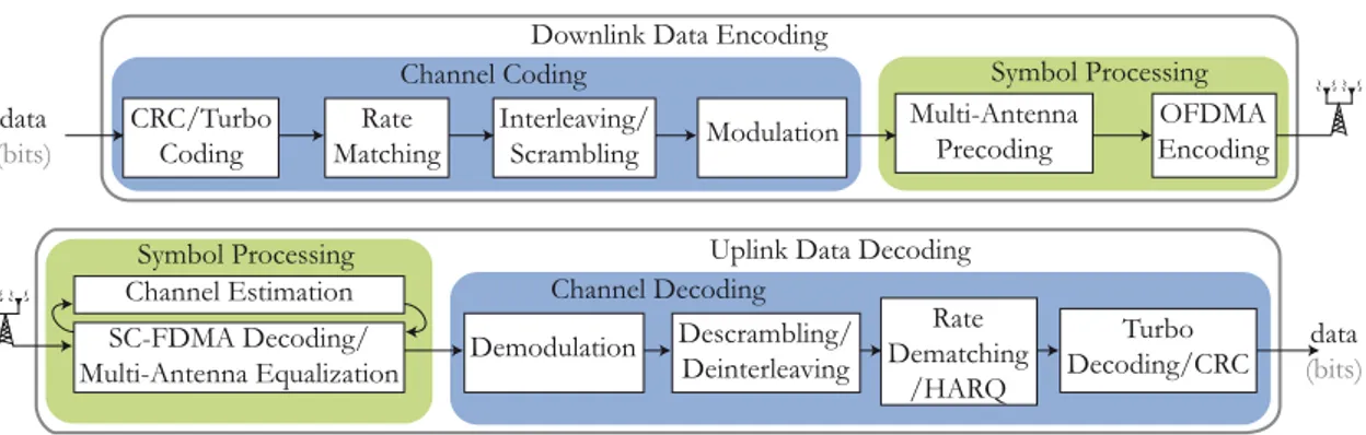
Figure2.8 provides more details of the eNodeB physical layer that was roughly described in Figure2.3. It is still a simplified view of the physical layer that will be explained in the next sections and modeled in Chapter7.
In the downlink data encoding, channel coding (also named link adaptation) prepares the binary information for transmission. It consists in a Cyclic Redundancy Check (CRC) /turbo coding phase that processes Forward Error Correction (FEC), a rate matching phase to introduce the necessary amount of redundancy, a scrambling phase to increase the signal robustness, and a modulation phase that transforms the bits into symbols. The parameters of channel coding are named Modulation and Coding Scheme (MCS). They are detailed in Section 2.3.5. After channel coding, symbol processing prepares the data for transmission over several antennas and subcarriers. The downlink transmission schemes with multiple antennas are explained in Sections2.3.6and2.5.4and the Orthogonal Frequency Division Multiplexing Access (OFDMA), that allocates data to subcarriers, in Section2.3.4.
In the uplink data decoding, the symbol processing consists in decoding Sin-gle Carrier-Frequency Division Multiplexing Access (SC-FDMA) and equalizing signals from the different antennas using channel estimates. SC-FDMA is the uplink broadband
22 3GPP Long Term Evolution
OFDMA Encoding Downlink Data Encoding
data (bits) Multi-Antenna Precoding Modulation Interleaving/ Scrambling Rate Matching CRC/Turbo Coding
Channel Coding Symbol Processing
Turbo Decoding/CRC Uplink Data Decoding
data (bits) Rate Dematching /HARQ Descrambling/ Deinterleaving Channel Decoding Demodulation SC-FDMA Decoding/ Multi-Antenna Equalization Symbol Processing Channel Estimation
Figure 2.8: Uplink and Downlink Data Processing in the LTE eNodeB
transmission technology and is presented in Section 2.3.4. Uplink multiple antenna trans-mission schemes are explained in Section2.4.4. After symbol processing, uplink channel decoding consists of the inverse phases of downlink channel coding because the chosen techniques are equivalent to the ones of downlink. HARQ combining associates the re-peated receptions of a single block to increase robustness in case of transmission errors.
Next sections explain in details these features of the eNodeB physical layer, starting with the broadband technologies.
2.3.4 Multicarrier Broadband Technologies and Resources
LTE uplink and downlink data streams are illustrated in Figure 2.9. The LTE uplink and downlink both employ technologies that enable a two-dimension allocation of resources to UEs in time and frequency. A third dimension in space is added by Multiple Input Multiple Output (MIMO) spatial multiplexing (Section 2.3.6). The eNodeB decides the allocation for both downlink and uplink. The uplink allocation decisions must be sent via the downlink control channels. Both downlink and uplink bands have six possible bandwidths: 1.4, 3, 5, 10, 15, or 20 MHz.
frequency between 1.4
and 20MHz
UE1 UE2 UE3 1 2 3 frequency allocation choices
(a) Downlink: OFDMA
frequency 1 2 3
UE1 UE2 UE3 between 1.4 and 20MHz frequency allocation choices (b) Uplink: SC-FDMA Figure 2.9: LTE downlink and uplink multiplexing technologies
Overview of LTE Physical Layer Technologies 23
Broadband Technologies
The multiple subcarrier broadband technologies used in LTE are illustrated in Figure 2.10. Orthogonal Frequency Division Multiplexing Access (OFDMA) employed for the downlink and Single Carrier-Frequency Division Multiplexing (SC-FDMA) is used for the uplink. Both technologies divide the frequency band into subcarriers separated by 15 kHz (except in the special broadcast case). The subcarriers are orthogonal and data allocation of each of these bands can be controlled separately. The separation of 15 kHz was chosen as a tradeoff between data rate (which increases with the decreasing separation) and protection against subcarrier orthogonality imperfection [R1-05]. This imperfection occurs from the Doppler effect produced by moving UEs and because of non-linearities and frequency drift in power amplifiers and oscillators.
Both technologies are effective in limiting the impact of multi-path propagation on data rate. Moreover, the dividing the spectrum into subcarriers enables simultaneous access to UEs in different frequency bands. However, SC-FDMA is more efficient than OFDMA in terms of Peak to Average Power Ratio (PAPR [RL06]). The lower PAPR lowers the cost of the UE RF transmitter but SC-FDMA cannot support data rates as high as OFDMA in frequency-selective environments. Serial to parallel size M (1200) IFFT size N (2048) 0 0 0 Insert CP size C (144)
Downlink OFDMA Encoding
Freq. Mapping DFT size M (60) IFFT size N (2048) Insert CP size C (144)
Uplink SC-FDMA Encoding
energy time frequency M complex values (1200) to send to U users energy time frequency ... M complex values (60) to send to the eNodeB ... ... ... CP CP ... ... CP CP 1symbol 1symbol M subcar riers M subcar riers 0 0 0 Freq. Mapping 0
Figure 2.10: Comparison of OFDMA and SC-FDMA
Figure 2.10 shows typical transmitter implementations of OFDMA and SC-FDMA using Fourier transforms. SC-FDMA can be interpreted as a linearly precoded OFDMA scheme, in the sense that it has an additional DFT processing preceding the conventional OFDMA processing. The frequency mapping of Figure2.10defines the subcarrier accessed by a given UE.
Downlink symbol processing consists of mapping input values to subcarriers by per-forming an Inverse Fast Fourier Transform (IFFT). Each complex value is then transmitted on a single subcarrier but spread over an entire symbol in time. This transmission scheme protects the signal from Inter Symbol Interference (ISI) due to multipath transmission. It is important to note that without channel coding (i.e. data redundancy and data spreading over several subcarriers), the signal would be vulnerable to frequency selective channels and Inter Carrier Interference (ICI). The numbers in gray (in Figure 2.10) reflect typical parameter values for a signal of bandwidth of 20 MHz. The OFDMA encoding is processed in the eNodeB and the 1200 input values of the case of 20MHz bandwidth carry the data of all the addressed UEs. SC-FDMA consists of a small size Discrete Fourier Transform
24 3GPP Long Term Evolution
(DFT) followed by OFDMA processing. The small size of the DFT is required as this processing is performed within a UE and only uses the data of this UE. For an example of 60 complex values the UE will use 60 subcarriers of the spectrum (subcarriers are shown later to be grouped by 12). As noted before, without channel coding, data would be prone to errors introduced by the wireless channel conditions, especially because of ISI in the SC-FDMA case.
Cyclic Prefix
The Cyclic Prefix (CP) displayed in Figures2.10 and 2.11is used to separate two succes-sive symbols and thus reduces ISI. The CP is copied from the end of the symbol data to an empty time slot reserved before the symbol and protects the received data from timing advance errors; the linear convolution of the data with the channel impulse response is converted into a circular convolution, making it equivalent to a Fourier domain multiplica-tion that can be equalized after a channel estimamultiplica-tion (Secmultiplica-tion 2.3.2). CP length in LTE is 144 samples = 4.8µs (normal CP) or 512 samples = 16.7µs in large cells (extended CP). A longer CP can be used for broadcast when all eNodeBs transfer the same data on the same resources, so introducing a potentially rich multi-path channel. Generally, multipath propagation can be seen to induce channel impulse responses longer than CP. The CP length is a tradeoff between the CP overhead and sufficient ISI cancellation [R1-05].
CP 1 symbol (2048 complex values)
...
160 144 144 144 144 144 144 160
1 slot = 0.5 ms = 7 symbols (with normal CP) = 15360 complex values
Figure 2.11: Cyclic Prefix Insertion
Time Units
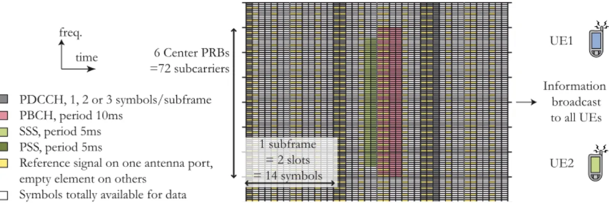
Frequency and timing of data and control transmission is not decided by the UE. The eNodeB controls both uplink and downlink time and frequency allocations. The allocation base unit is a block of 1 millisecond per 180kHz (12 subcarriers). Figure2.12shows 2 PRBs. A PRB carries a variable amount of data depending on channel coding, reference signals, resources reserved for control...
Certain time and frequency base values are defined in the LTE standard, which al-lows devices from different companies to interconnect flawlessly. The LTE time units are displayed in Figure2.12:
A basic time unit lasts Ts = 1/30720000s ≈ 33ns. This is the duration of 1
complex sample in the case of 20 MHz bandwidth. The sampling frequency is thus 30.72M Hz = 8∗3.84M Hz, eight times the sampling frequency of UMTS. The choice was made to simplify the RF chain used commonly for UMTS and LTE. Moreover, as classic OFDMA and SC-FDMA processing uses Fourier transforms, symbols of size power of two enable the use of FFTs and 30.72M Hz = 2048 ∗ 15kHz = 211∗ 15kHz, with 15kHz the size of a subcarrier and 2048 a power of two. Time duration for all other time parameters in LTE is a multiple of Ts.
Overview of LTE Physical Layer Technologies 25
A slot is of length 0.5millisecond = 15360Ts. This is also the time length of a PRB.
A slot contains 7 symbols in normal cyclic prefix case and 6 symbols in extended CP case. A Resource Element (RE) is a little element of 1 subcarrier per one symbol. A subframe lasts 1millisecond = 30720Ts= 2slots. This is the minimum duration
that can be allocated to a user in downlink or uplink. A subframe is also called Transmission Time Interval (TTI) as it is the minimum duration of an independently decodable transmission. A subframe contains 14 symbols with normal cyclic prefix that are indexed from 0 to 13 and are described in the following sections.
A frame lasts 10millisecond = 307200Ts. This corresponds to the time required to
repeat a resource allocation pattern separating uplink and downlink in time in case of Time Division Duplex (TDD) mode. TDD is defined below.
subcarrier spacing 15kHz 1 frame =10ms frequency time 1 PRB 1 slot=0.5ms = 7 symbols 1 subframe=1ms 12 subcarriers 180kHz 1 PRB Bandwidth = between 6 RBs (1.4MHz band) and 100 RBs (20MHz band) 1 RE
Figure 2.12: LTE Time Units
In the LTE standard, the subframe size of 1 millisecond was chosen as a tradeoff between a short subframe which introduces high control overhead and a long subframe which significantly increases the retransmission latency when packets are lost [R1-06b]. Depending on the assigned bandwidth, an LTE cell can have between 6 and 100 resource blocks per slot. In TDD, special subframes protect uplink and downlink signals from ISI by introducing a guard period ([36.09c] p. 9).
Duplex Modes
Figure 2.13 shows the duplex modes available for LTE. Duplex modes define how the downlink and uplink bands are allocated respective to each other. In Frequency Division Duplex (FDD) mode, the uplink and downlink bands are disjoint. The connection is then full duplex and the UE needs to have two distinct Radio Frequency (RF) processing chains for transmission and reception. In Time Division Duplex (TDD) mode, the downlink and the uplink alternatively occupy the same frequency band. The same RF chain can then be used for transmitting and receiving but available resources are halved. In Half-Duplex FDD (HD-FDD) mode, the eNodeB is full duplex but the UE is half-duplex (so can have a single RF chain). In this mode, separate bands are used for the uplink and the downlink but are never simultaneous for a given UE. HD-FDD is already present in GSM.
ITU-R defined 17 FDD and 8 TDD frequency bands shared by LTE and UMTS stan-dards. These bands are located between 698 and 2690 MHz and lead to very different channel behavior depending on carrier frequency. These differences must be accounted for