Prince Edward Island Wind Assessment : Demonstrating the potential of SAR for Sites classification.

(1)

1

Prince Edward Island

Wind Assessment

Demonstrating the potential of SAR for Sites classification

Audrey Lessard Fontaine, Thomas Bergeron, Monique Bernier, Karem Chokmani et Gaétan Lafrance

(2)

(3)

2.5 How many snapshots would be necessary to get a precise picture of the wind s p e e d f r e q u e n c y a n a l y s i s a n d a s s e s s W e i b u l l ' s p a r a m e t e r s ? . . . 5 M e t h o d o l o g y . . . . . . 7 3 . 1 A v a i l a b l e S A R d a t a . . . 7 3 . 2 C o r r e l a t i o n o f f s h o r e - o n s h o r e . . . . . . 8 3 . 3 D i r e c t i o n a l c o m p o s i t e m a p s . . . . . . 1 0 3 . 4 R a n k i n g o f s i t e s . . . . . . t 2 R e s u l t s . . . 1 5 4 . 7 S A R M e t m a s t c o r r e l a t i o n f o r W e i C a n d a t a .. . . . . . 1 5 4 . 2 S A R m e t m a s t c o r r e l a t i o n f o r E n v i r o n m e n t C a n a d a . . . 1 8 4 . 3 D i r e c t i o n a l c o m p o s i t e m a p s . . . . . . 1 8 4 . 4 R a n k i n g o f s i t e s . . . . . . 2 0

(4)

5 D i s c u s s i o n , c o n c l u s i o n a n d re c o m m e n d a t i o n s . . . . . . 2 3 6 A k n o w l e d g e m e n t s . . . . . 2 5 7 B i b l i o g r a p h y . . . . . . 2 7 8 A p p e n d i x . . . . . . 2 9 8 . 1 H o w to o b t a i n b e t t e r r e s u l t s w h e n e x t r a p o l a t i n g s e a m e a s u r e s o n l a n d ? . . . . . . 2 9 9 A p p e n d i x A . . . . . . 3 3 9 . 1 A . 1 H o w to m a k e R o u g h n e s s m a p w i t h GIS : . . . . . . 3 3 9 . 2 A . 2 S t e p s t o m a k e a r o u g h n e s s m a p : . . . . . . 3 3 9.3 A.3 How to use elevation data with digitol elevotion models (DEM)? ... 37 1 0 A p p e n d i x 8 . . . . . . 3 9

1 0 . 1 S i t e s d e s c r i p t i o n s : . . . . . . 3 9 t O . 2 U n v i s i t e d s i t e s . . . . . . 4 8

(5)

1 Introduction

This document is the final report of the first phase of the SAR wind resource assessment for community rinks within the collaboration framework between INRS and WElCan. This report provides the results obtained from a limited dataset of SAR images to demonstrate the potential of SAR images and the type of results obtained from this technique. This project is an application of WESNet Project Number P1.1c - High Resolution Surface Winds Mapping in the Coastal Zone from SAR Satellite lmagery

1 . 1 B a c k g r o u n d

ln 2008 the PEI government initiated a project to support small wind turbine installations of capacity up to 100 kW. Among 25 community rinks interested in the project, five sites have been selected to be funded. For any wind turbine project, the knowledge of wind resources is a critical element of decision making. However, for small wind turbine projects, traditional wind resource assessment programs may appear too expensive. ln addition, the short time frame for executing the complete project, about six months for this particular program, requires a means of quickly assessing and ranking the wind potential at these sites. One of the main goals is to estimate the wind resource at the lowest cost in the shortest period possible.

Under the WESNet group, INRS is pursuing research into the use of Synthetic Aperture Radar (SAR) satellite images of wave patterns for wind resource assessments in marine and coastal areas. Following previous resource assessment projects and data validation, a current project applied to the Magdalene lslands region is giving promising results for determining wind speed distribution and some understanding of the wind direction, in particular specific patterns at given locations for different wind directions. With regards to the criteria previously mentioned, is the SAR approach a good candidate?

To answer this question, an agreement has been made between WElCan and INRS to test the SAR technique for the PEI community rink program. lt is an opportunity to test the applicability of the SAR technique in a real life project as an independent wind assessment method. ln the first phase of collaboration, the SAR technique is tested within certain limits, namely INRS actual SAR images database.

(6)

In the case where INRS and WElCan would choose to extend their collaboration, there would be a second phase of the SAR project where new images might be acquired and be used to compare results with a wind monitoring program for selected sites.

1 . 2 O b j e c t i v e s

The objective of using the SAR approach for PEI community rink project is to: test the

applicability of the SAR technique in a real life as an independent wind assessment technique. To achieve this main objective, three sub-objectives have been determined:

1) To test the correlation between inland and SAR data

2) To create, using only remote sensing data, wind maps of prevalent wind directions 3) To rank the various sites considered with respect to the wind criteria.

1 . 3 P r o i e c t t e a m

L 4 D e l i v e r a b l e s

With regards to the first phase of the project, the deliverables are the present report and a videoconference presentation in order to discuss the SAR techniques, its benefits and limitations, and the results to the partners involved in the PEI Rinks project.

1 . 5 R e p o r t ' s

s t r u c t u r e

The report starts with a review of what the SAR technique is. Then, the methodology employed in this project (chapter 3) and the results (chapter 4) are presented, followed by a conclusion (chapter 5) and three Appendices. Appendix B presented the description of each potential site.

(7)

2 How is it possible to retrieve wind speed from radar satellite

imagery?

2.I First, what is Radar?

A radar is an active instrument emitting and receiving an electromagnetic (EM) signal. In general, the EM signal is linearly polarized and its wavelength may vary from the millimeter to the 102 meter scale. For wind retrieval purposes, radars operating in the Ku, X or C-band are used (between 1.65 and 7.5 cm).

2.2 How a wind map is obtained from a backscatter signal?

The relationship between radar backscatter and wind speed is an indirect one. The radar signal is reflected at the wate/s surface and is influenced by the surface's roughness.

Wind blows over water, modulates the surface. lt creates gravity waves (-m) and capillary waves (-cm) (figure 1). Capillary waves form almost instantaneously and vary rapidly with any change of wind regime

(wind speed or direction). Since their wavelengths are similar, the backscattered signal is mainly related to capillary waves because of Bragg resonant scattering.

Geophysical model function CMODS relates wind speed and direction to signal backscatter (1):

oo = fovoos(0, _{0, Uro)}x PR(0) (1)

Where 0 is the satellite incidence angle, $ the wind direction relative to radar look direction, Uro the wind speed at 10 m and PR is Kirchhoff

polarization ratio.

3

Figure 1 Gravity and Capillary waves on Water surface

(8)

An instantaneous wind map of the region under study is then obtained by inverting the CMOD-S function (see figure 3 as example). By instantaneous, we mean that the wind map obtained represents the wind speed of the whole region at a specific moment in time.

F i g u r e 3 S A R w i n d s p e e d e s t i m a t e f r o m C M O D - 5 fu n c t i o n

2.3 What is the Validity Zone?

The wind map obtained is valid both offshore and up to a few hundred meters from the coastline when using Synthetic Aperture Radar (SAR) imagery. The resolution of such a map is 400m. lf the data use is from a scatterometer, then the resolution is much coarser (-50km) and no data is available close to the coastline. In this specific case study, two satellites were used: SeaWinds Scatterometer aboard QuikSCAT (referred to as QuikSCAT from now on) and RADARSAT-I Synthetic aperture RADAR. They both give the possibility to retrieve wind speeds over a large region through sea surface state analysis. Many studies have demonstrated that wind maps derived from space-borne instruments have a good accuracy level: a small bias and a standard deviation of -1.5 m/s (Bourassa, Legler et al. 2003). Previous work done within the INRS research group even demonstrated that SAR satellites can retrieve wind speeds accurately in complex coastal region (Choisnard, Bernier et al. 2004; Beaucage, Glazer et al. 2007).

2.+ What are the benefits of SAR with respect to met masts?

One of the main benefits of SAR imagery with respect to MET masts is that it allows wind speed estimation over a larger region whereas MET masts only provide local information. Having local information is often problematic because it doesn't give a global picture of the wind distribution over a region. In the wind power industry, wind flow analysis is used to extrapolate the wind information from the nearest MET mast to the site (or region) under study. However, significant

(9)

errors tend to arise from such an extrapolation, especially in complex terrain where wind patterns are very complex (Bowen and Mortensen 1995; Su6rez, Gardiner et al. 1999; Ayotte, Davy et af. 2001; Bechrakis, Deane et al. 2004). Having the opportunity of getting a snopshot of the wind speed distribution over a region gives a better idea of its spatial distribution. When working with numerous snapshots, general trends of wind patterns usually come out, enabling the determination of sub-regions where wind is more favorable. lt is even possible, by comparing the wind maps to the surrounding topographic and roughness maps, to get a better understanding of the surrounding obstacles and of the site's quality with respect to the wind resource aspect.

2.5 How many snapshots

would be necessary

to get a precise picture of

the wind speed frequency analysis and assess Weibull's

parameters?

A simulation work from Pryor et al. established that, using only SAR images, a minimum of 75 images were necessary to estimate accurately (!7oo/o,9 times out of 10) the scale parameter and the mean wind speed of a site, L75 for the shape parameter and 500 images for the power density estimation (Pryor, Nielsen et al. 2004). Work realized here at INRS on the St. Lawrence Gulf region demonstrate that it is possible to obtain a greater accuracy, offshore, by using SAR images in combination with the coarser but more densely sampled QuikSCAT data. The study was done using 80 SAR images and gave promising results (Lessard-Fontaine, Beaucage et al. 2009). As for extrapolation, to determine the precision up to the coastline and inland, further studies are necessary.

(10)

(11)

3 Methodology

3.1 Available SAR data

In the present case, at best, 40 images are covering the region (Figure 4). Since this work is mostly a demonstration of what can be done using satellite imagery, no images were acquired specifically for the study. The SAR images employed for this work were originally intended for another Environment Canada (EC-ISTOP) project, which explains why they are not centered on the region of interest, i.e. PEl. In an ideal situation, allthe images would be centered on Prince Edward lsland, but since it is quicker to buy archived pictures than to acquire new ones, it is not uncommon to have pictures that are imperfectly overlapping and not exactly centered at the desired position. Tools can be developed in order to take into account these issues.

Figure 4 Available SAR lmage density over PE.

With regards with what has been explained in the previous section, having at best 40 images is not sufficient to completely estimate the wind speed distribution and Weibull's parameters. On the other hand, the spatial information in those few images is still very interesting from a qualitative point of view.

(12)

3 . 2 C o r r e l a t i o n

o f f s h o r e - o n s h o r e

Prince Edward island met mast and projected sites

i -I m.Lrnat En !!fmd Ca|r(h Prqdrbr dfin d-dbs mal_me6l l ,br_cdl

fl,**=

0 i 0 2 0 Nrd 63 Utm Z@c 20N Soure l^bran Per Gov Author: Tho|E Ber9€ton Audey{esiard FonlEru

F i g u r e 5 L o c a t l o n o f M E T m a s t , a n d p r o j e c t s a t P E I

To estimate the correlation between offshore and onshore wind for Prince Edward lsland region, the instantaneous offshore wind maps, obtained from the 40 SAR images, were correlated with MET mast data on the island. Two MET mast datasets were used in this research:

Environment Canada 10 m MET masts providing 10 minutes average wind speed and direction every hour. Data has been downloaded from the Environment Canada d a t a b a s e a t t h i s w e b s i t e h t t p : / / c l i m a t e . w e a t h e r o f f i c e . e c . s c . c a l W e l c o m e f . h t m l . T h r e e MET masts were used: North Cape, East point and Saint Peters. They were chosen because of their good SAR image coverage, their location with regard to QuikSCAT data and their proximity to sea,

WElCan MET masts providing 10 minutes average wind speed and direction every 10 minutes. Most of the WElCan MET masts are 10 meters in height, but MET masts of

(13)

Souris, South Lake, Hermanville and East point are at 30m height; they have been brought back to 10m height using the log wind profile formula below for neutral c o n d i t i o n s :

Where V2 is the wind speed at heigh Z2,Vt is the speed already known at height zl and z0 the roughness length, extracted from the roughness maps. For more information about the roughness map, see Appendix A.

To optimize the correlation between SAR and on site data, the MET mast closest to the SAR image time were selected. As mentioned earlier, data obtained from WElCan and Environment Canada are respectively at 10 minutes and one hour intervals. Thus, for the WElCan dataset, data within 5 minutes of the SAR image, were extracted from the database. For the Environment Canada datase! data within 30 minutes of the SAR image was used.

0 tuac,dc,lF. F.c6 USGS @61 P o s i t i o n o f s i n g l e p i x e l ( s t a r s y m b o l ) a n d e x t r a c t i o n

( 2 1

w i n d

(14)

For each met mast, the closest available sea measures were calculated. To insure no inland pixel or pixel influenced by bottom topography was selected NOAA world vector shoreliner was used to create a 1 Km buffer zone along the coast. Two sites were outside the shoreline buffer zone according to the available data: Lennox lsland and North Cape. The NOAA world vector shoreline has a scale of 1:250 000 and has been smoothed in order to create the buffer. Error of precision lies in the local scale and smoothing operation. For those two sites, a two kilometer buffer was used to insure that no inland pixels were taken into account. To look at the Gust wind effect when fast winds are blowing, a 1.2 km*1.2 km (see Figure 6), mean wind speed was also taken around each adjacent site. We correlated both one single pixel and the 1.2 Km *1.2 Km mean wind to MET mast data to verify which one is most accurate.

3 . 3 D i r e c t i o n a l

c o m p o s i t e

m a p s

As mentioned, the data in our possession are not sufficient to provide power density, Weibull statistics and information on power curves for specifics turbines. Nevertheless, SAR data can still provide an initial estimate about which sites are most promising with regards to the wind quality criterion. Two methods were tested to estimate a site quality with respect to other sites, a method called the directional mean wind speed classification, and the other being the directional relative wind speed classification. For both methods, SAR scenes were divided into four subgroups depending on the direction from which the wind was coming: NE if the wind was blowing from an angle between 0 and 90', SE if between 90 and 180', SW if between 180 and 270" and NW if between2TO and 360".

D i r e c t i o n o I n t e o n c I o s s i f i c o t i o n

For this method, all SAR scenes from a same direction were superimposed and the mean wind speed per direction was computed. We then had an average wind speed per direction (NE, SE, S W a n d N W ) fo r t h e w h o l e P r i n c e E d w a r d l s l a n d .

To get a global picture of the wind quality at each site under evaluation, all directions were taken together using a proportional mean of the four directions. First, the SAR pixel closest to site was selected. Note that a 3 km buffer zone was used to insure that no land or high reef pixel was used in the analysis. Then we used QuikSCAT data to determine the proportion of wind along each main direction. The QuikSCAT pixel closest to site was selected and from the 10 years

'

NOAA world vector shorelines were used, see : http://shoreline.noaa.gov/data/datasheets/wvs.html .

(15)

of data available, and used to calculate the proportion of wind respectively from NE, SE, SW and NW. lt is important to note, that QuikSCAT data is only available on the Northern side of the lsland (being available only in open sea). The proportions computed for sites south of the lsland must be analyzed with extra caution. Once, for every site, the proportion of wind from each direction was determined, a proportional mean of the mean wind speed per direction was taken.

D i r e c t i o n a l r e l a t i v e c l a s s i f i c o t i o n

For this second method called, the treatment is almost the same as for the first method except an extra step is added prior to the superposition of scenes from a same direction. This extra step was added in order to work in relative wind speed. We define relative wind speed as being the speed difference between the speed at a specific location and the mean speed of the region at a specific moment. To obtain this relative wind speed, mask a 10 km region around the island was isolated to be analyzed first. The 10 Km zone was chosen because we are only interested in coastal wind pattern in the PEI study case (see the second map of Figure 7). The instantaneous mean wind speed was computed for the coastal region and that value was subtracted from the instantaneous wind map. The map thus obtained is of the local variations of coastal winds (see third map of Figure 7). This give information about the local wind compared to the regional wind for a specific date. lf the wind is weaker at a specific location than in the region, then the relative value will be negative and if it is stronger, the value will be positive. The advantage of working with relative wind speeds compared with true wind speed is to minimize the effect of having images not perfectly centered at the same location.

(16)

)r

v

&"

F i g u r e 7 S t e p s t o w o r k i n r e l a t i v e w i n d s p e e d

The first image at the top is the November l1th 2005 complete scene. A zone of strong winds is observed in the St-Lawrence Gulf, North West of Prince Edward lsland. lf the mean wind speed was taken from this dataset, then it would not be representative of PEI coastal zone since winds in the Gulf are much stronger than around the coast. The middle image shows the data within the buffer zone. For that specific date, the mean wind speed in the buffer zone was of 4.0375 m/s. The third image shows the relative wind speed. Note that the patterns observed are exactly the same in the second and third image, only the scale varies. The fourth image is the composite map of relative wind speed for winds coming from the North-West.

3.4 Ranking of sites

To estimate which sites have the better potential according to our data, we ranked the various sites according to the results of both the directional mean and the directional relative classification. To rank the sites, we used two techniques:

We ranked the sites in order, according to our values, 1 being the sites having best w i n d s .

We divided the sites into five classes of pre-determined wind by dividing the range of results into five equal sub-groups.

1 )

(17)

Once the sites were ranked according to our data, we compared those results to the Canadian wind Atlas. The Atlas is one of the two methods used by WElCan to rank the sites with respect to the wind criterion. We used the same ranking as for our data, except that for the five classes, we used WElCan classes instead of dividing the range of mean wind speed into five equal classes.

(18)

(19)

4 Results

4.1 SAR Met mast correlation for Wei Can data

The correlation has been calculated for each MET mast in comparison with SAR sea measurements (Figure 8). As Figure 8 shows, all MET masts are within a five kilometer range from SAR measurements except Spring Valley which is more than 7 kilometers away.

-4")"t'"""1."-|".""."1..d

Figure 8 Distance between WElcan met mast and SAR sea measurements

8 1 ^ 6 e E 5 ;_{U 4} =

E 3

2 1 0

The correlation observed varied for single pixel versus mean zone. One possible explanation is the variability of wind especially in fast wind conditions and gust. Some MET masts show a better correlation with single pixel other with mean zone. Mean zone tends to attenuate gust effects, but seems to have a greater chance to include pixel biased by bottom topography and reef. Variation is sometime high between the two methods. For example, Lennox lsland has a R2 difference of 0.2852 between the two techniques. Average variation is 0.11 for all sites. Figure 5 shows the best results of both techniques for each site. Since none of the two methods appears to show systematically better correlation, we decide to work with the single pixel technique for the remainder of the study.

Some sites did not show significant correlation. Cape Wolfe (0.1085), Souris (0.1885) and South Lake (0.1838) have very low correlation. The lack of collocated data and the extrapolation of height from L0 to 30m for South Lake and Souris are the main concerns. The distances from

(20)

QuikSCAT data can also be a source of error. The correlation for Lennox lsland (0.5557) and Stanhope (0.9375) appears to be concluding. East point (0.337) and Hermanville (0.3109) also show quite good correlation even if tower heights were at 30 m. Another explanation for low correlation may be the topography. For example, Cape Tryon has a steep cliff of 34m high with 9.7o/o of slope and Cape Wolfe has a 20m one with a slope of 8.4%. Wind change abruptly and can take long distance before attaining a new equilibrium after striking and obstacle of that size.

(21)

11 data 30 u 1{} J 7 data l0 r:l t I. ro 7 0

Sr 0,F tEB i:l.F lo,s

l! ut 10 , ! r F O LJ TE trr o,m u t:t * 5 1 ! J s , * o 14 data zg,fr TI,IF lll,qt t.{xt .l--r:- _{o s l} * G F i g u r e 9 C o r r e l a t i o n l a n d v e r s u s s e a f o r W e i C a n d a t a ( d a t a a r e i n m / s ) 16 data e0,m u.tr * f 1'5,so t.In 0,txt tlr N F = D . Tdata ulJxt l,0.ql t,s ng 10,{xl , il = q3??t

s-i--'

0,m r o r t o 5 data # =t.l!ir7) ID r,o J o l r o L 7

(22)

4 . 2 S A R

m e t m a s t c o r r e l a t i o n fo r E n v i r o n m e n t

C a n a d a

After looking at the previous results, it is important to test if better correlation could be observed with a greater number of collocated data. Some WElCan MET masts don't have long time series and are not always collocated with SAR images.

D ltt 5 o E

E

I

T

t

-Ernolrt

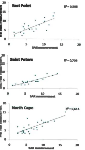
f=051 5 t D t s $InIII 5 t o t s ' o $lrEl o 5 1 0 1 ! t n $lE-i

Figure 10 Correlation of Environment Canada met

mast versus SAR measurements at sea

The comparison done with Environment Canada data were performed on longer time series and contained more comparison points (figure 9). North Cape has 26 co-located data, East Point and Saint-Peters 21 each. Those sites are all very close to sea, North cape is 0.815 Km from the sea, Saint Peters 2.012 Km and East Point 0.115 Km. Roughness is 0.75 for North Cape, 0.01 for Saint-Peters and 0.005 for East Point. High roughness length due to Forest terrain of North Cape can be a source of variations in land/sea data. Topography is smooth for every site, North Cape lies at an altitude of 9m, Saint-Peters at 27m and East Point 7m. Correlation was greater than 0.58 for every site. Those results are in agreements with our hypothesis, larger sets of data conduct to better correlation. lt also shows that extrapolation of speed at different height may induce another bias, East Point is an example. The coastal zone surrounding East Point

$

I'

t E 6 sfthtl| ]=oJs

seems to be subjected to shoal. Obviously, wind is not always orthogonal to coast and is subject to frequent directional variations.

4.3 Directional composite maps

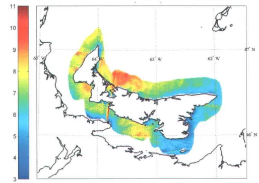
There is a much stronger presence of linear elements and abrupt variations in the composite mean wind speed map (Figure 11) compared to the relative wind speed composite map (see graphic 4 of Figure 7) even though both are of NW direction. These effects, mainly due to the scenes limits varying from one date to another, are smoothed in the relative composite map

n

E-I,

T,

I

o 1 8

(23)

because the data are in relative wind speed and not in true wind speed. Even though, similar global patterns can be observed in both figures, they strike out much more clearly in the relative wind speed map.

Figure 11 Composite mean wind map for winds from NW

Since relative wind speed maps seems to give a clearer picture of PEI wind patterns, let us focus on those (Figure 12). For both winds from North-West and North-East, winds on the southern side of the lsland are much weaker. The North-West composite map also shows a shadow from Tignish to Richmond Bay and stronger wind on the North-East side of the lsland. The map from the South-West shows slightly slower wind around North Cape and on the lsland's North-East side. A higher wind speed zone is also visible around the Richmond Bay, as if the winds were canalized through that Bay. The South-East map is less informative as it contains only one SAR scene; it is thus not really a composite map. Furthermore, the map doesn't cover the entire l s l a n d . T h i s h a s t o b e ta k e n i n t o a c c o u n t i n t h e g l o b a l d a t a a n a l y s i s .

By this visual analysis, we can make the hypothesis that winds on the north shore, east of Richmond Bay, should be best on PEl. On the other hand, winds on the lsland's south-eastern side should be weaker.

(24)

I NdttFwcst i : a ' l r \ 1 i t 2 { { ' \ 1; i \ 1 ,\ 1 6 \ i : I 6J' W .l t r } i .1 i f"

''l

t 6 \ a5 \t 6: \\' I t ( \ 6: \lf F i g u r e 1 2 R e l a t i v e w i n d s p e e d c o m p o s i t e m a p s

+.4 Ranking of sites

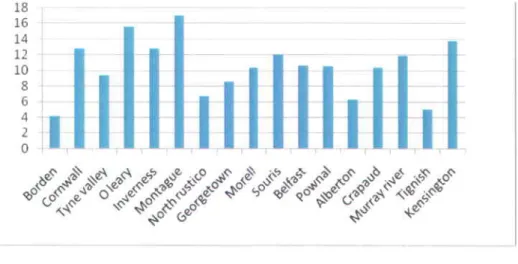
First, it is important to note that some sites are very far from SAR measurements as situated inland. The analysis can be performed forthose sites but accuracy decreases as distance inland increases (see Figure 13). O'leary, Montague and Kensington sites are more than 13 Km away from measurements, adding uncertainties to the results of those sites. Borden, Alberton, North Rustico and Tignish are situated close to the coast: results should be more representative of the real resources, especially the last three located north where QuikSCAT data are also available.

6: \\' t t '

(25)

Figure 13 Distance of projected sites from SAR data

Our results show that sites situated on the North coast of the island have the better potential. North Rustico have the better potentialfollowed by Morell, Inverness, Tignish and Alberton for relative wind speed classification. The south east cities have the lower potential , Pownal, Belfast and Murrray River. Inland cities like Montague, Kensington and O'Leary show medium results, but their distances from the coast make the results less accurate.

Comparison between the mean wind speed, the relative wind speed and the Canadian wind energy Atlas show mitigated results. Data situated south of the island and far inland were particularly under-estimated. Pownal (class 4), Cornwall (class 3)and Kensington (class 4) appear to have been largely underestimated, class of 1 or 2 were attribute instead with the relative and mean wind speed. Distance from shore, distance from the diffusiometer and lack of southern data (7) are main concerns for those results. Alberton, Inverness and Tyne Valley also seem to be far from Canadian wind energy atlas results. Those sites are situated in a close to each other; there might be local phenomenon that modifies wind patterns. The sites in North Rustico and Georgetown have perfect matches between the three techniques. For O'leary, Borden, Belfast, Souris, Morell and Tignish, the Canadian wind atlas data matches with one of the techniques. The relative wind speed techniques match 5 times and the mean zone 4 times. Relative wind speed results seem to be closer than mean method.

(26)

i t ' , : t i L r ; t ' l . i r t t ' r i i l r i l i t , t l ; r l i t i P e r f e c t s i t e s fo r w i n d q u a l i t y are Borden a n d N o r t h R u s t i c o . K e n s i n g t o n , A l b e r t o n , M o r e l l , T i g n i s h a n d P o w n a l f o l l o w a n d a r e in t h e 6.5 to 7 m/s range o f w i n d s p e e d . l t i s i m p o r t a n t t o n o t i c e t h a t R a d a r d a t a a r e e x t r a c t e d f o r a 4 0 0 m p i x e l , a n d C a n a d i a n w i n d e n e r g y w o r k w i t h 4 K m g r i d . R e s u l t s c a n b e v e r y d i f f e r e n t b e c a u s e o n e te c h n i q u e i s a t a m e s o - s c a l e s a n d th e o t h e r a t m i c r o s c a l e s . A l s o , t h e la c k o f d i r e c t i o n a l i n f o r m a t i o n i n t h e N o r t h u m b e r l a n d S t r a i t p o t e n t i a l l y b i a s e d t h e r e s u l t s s o u t h o f t h e i s l a n d . o 1 2 5 2 5

A L , t h o r T h o m a s Bergeron Audrey-Lesserd Fonlarnc

Nad 63 Ulm Zone 20N

S o u r c c C a n a d r a n s p a c e a g e n c y C a n a d r a n w i n d e n e r g y a l l a s C||r! otwind (l-5) J z,s ! Meanwindspeed I Rehtivswindsp€ed Canadian wiod I N R S t i g L t r e 1 4 ( o m p a r i s o n o f p r o J e c t e d s i t e s c l a s s i f r t a t i c ' n n i e t h c i d s

(27)

5 Discussion,

conclusion and recommendations

It is possible to extrapolate data from sea to land, but with certain limitations. There is a 25 to 30 km transition zone at the interface between sea and land where the wind is subject to both sea and land influence (Beaucage, Glazer et al. 2007). The wind on land is thus correlated to the wind at sea in that transition region. Most of Prince Edward lsland lies within the transition zone, thus the onshore wind should be correlated to the offshore wind at some degree. But this correlation is far from being perfect since the wind is highly influenced by upstream obstacles, such as land roughness, topography, etc. (Ricard, Bernier et al. 2005). Extrapolation from land to sea is thus a feasible thing, and is far from being trivial. Results from Environment Canada MET masts show that when the sufficient data is available, correlations are good. Sites situated on the North Coast of the lsland show the best correlations with WElCan data.

The sites chosen by WElCan for the net metering initiative are Alberton, Crapaud Kensington, Murray River and Tignish. From those sites, only Tignish and Alberton have good wind potential, while Murray River received a note of zero for wind quality. For a total of 130 points, wind quality only has a weight of 20 in the total balances. That makes the present study more limited in assessing potential sites for the net metering initiative, but for future study were wind has a stronger weights, it could be more helpful. The GIS technique presented in the appendix can be used to assess wind turbine sitting and obstacles, visibility from the community rink and the area where sound levels exceed the criteria.

This report is a first assessment of what could be done using SAR wind resource assessment. As it has been shown throughout this report, it seems clear that SAR technology has a great potential in helping decision makers in their wind resource analysis, but further developments are needed to better understand the discrepancies between SAR results and the Canadian Wind Atlas. Furthermore, more SAR images would be needed to be able to make a thorough evaluation of the region's potential.

(28)

For a future assessment of wind at Prince Edward lsland the following considerations can be taken into account:

Having a minimum of 40 SAR images dnd a constant density of images throughout the island : That means, acquiring images for the purpose of mapping wind at Prince Edward lsland and subsequently using a SAR approach to derive wind direction, localgradient, fast Fourier transform or wavelet. In that case , directional information would be available all around the island at a Kilometers scale;

Using geostatiscal approach and variogram to know the distances range of validity of sea data;

Taking roughness and topography into account.

(29)

6 Aknowledgements

The authors thank the Prince Edward lsland Energy Corporation for providing the MET mast data, as well as the Wind Energy Institute of Canada for their interest in the project and for providing accommodation in North Cape. They also wish to acknowledge the help of Paul Dockrill, for meaningful discussions and for sharing his time very generously. Finally, thanks to WESNet for fundings.

(30)

(31)

Bibliography

Ayotte, K. W., R. J. Davy, et al. (2001). "A simple temporal and spatial analysis of flow in complex terrain in the context of wind energy modelling." Boundarv-Laver Meteorologv 98(21:275-295. Beaucage, P., A. Glazer, et al. (2OO7l. "Wind assessment in a coastal environment using synthetic aperture radar satellite imagery and a numerical weather prediction model." Canadian Journal of Remote Sensins 33(5): 358-377.

Beaucage, P., M. Bernier, et al. (2008). "Regional Mapping of the Offshore Wind Resource: Towards a Significant Contribution From Space-Borne Synthetic Aperture Radars." leee Journal of Selected Topics in Applied Earth Observations and Remote Sensine 1(1): a8-56.

Bechrakis, D. A., J. P. Deane, et al. (2004). "Wind resource assessment of an area using short term data correlated _{to a long term data set." lglgfE!.gIgy 76(61:725-732.}

Bourassa, M. A., D. M. Legler, et al. (2003). "SeaWinds validation with research vessels." Journal ofGeophvsical Research C: Oceans 108(2): 1-1.

Bowen, A. J. and N. G. Mortensen (1996). "Exploring the limits of the wind atlas analysis and application program." Proceedinss European Wind Energv Conference: 584-587.

Choisnard, J., M. Bernier, et al. (2004). "Mapping of the winds in the Gulf of St. Lawrence using RADARSAT-1 images." Canadian Journal of Remote Sensins 30(a): 504-616.

Lessard-Fontaine, A., P. Beaucage, et al. (2009). Offshore Wind Ressource Assessment Usins Svnthetic Aperture Radar (SAR). AWEA, Chicago.

Manwelf, J.F., J.G McGowan,. and A.L. Rogers (2OO2l, Wind energy exploined-Theory design ond opplication, John Wiley & Sons Ltd, Amherst.

Pryor, S. C., M. Nielsen, et al. (2004). "Can satellite sampling of offshore wind speeds realistically represent wind speed distributions? Part ll: Quantifying uncertainties associated with d i s t r i b u t i o n f i t t i n g m e t h o d s ' . ' @ 4 3 ( 5 ) : 7 3 9 - 7 5 0 .

Ricard, 8., M. Bernier, et al. (2006). "Statistical relations between the measurements of wind in situ and the estimations of winds in a coastal region obtained by the RSO imagery of

RADARSAT-1." 32(2):65-73.

Su6rez, J. C., B. A. Gardiner, et al. (1999). "A comparison of three methods for predicting wind speeds in complex forested terrain." MeteorologicalApplications 6(4l:329342.

(32)

(33)

B

Appendix

8.1 How to obtain better results when extrapolating sea measures on

l a n d ?

A few techniques exist that can improve correlation between land and sea measures. Nevertheless, they were not applied in the present case, because of limited time and resources available for the study. The following techniques could be applied if time and resources were sufficient.

Seporote winds by main directions: (Ricard, Bernier et al. 2005) had separated wind in three class: wind parallel to coast, sea wind and wind coming from land.

Moke o topogrophic clossification _{for eoch site: (Ricard,}Bernier et al. 2006) suggest the following classification: bank, inclination, escarpment and slope. This classification can be possible by making topographic transect on a digital elevation model. To see how it works, fook up the appendix how to retrieve elevotion _{from o digital elevotion}models (DEM). The formula is simple for correctionsS= ZtfACfif, is site height, zd the distance

from shore and s the slope correction. Transect must be in the wind direction. In the case of winds coming from land the transect starts at the site's location.

Correct meosurements with roughness length coefficient: depending on wind directions. The best way to do so is by making a map and transect, the same way as for the DEM. Here are some formulas commonly used:

R o u g l r r t c s s l e r r g t l t : Z = 0 , 5 ' ( H ' 5 / A h )

C o r r c c t i o r r f a c t o r c o r = l n { Z o l Z o 2 i l r r ( h / z O i I l rr (ZolZo _{1 )lrt(h/202)} Wc i ll u I I A(sr tc zo2 _{)= yy..I}5r.t | | A(si tczo 1 )' c o r

(34)

Table 1: Roughness length L 0.9 - 0.6 0.5 0.3 0.2 0 . 1 0.0s 0.03 0.01 5* 10^-3 10^-3 3*10^-4 LO^-4 city forest s u b u r b shelterbelts trees and shrubs close agriculture fields open agriculture fields very open agriculture lands herbs

exposed land snow surfaces sand surfaces water

In the roughness length formula, H is the height, S the cross-section in front of wind, Ah the mean of the horizontal surface of each homogeneous element. Note that tables of roughness length already exist for many specific land uses. For correction factor, zo is turbine height or met mast, ze1 the sea roughness length, zo2 the land sites roughness length. The h in the formula, which is the boundary limit layer, is calculated this way. Within boundary limits layer, wind speed depends on roughness length of terrain and obstacle height.

7 . t

Where X is the distance from the discontinuity and ze' the maximum roughness length between the two sites. lt is important to notice that if the Weibull distribution is not known, correction factor can be applied on raw wind speed.

Roughncss length

Thesric

length teWffienting

the

hedgfrt

(rt wie h winrl his null

stl.d

st$tt ts inEreqse

ltl $

logafitlunic way.. (Trsen et

petersr'tl,

lg8gl

(35)

(') a a () t) t)

(Ricard, Bernier et al. 2006), who worked in the Gasp6sie region, Province of Quebec divided winds in 12 class, 3 for wind regime and 4 for topographic situations of sites. They rejected sites located more than 3 km inland, because of terrestrial wind patterns. They also rejected sites close to river, because of possible effect of canalization of winds in valley. The results obtained for the entire data are shown in Figure 8.

Conrparaison clircctc (R2 = 0,.5227) Suilc i I'c'xtrapolation (R2 = t1,t1266)

20 I t t l 6 1 t l 2 l 0 8 6 4 2 0 0 2 4 6 8 1 0 1 2 1 4 1 6 I [ t 2 0

Vitcssc dc vcnt cstimic par RSO _{d l0 m 1m.s-r})

0 2 4 6 8 r 0 1 2 t 4 t 6 1 8 2 0 Vitcssc dc vcnt cxtrapolcc sur tcrrc (m.s'' )

F i g u r e 1 5 C o m p a r i s o n o f ( R i c a r d , B e r n i e r e t a l . 2 0 0 6 ) d a t a b e f o r e c o r r e c t i o n s ( l e f t ) , a n d a f t e r c o r r e c t i o n s ( r i g h t )

Those results show well the potential of extrapolating SAR offshore estimated wind speed to inshore sites. In the case of Prince Edward lsland, a majority of sites lies in coastal zone and corresponds to good candidate for SAR extrapolation. That situation makes the present study feasible and results show it well. For better results, more constraints have to be taken into account, standard data at L0m and a wider range of scene collections collocated with met mast d a t a . 20 l 8 t 6 I r +

t 2

r 0

8 6 4 2 0 ? a ,a te

_v

t ^l e-Foc

.,tiT.

or

lfF.}{.

'|'

Itrir?^..

-1 ) L

'^ itr

.rgr

^&rl

.trfr

g

3 1

(36)

(37)

9 Appendix A

9 . I A . 1 H o w t o m a k e R o u g h n e s s

m a p w i t h G I S :

Geographic information systems is software made to stock, manage and manipulate geographic information. The three functions of GIS are: Spatial analysis, numerical cartography and database management. Common GIS are Arc GlS, Map info and ldrisi. Some GIS are open sources: Quantum GlS, Grass and others. The software used in the present case is Arc GlS.

9.2 A.2 Steps to make a roughness map:

www.geobase.ca and www.geogratis.ca. Six images were downloaded on the http://scf.rncan.gc.ca. _{The images are part of the project Earth Observotion for} Sustoinoble Development of Forest (EOSD). Landsat images can also be acquired and classified with remote sensing software like PCI Geomatica, Envi and Erdas. Download National Road networks of PEI on Geobase, and the MARITIME STRATEGIC IAND USE DATA BASE (SLUD) on Geogratis. Notice that for more precision you can download topographic data instead of Slud, BNDT or new Canvec 1:50 000 on Geogratis. Layers Batim P and Batim S give you the localization of each building, if you want to work in urban zone or at finer scales.

systems. The projection chose his NAD 83 UTM zone 20N. This projection covers the e n t i r e P r i n c e E d w a r d l s l a n d

analyze.

(38)

I r M d C o Y G r Clatr E l q a d ! o n o 0 . . " I r o e r " " o ' I r o u n . t . r r i r r . o ! r r c o r r s s t a n o I t r c r o u o r e o n g r r c { r t u r e I r a s t " o o " r 2 r t r . - c r o p r r n d I a e , " t . . ! r a a " s . - . " ' . , r . / r o r i e . ! s e r c n - t o . t " t . o r " n o | 2 " " r o " . t , t , , r r t f l o r s n o " , I . " ! a r e c o n i r . . o u ' I r z r o . r r r r o o t " I a r i c o n i r . . o u s - d . n . . r . . , : . ; " , . . ! " " n L i h d ! . : , " " : , , . : " : , - , , " : , . I r o a . v o , o s I e a o r " o " o r . " r I s o s t " u o r " n o I e 2 ! ! r o r d ] . . f - d r n s . I s r s r " u o r" r t I a a a r . o " c t . " r - o l . n

8". -::."""" f;...::,.":""""'""

! o r r c t t . n o - t . r r o [ 2 3 r F i x e d u o o d - o a i s . S a e r " t t . n o - r n . r o E 2 3 2 n r K o F o d - o D . n I r r m t r . n o - n . . 1 ! a " . n , * " 0 * o o - r o . . r . t i g u r e 1 5 C l a s s o l t O 5 D i m a g e s

Reclassification has been done this way :

0 - 1 0 - l l - 1 2 0- No data

20 l- water

30-33 2- exposed

3 l 3- Snow-ice

3 2 4- Rock

34 5 -Urban (different sources)

40-50-51-52 6- Shrub 80-8 1-82-83 7-Wetland 1 0 0 - l l 0 8-grassland t20-t2l 9-Agriculture 200-210-2rt-212-213 lO-Coniferous 220-221-222-223 I 1-Broadleaf 230-231-232-233 l2-Mixedwood l3- Roads F i g u r e 1 6 R e c l a s s i f i c a t i o n o { t h e E O S D i m a g e s 34

(39)

Transform your vector data to raster. Take only the urban zone of The S/ud database and export it to raster, For road networks, make a buffer of 50 m to transform your data from line to polygon, similar to a realistic road width. Most GIS have a Buffer functions. Then convert it to raster. lt's very important to put t h e p i x e l s s i z e a t 1 7 m , t h e s a m e t h a n th e E O S D m a p .

Reclassify the new raster layer, giving a zero to the information and one for no data value. This step will be important, when combining the layers.

Combine your layers. Each layer has to be multiplied with the EOSD layer. Value of zero will represent the top layer value. You have to replace the zero with the corresponding class, 5 for the urban zone, 13 for the road networks, with the reclassify function.

) You now have a nice land use maps. lt's important to save it and conserve it.

F Reclassify for the last time, giving the appropriate roughness length coefficient t o e a c h l a n d u s e c l a s s .

F i g u r e 1 7 R o u g h n e s s l e n g t h s fo r s p e c i f i c l a n d u s e

(40)

) Enjoy your maps and give it nice colors.

Roughness length and land use for Lennox island

I N R S

0 2 250 4 500 9 000 13 500 16 m0 M€lers

Aulhor Thoros Eerg€ron, Audrey+essard Fonlerft Soorce G@base Geogaatrs

) You can do transect easily if your software have a 3D analyst toolbox

Rooehmr. bngh t . , " , f - o w @ u * r " ' I o o r w r ! o r m * r r ! o n w r I O A f oawt*v I ' Lrnd u$ I * . @ c " , * , I " , . I k . l s . c . l * * r ! o , - u * l e s ' x " I 6 e . -I r "o*r l u ' o a [ l l r * , 3 6

(41)

9.3 A.3 How to use elevation data with digital elevation models (DEM)?

DEM are commonly distributed by data providers as open source. There is wide availability of DEM on the internet with different resolution. DEM for all of Canada can be downloaded on Geobase.The United States Geological Survey (USGS) are good providers of DEM. The DEM use in the present case is the Shuttle Radar topography mission (Srtm), which is a NASA platform and can be downloaded on www.USGS.sov. The resolution of DEM is 90m. Some DEM have better resolution but are harder to acquire. The New Aster platform has a resolution of 25m, but data are still hard to acquire and is primarily relevant for sites in the United States. After acquiring the appropriate DEM, it can immediately be used with GIS software.

degrees- if this is attempted, the results of the calculations will be erroneous. UTM or MTM projection is appropriate in that case.

are mostly made for scale of 1:50 000 and higher.

DEM has many applications, in Aeolian industry, it can have the following applications:

Seeing the relief in cross section and viewing the sheltering effects of specific sites. Transects made in the present study are good examples.

Calculating the slope of an environment and applying topographic correction factors on w i n d s .

which it can be viewed can be determined..

(42)

(43)

10 Appendix B

1 0 . 1

S i t e s

d e s c r i p t i o n s

:

Cape Tryon - + F k . d b n o l r . D o s . p h i ( l r N . d 0 ! 5 ! 1 0 : X k e 4 0 5 0 1 0 0 fopograph;c lran!'ecf 1 50 209 250 300

Dislance from shore

3 0 2 8 2E 2 4 t- rg f r e_'14 o € 0 39

(44)

Cape_wolfe r + r i r . { r i o n o t t o p o F h t i r . E N f , C & 1 2 ! : r l l ! : . 4 L r - - r f - r f , r J 30 2 S _ ? 0 . 9 t E T - 1 0 5 0 1 0 0 1 5 0 2 0 0

Distance

from

shore

Topographie lrensecl

(45)

East Point - > D l r i l l o n o l r o P o C q h k r r * * d ? n t 6 fr 21 22 1 8 E , i a D ' -' d r a T " l l 1 C o t n 0 Topographic fr8n$-ecf 0 t ! l r A @ w F r East point 1 0 0 { E n

Distance from shore

(46)

- > ! [ € i l r o n o h o p o r r T h l i i l i n + d Hermanville Hermanville 1 n 2 5 t n E 6 l r c o J -I I U n 0 1 0 0 Topograph;c treos'ecl 2 0 0 3 0 c r 0 0 D i s t a n c e f r o m s h o r e 42

(47)

L e n n o x i s l a n d - } i D [ . d h n o t r o P o m n k ! r r E e d 0 6 ! r S N M s r Lennox island ; 3 0 l 6 2e ; 2 4

u

i 2 0 I _{1 8} i E - 1 6_{' 6} 1 4 ' E ' 1 ? , _{1 0} : E 6 2 : 0 0 5 0 ( Topogrephic fransecf 1 0 0 0 1 5 0 0 2 0 0 0 Distance from shore

(48)

C a 3 l l c S 0 l e n { !

E 0 1 0 0 1 2 0 1 4 0

Dislance from shore

+ > ! l ' e d r o h 0 t r o P . r h r i f i r n + d 2 n tl ' 2 4 2 0 I 1 8 , $ r e o . l { r i -1 0 5 4 ? 0 Iopograpiic tren-cect 44

(49)

South Lake South lake g l0 i& tC ^nr.r. 3 0 2c-2 0 E E l a c -1 0 n 0 Iopographic trersecf 4 5 1 5 0 0

(50)

Spring Valley + o i ' . d b n o t r o P . D h k t ' f f i . d 0 S ! W 2 @ k F r t 50 4 5 4 0 35 E 3 0 EI 'd 25 I 2 A 1 5 1 0 ; 0 1 0 0 0

Profile Graph Subtitl€

2 0 0 0 3 0 0 0 Distance ftom shore

Spring valley

4 6

(51)

? n

I J

r + D l r . d b . o t t o P o 3 4 h k r r * . d

Stanhope

1 000 1 500

Distance fiom shore

0 2 7 5 S r r 6 \ h 20 E E I { E o) -1 0 5 0 0 Topographic harsec! Stanhope 47 2 000

(52)

10.2 Unvisited sites

o fw|f#tr.'|'/'!xct g 000 60 g0 a0 20 t 0 0 0 1 0 0 0 T4,er'Fhtcm'3,cl 2 000 3 000 | 000 Krnrlng[on llurny Rlvrr Nonh c.p. fwt+lticffi# 48

Prince Edward Island Wind Assessment : Demonstrating the potential of SAR for Sites classification.