O
pen
A
rchive
T
OULOUSE
A
rchive
O
uverte (
OATAO
)
OATAO is an open access repository that collects the work of Toulouse researchers and
makes it freely available over the web where possible.
This is an author-deposited version published in :
http://oatao.univ-toulouse.fr/
Eprints ID : 12656
To link to this article : DOI :10.1109/GreenCom-iThings-CPSCom.2013.43
URL :
http://dx.doi.org/10.1109/GreenCom-iThings-CPSCom.2013.43
To cite this version : Tsafack Chetsa, Ghislain Landry and Lefèvre,
Laurent and Pierson, Jean-Marc and Stolf, Patricia and Da Costa,
Georges
A User Friendly Phase Detection Methodology for HPC
Systems' Analysis
. (2013) In: IEEE International Conference on Green
Computing and Communications - GreeCom 2013, 20 August 2013 -
23 August 2013 (Beijing, China).
Any correspondance concerning this service should be sent to the repository
administrator:
[email protected]
A User Friendly Phase Detection Methodology for
HPC Systems’ Analysis
Ghislain Landry Tsafack Chetsa, Laurent Lefevre INRIA, LIP Laboratory (UMR CNRS, ENS, INRIA, UCB)
ENS Lyon, Universit´e de Lyon Lyon, France
Email:{ghislain.landry.tsafack.chetsa, laurent.lefevre}@ens-lyon.fr
Jean-Marc Pierson, Patricia Stolf, Georges Da Costa IRIT (UMR CNRS)
Universit´e de Toulouse Toulouse, France
Email:{pierson, stolf, dacosta}@irit.fr
Abstract—A wide array of today’s high performance com-puting (HPC) applications exhibits recurring behaviours or ex-ecution phases throughout their run-time. Accurate detection of program phases allows reconfiguring the system for a better power/performance trade off; and can reduce the simulation time of programs by identifying regions of code whose performance is critical to the entire program. Program phases are also reflected in different behaviours the system goes through or system phases, which can be used as an alternative means of program phase detection for users lacking expertise. In this paper, we present an execution vector based (EV-based) phase detection, which is an on-line methodology for detecting phases in the behaviour of a HPC system and determining execution points that correspond to these phases. We also present a methodology for defining a small set of EVs representative of the system’s behaviour over a fixed period of time and show that EV-based phase detection identifies recurring phases. Our methodology is illustrated with benchmarks and a real life application.
I. INTRODUCTION
The design of high performance computing (HPC) systems generally places a great emphasis on a handful of components. These include the processor architecture, platform architecture, memory subsystems, communication subsystems, and storage subsystems. The rationale behind this is the need to provide reasonable performance over a wide range of applications. For example, the processor’s architecture is an important factor for compute intensive workloads, so selecting a suitable architecture for the applications task can significantly enhance performance.
A similar analysis can be waged by dimensioning each subsystem. Although this often guarantees acceptable perfor-mance on average over a wide range of applications, it can also result in power dissipation/inefficiency for some workloads or specific execution phases of a workload. e.g., a system designed with a large memory subsystem is likely to dissipate power (as it has to maintain its entire memory subsystem, including the unused part) when running communication in-tensive workloads.
Energy consumption becoming one of the limiting factors in the daily operation of HPC systems, a few research efforts have investigated how to dynamically reconfigure available resources (when executing some workloads or specific phases of a workload) in order to reduce their energy consumption while maintaining acceptable performance [1], [2], [3], [4], [5], [6], [7], [8].
A program phase is without lost of generality a region of execution in which measured program metrics are relatively stable. Roughly speaking, a program’s performance within a phase is relatively stable as well [9]. Consequently, for system adaptation to be effective, it is essential that phase changes be accurately detected; especially, when program phase identification enables reuse of configuration information for reappearing phases.
Detecting program phase changes has been widely ad-dressed in the past [7], [10], [11], [12], [13], [14]. These schemes share a common feature linked to the fact that they either require strong knowledge of the program and/or the system’s architecture or that the program be compiled with specific options or instrumented. Unfortunately, HPC users rarely have adequate skills for performing such tasks. In addition, HPC applications keep growing in complexity and sometimes require experts from multiple domains.
In this paper, we present a runtime user friendly phase detection approach along with a system phase identification methodology and show that it enables identification of recur-ring phases. It is user friendly in the sense that it does not re-quire any knowledge from the users. And differs from previous approaches in that instead of detecting program phase changes we detect system phase changes. As a program phase, a system phase is simply a contiguous interval of execution wherein measured system metrics are relatively stable. Our approach offers the benefits of being independent from any individual programs, easy to use and faster; however, it can also be used for detecting phase changes in a specific workload. Moreover, it also enables detection of system’s idle periods.
The remainder of the paper is organised as follows: In Section II prior work related to program phase changes detection is discussed. Section III details our system phase changes detection mechanism and discusses its effectiveness. Section IV presents the system phase identification technique which goes with system phase changes detection. Finally, Section VI concludes the paper and discusses future work.
II. RELATEDWORK
There is a large body of work dealing with program phase changes detection in the literature. The most popular ap-proaches are based on basic bloc vector, working set signature, and conditional branch counter.
Sherwood et al. [14], [15] and Ratanaworabhan et al. [13] use basic bloc vector (BBVs) to detect program phase changes. A basic bloc vector is a list of all basic blocs entered during program execution, and a count of how many times each basic bloc was run. They keep track of basic bloc vectors at fixed interval and use a similarity threshold afterwards to decide whether a phase change has occurred or not. The Manhattan distance between consecutive basic bloc vectors is used as the similarity criterion. Entire BBVs cannot be stored in hardware, so authors suggested to approximate them by hashing into an accumulator table containing a few large counters.
Balasubramonian et al. [4] use conditional branch counter to detect program phase changes. They keep track of condi-tional branches executed over a fixed execution interval and detect a phase change when the difference in branch counts between consecutive interval exceeds a threshold which varies throughout the program’s execution.
Huang et al. [5] propose to use subroutine as a program phase granularity. They use a hardware call stack to identify major program subroutines and detect program changes by comparing behaviour across different subroutines. Typically, they track the time spent in each subroutine and detect a major phase when the time spent in a subroutine is greater than a given threshold.
Dhodapkar and Smith [16] propose to use program in-struction working set to detect phase changes. They define a program phase as the set of instructions touched in a fixed interval of time and refer to that set as the instruction working set. They next compare consecutive working sets to detect phase changes. However, as for BBVs, complete working sets can be too large to efficiently represent and compare in hardware; to handle this, authors use a loosy-compressed representation of working sets called working set signature [17], [16]. Using the relative signature distance as the similarity metric, phase changes are detected when the relative signature distance between consecutive working set intervals exceeds a predefined threshold.
More recently, Casas et al. [18] have proposed to use signal processing techniques to automatically detect periodic phases in MPI programs. The approach works by analysing the correlation of message passing activity in the application. Karl et al. [19] propose to identify iterative phases in threaded applications through the monitoring and analysis of the control flow graph of the application. Wimmer et al. [20] use trace compilation for phase detection. A program phase change is detected when there is a high trace exit ratio in the created traces. Andreas et al. propose ScarPhase an execution history-based library to detect and classify phases in serial and parallel applications [21].
Our approach is completely different from those listed above. It offers the benefits of being very easy to apply to configurable systems. In addition, it only relies on system information which can potentially allow us to track multiple applications as a single; this is very useful when the system is being optimized for saving energy. For example, on a system running both compute intensive and communication intensive workloads, there is no need to optimize them individually, as optimization made for saving energy considering one ap-plication is likely to degrade performance of the other. The
processor can be slowed down when running communication intensive workloads. Likewise, the network interconnect can be slowed down when running compute intensive workload; thus, considering them individually can result in significant performance degradation.
III. SYSTEMPHASEDETECTION: METHODOLOGY AND
EVALUATION
Program phase detection methods are generally interval-based. During fixed length intervals (also known as the sam-pling interval) specific metrics are measured; the comparison of the current values of the metrics with those from the previous sampling interval determines whether there is a phase change. This means that phase detection methods detect changes in program behaviour that are assumed to result from phase changes. The same assumption holds for system phase changes detection as we show in this paper.
A. Phase Detection
Our phase detection approach works with execution vectors (EVs). As execution vectors go, we define an execution vector as a column vector of sensors including hardware performance counters along with network bytes sent/received and disk read/write counts. Sensors related to hardware performance counters provide insight into the processor and memory ac-tivities, while network and disk related sensors provide infor-mation about network and disk activities respectively. All the sensors are normalized with respect to the number of cycles and only general purpose hardware performance counters are used to avoid redundancy; these hardware performance counters give the following information: the number of retired instructions, last level cache references and misses, and branch instructions and misses.
Unlike work found in the literature, all phases do not necessary have the same length; however, we sample EVs on a per second basis and use the unweighted sliding-average smooth method to reduce white noises. We next define the resemblance or similarity metric between two EVs as the
Manhattan distance between them. The Manhattan distance suits the case since it weighs more heavily differences in each dimension.
A phase change is detected when the Manhattan distance between consecutive EVs exceeds a preset threshold. The threshold is fixed in the sense that it is always the same percentage – we refer to that percentage as the detection
threshold – of the maximum distance between consecutive EVs (e.g., if the detection threshold is X%, then the threshold is X% of the maximum distance between consecutive EVs). However, the maximum distance between consecutive EVs is zeroed once a phase change is detected. So, technically, the threshold varies throughout the system’s life cycle. The maximum existing distance between consecutive EVs is con-tinuously updated until a phase change is detected where it is zeroed. The idea behind zeroing the maximum existing distance when a phase change occurs is to allow detecting phase changes when changing from a phase where distances between consecutive EVs are big to a phase where they are not and vice versa. Algorithm 1 offers a summary of our phase detection algorithm. In a few words, for each newly
sampled EV, Algorithm 1 computes its Manhattan distance to the previously (along the execution time-line) sampled EV and detects a phase change accordingly.
Initialization: threshold = th ; max distance = 0 phase start = False ;
// threshold is a fixed percentage of the maximum existing distance
max_distance while EVs do
Compute dist: the distance between EVt and EVt
−1 and store it
//update the maximum existing distance max_distance
if max distance≤ dist then
max distance← dist
end
if dist≤ max distance ∗ threshold and
phase start is True then Start a new phase phase start = False end
else
if dist > max distance∗ threshold and
phase start is False then phase start = True
//reinitialize the maximum existing distance max distance = 0 end end t + + end
Algorithm 1: EV-based Phase detection algorithm.
B. Phase Detection Results and Analysis
As a case study and proof of concept, we propose to detect phase changes of a two node cluster system running synthetic benchmarks. We next back our proposal with a system running a real life application: the Advance Research Weather Research and Forecasting (WRF-ARW) model [22]. The synthetic benchmarks composed of several benchmarks – including Multi-Grid (MG), Block Tri-diagonal solve (BT), Embarrassingly Parallel (EP), Integer Sort (IS), and Conjugate Gradient (CG) from NPB-3.3 [23] benchmark suite – only differ in that fixed length idle periods are inserted in between workloads in one of them.
Each of the benchmarks composing the synthetic bench-marks has a unique execution pattern, thus using them guaran-tees that the system will go through different behaviours. More importantly, assuming that the execution of a workload in the synthetic benchmark corresponds to an execution phase of the synthetic benchmark, we know in advance when phase changes occur; so doing enables us to tell whether our approach is working or not. In the rest of the paper, we use an empirical evidence based detection threshold of 15%, and a threshold equals to 15% of the maximum existing distance between consecutive EVs, which means that a phase change occurs
when the Manhattan distance between EVtand EVt+1exceeds
15% of the maximum existing distance between consecutive EVs.
We further consider two scenarios, in the first scenario we use a synthetic benchmark which we refer to as bench 1, it successively runs workloads listed above (in the same order, i.e., from left to right starting with MG and ending with CG). The second scenario involves bench 2 which also runs benchmarks listed earlier; it differs from the first scenario in that a 30 second idle period is inserted after each workload. Inserting idle periods in between workloads (bench 2) ensures that successive behaviours through which the system goes are very different, while bench 1 present a more complex scenario where successive behaviours might not differ.
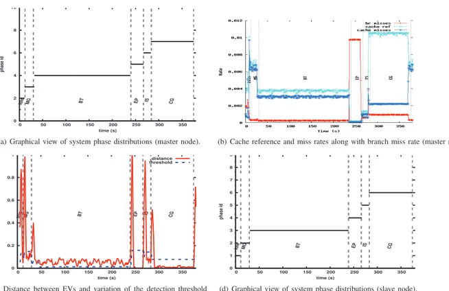
A graphical view of the output of our phase detection algorithm is provided in Figure 1(a) where dashed vertical lines indicate the start and end times of workloads in the synthetic benchmark. The left end of horizontal solid lines indicates the point (in the execution time-line) at which phase changes are detected and their length indicate the duration or length of corresponding phases. The x-axis represents the execution time-line and the y-axis represents IDs associated to detected phases. Note that IDs of phases are non zero integers ordered by their appearance order.
It can be seen from Figure 1(a) that all expected phase changes are detected. Figure 1(c) which shows the variation of distance between consecutive EVs along the execution time-line (x-axis) indicates that micro phases could have been detected when running BT. This is easily achievable depending on the granularity at which one wants to detect phase changes. Indeed, the detection mechanism can use a tighter threshold to detect these regions. As for bench 1, a graphical representation of Algorithm 1 output for bench 2 is given in Figure 2(a) and Figure 2(c). It can be seen that our phase detection approach successfully differentiates periods wherein the system is loaded from those in which it is not. Figure 2(b) and Figure 1(b) corroborate our phase changes detection, as it can be seen that phase changes result in different access pattern to hardware performance counters (not all performance counters are plotted for the sake of clarity). Phases detected on the second node are shown in Figure 1(d) and Figure 2(d).
C. False positives and Sensitivity
Program phase detection generally serves as starting point for power/performance optimization algorithms [1], [2], [3], [4] and simulation. An effective identification of sections of code whose performance is representative of a program can significantly reduce its simulation time [14], [15]. Conse-quently, it is essential that the phase detection mechanism detects phases that actually results in a significant change in the program’s behaviour.
To evaluate our phase detection mechanism we consider three metrics : (i) the sensitivity which is the ability of the phase detection mechanism to detect a change that results in significant change in the system’s behaviour (or performance knowing that performance is relatively stable during a phase). For example, let’s assume that the system has 100 significant behaviour changes. If the phase detection mechanism indicates 87 of these 100 behaviour changes, the sensitivity is 87%. If the phase detection mechanism indicates all of the 100 behaviour changes, then the sensitivity is 100%. “significant behaviour change” being a relative term, we consider a sig-nificant behaviour change as a change of workload from now
0 2 4 6 8 10 0 50 100 150 200 250 300 350 phase id time (s) Idle MG BT EP IS CG
(a) Graphical view of system phase distributions (master node). (b) Cache reference and miss rates along with branch miss rate (master node).
0 0.2 0.4 0.6 0.8 1 0 50 100 150 200 250 300 350 time (s) Idle MG BT EP IS CG distance threshold
(c) Distance between EVs and variation of the detection threshold (master node). 0 1 2 3 4 5 6 7 8 9 0 50 100 150 200 250 300 350 phase id time (s) Idle MG BT EP IS CG
(d) Graphical view of system phase distributions (slave node).
Fig. 1. Phase changes detection using Algorithm 1 when running bench 1; the threshold is 15% of the maximum existing distance between consecutive EVs.
0 2 4 6 8 10 12 0 100 200 300 400 500 phase id time (s)
MG Idle BT Idle EP Idle IS Idle CG
(a) Graphical view of system phase distributions (master node). (b) Cache reference and miss rates along with branch miss rate (master node).
0 0.2 0.4 0.6 0.8 1 0 100 200 300 400 500 time (s)
MG Idle BT Idle EP Idle IS Idle CG
distance threshold
(c) Distance between EVs and variation of the detection threshold (master node.) 0 2 4 6 8 10 0 100 200 300 400 500 phase id time (s)
MG Idle BT Idle EP Idle IS Idle CG
(d) Graphical view of system phase distributions (slave node).
Fig. 2. Phase changes detection using Algorithm 1 when running bench 2; the detection threshold is 15% of the maximum existing distance between consecutive EVs.
TABLE I. PERFORMANCE SUMMARY OF OUR PHASE DETECTION
ALGORITHM CONSIDERING THE TWO SYNTHETIC BENCHMARKS.
Benchmark sensitivity false positives mean detection time
Bench 1 100% 0 0.15 seconds
Bench 2 100% 4 0.5 seconds
on. Notice that the sensitivity will still be 100% if the phase detection mechanism indicates some other phase changes in addition to those initially expected.
Seeking a good sensitivity often leads to false positives; thus, our second evaluation metric is (ii) the number of
false positives. The number of false positive is defined as the number of time where the system’s shows no significant behaviour change but the phase detection technique indicates a phase change. Our third and last evaluation metric (iii) the
mean detection time is the average time the phase detection mechanism takes to notice that a phase change has occurred, i.e., in this case the average time the detection mechanism takes to notice a change of workload.
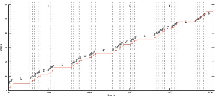
In order to test the effectiveness of our phase detection mechanism, we successively run the synthetic benchmark bench 2 five times and collect statistics related to evaluation metrics listed above. Figure 3 – where steps of the drawn step function indicate detected phases and vertical dashed lines de-limit workloads – gives a graphical representation of the output of our phase detection algorithm when bench 2 is successively run five times. It can be seen that the sensitivity of the phase detection mechanism for that workload is 100%. There is a handful of false positives; however, that is understandable since they occur during idle periods. Despite the assumption that idle periods have a constant behaviour, there might be some system related tasks that are executed during those periods and whose execution can potentially change the system’s behaviour throughout an idle period. Figure 3 also indicates that recurring workloads have the same length according to the phase detection mechanism; this is an interesting property for a phase detection algorithm. Table I summarises evaluation statistics for our synthetic benchmarks. Overall, the mean detection time is less than one second (false positives are not counted).
The mean detection time suggests that the latency of detect-ing a phase is in average less than one second. This is possible because the phase detection software is contained within an independent thread which runs as any other application. The phase detection software nearly has no overhead (so does not need dedicated resources) since it boils down to reading a few sensors and computing the Manhattan distance between EVs.
IV. PHASEREPRESENTATION, SELECTION OF
SIMULATIONPOINTS ANDIDENTIFICATION A. Phase Representation and Selection of Simulation Points
Depending on phases lengths, they can be too large to efficiently represent and compare in hardware, we propose to summarize each phase with only two vectors: the
represen-tative vector and the reference vector. The reference vector of a phase is the closest vector to the centroid of the group of EVs belonging to that phase, whereas the representative vector is the EV resulting from the component wise arithmetic average of all the EVs belonging to the corresponding phase.
The latter (representative vector) can be used in conjunction with selected simulation points to reconstruct the original traces for simulation; however, we do not discuss about trace reconstruction in this paper. As a simulation point goes, we consider as a simulation point for a phase the start point (point at which the first EV occurs) of that phase. The literature suggests selecting simulation points earlier in the execution time-line in order to reduce the time to fast forward (executing the program without performing any cycle accurate simulation) the selected simulation points.
B. Phase Identification
With the need to enable reuse of configuration informa-tion for recurring phases it is essential to accurately iden-tify/recognise recurring phases. We propose to use the ref-erence vector just mentioned earlier for phase identification
and state that two phases P1 and P2 are identified with each
other if the Manhattan distance between them does not exceed a specific percentage of the maximum distance between them. We suggest using the same threshold that was used for phase identification. This is arguable; however, we have good results in practice as illustrated in Figure 4. In Figure 4(a) where there is no idle periods, we nearly identify all the phases in contrary to Figure 4(b). Despite this fact, our phase detection mechanism loosely identifies more than 95% of recurring phases in each scenario. Which is very interesting knowing that the ability to identify recurring phases is a desirable property for phase detection techniques. Recurring phase identification can be used in tuning algorithms to reuse previously found optimal configuration [5], [14], [17]. Notice in passing that none of the idle periods (Figure 4(b)) is identified with any of the workloads.
V. CASESTUDY:THEADVANCERESEARCHWEATHER
RESEARCH ANDFORECASTING(ARW-WRF). Previous sections demonstrate the effectiveness of our phase detection mechanism using synthetic benchmarks. In this section, we investigate its effectiveness using a real life appli-cation representative of HPC workloads: the Advance Research Weather Research and Forecasting (ARW-WRF). WRF-ARW is a fully compressible conservative-form non-hydrostatic at-mospheric model. It uses an explicit time-splitting integration technique to efficiently integrate the Euler equation.
A. Phase detection results for WRF-ARW.
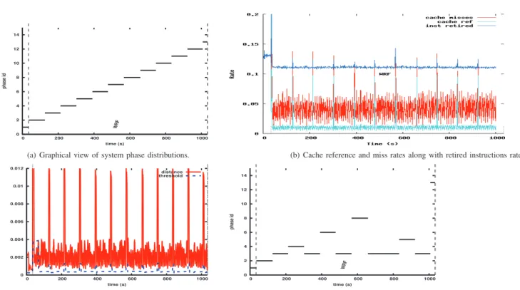
Figure 5 offers a graphical representation of system phases detected using Algorithm 1 when running WRF-AWR. Fig-ure 5(b), where the x-axis represents the execution time-line and the y-axis the access rate of hardware performance counters (not all performance counters are plotted for the sake of clarity), shows without lost of generality WRF-ARW’s re-sources utilization pattern (in terms of performance counters). In using the assumption that (stated earlier in Section III) phase detection methods detect changes in program behaviour that result from phase changes, Figure 5(a) indicates that system phases detected by our algorithm actually correspond to phase changes in the runtime behaviour of WRF-ARW. Note: in Figure 5(a) – where the y-axis represents ids of phases and the x-axis the execution time-line – dashed vertical lines indicate the start and end times of the program and the left
0 10 20 30 40 50 60 0 500 1000 1500 2000 2500 phase id time (s) MGIdle BT Idle EP Idle IS Idle CG IdleMG Idle BT IdleEP Idle IS Idle CG IdleMG Idle BT IdleEP Idle IS Idle CG IdleMG Idle BT IdleEP Idle IS Idle CG IdleMG Idle BT IdleEP Idle IS Idle CG
Fig. 3. Graphical view of phase detected when successively running bench 2 five times. Steps of the drawn step function indicate detected phases. The detection threshold is 15% of the maximum existing distance between consecutive EVs (master node).
0 2 4 6 8 10 12 14 0 200 400 600 800 1000 1200 1400 1600 1800 phase id time (s) MG BT EP IS CG MG BT EP IS CG MG BT EP IS CG MG BT EP IS CG MG BT EP IS CG
(a) Graphical view of system phase distributions resulting from five successive executions of bench 1 (master node).
0 2 4 6 8 10 12 14 0 500 1000 1500 2000 2500 phase id time (s)
MG Idle BT Idle EP IdleISIdle CG Idle MG Idle BT Idle EP IdleISIdle CG Idle MG Idle BT Idle EP IdleISIdle CG Idle MG Idle BT Idle EP IdleISIdle CG Idle MG Idle BT Idle EP IdleISIdle CG
(b) Graphical view of system phase distributions resulting from five successive executions of bench 2 (master node).
Fig. 4. Phase identification illustrated with five successive run of each benchmark; the detection threshold is 15% . Phases are compared using reference vectors instead of the representative vectors.
end of horizontal solid lines indicates the point at which phase changes are detected.
Figure 5(d) and Figure 5(a) are alike except that in Fig-ure 5(d), phases identified with each other are on the same horizontal solid line (some consecutive phases are merged). Overall, it can be seen that our phase detection algorithm performs as well with ”home made” synthetic benchmarks as with a real life workload. The sensitivity is 100% and there isn’t any false positive (Phase changes in the program runtime behaviour Figure 5(b) are detected as phase changes by the phase detection mechanism.). However, phase changes detec-tion may be influenced by the detecdetec-tion threshold. Figure 6
offers a graphical representation of the output of the phase detection mechanism using a 10% detection threshold. Note that one of the phases previously detected using using a 15% detection threshold (with the same algorithm) in now broken into two phases. The next section analysis the influence of the detection threshold on phase changes detection.
B. Impact of the Detection Threshold on phase detection
The selection of the detection threshold basically depends on the granularity at which one would like to detect phase changes. Table II shows how the number of phases detected varies with respect to the detection threshold when the system
0 2 4 6 8 10 12 14 0 200 400 600 800 1000 phase id time (s) WRF
(a) Graphical view of system phase distributions. (b) Cache reference and miss rates along with retired instructions rate.
0 0.002 0.004 0.006 0.008 0.01 0.012 0 200 400 600 800 1000 time (s) distance threshold
(c) Distance between EVs and variation of the detection threshold
0 2 4 6 8 10 12 14 0 200 400 600 800 1000 phase id time (s) WRF
(d) Graphical representation of system phase distributions: phases identified as similar to each other are on the same horizontal line
Fig. 5. Phase changes detection using Algorithm 1 when running WRF-AWR; the detection threshold is 15% of the maximum existing distance between consecutive EVs.
was running WRF-ARW. The number of phases detected is one when the whole application is considered as a single phase. Table II indicates that when the detection threshold is too low nearly no execution vector is similar to another. Likewise when the detection threshold is too high all the execution vectors are similar to each other.
TABLE II. VARIATION OF THE NUMBER OF PHASES DETECTED WITH
RESPECT TO THE DETECTION THRESHOLD.
Detection threshold (%) 1 5 10 15 20 30 35 40 50
Number of phases detected 1 2 13 12 27 52 1 1 1
0 2 4 6 8 10 12 14 0 200 400 600 800 1000 phase id time (s) WRF
Fig. 6. Phase changes detection using Algorithm 1 when running WRF-AWR; the detection threshold is 10% of the maximum existing distance between consecutive EVs.
VI. CONCLUSIONS ANDFUTUREDIRECTIONS
In this paper, we have presented an on-line system phase detection methodology, which is an alternative to program phase detection. It takes advantage of the fact that program phases are also reflected in the behaviour of the system through resource utilisation to detect phases of the system instead of those of individual applications. System resource utilisation related information gathered in execution vectors are transmitted to the phase detection mechanism which detects phase changes using a similarity metric. We use our phase detection mechanism to detect phases of a system running two synthetic benchmarks and a real life application. We carried out experiments to demonstrate its effectiveness considering three evaluation metrics the sensitivity, the number of false positives, and the mean detection time. Those metrics, revealed the ability of our phase detection mechanism to capture program phases including idle periods at the system level.
We further presented a methodology for representing a fixed runtime period of the system with a small set of execution vectors and selecting execution points. We also introduce the concept of reference vector which serves in place of the representative vector for both on-line and off-line phase identification.
As our phase detection mechanism does not require any information about applications being executed, it can be used to address the energy consumption problem of a wide array of applications by users lacking good knowledge of their applica-tions. Although, this work effort is originally destined to power
oriented research [24] (can be easily used for characterizing workloads in order to apply power reduction schemes with nearly no overhead) , we believe it can be used in several aspects of computer architecture. We presented results for a two node system; however, the methodology is adapted to HPC systems as it is applied to individual nodes of the system regardless of others. The same workload often have different behaviours on some nodes among those it is running on, our methodology allows making power reduction decisions locally to the node. Future directions include evaluating our phase detection mechanism in detecting phases of more real-life workloads and introducing a threshold selection procedure.
ACKNOWLEDGMENT
This work is supported by the INRIA large scale initia-tive Hemera (http://www.grid5000.fr). focused on “develop-ing large scale parallel and distributed experiments”. Some experiments of this article were performed on the Grid5000 platform (http://www.grid5000.fr) an initiative from the French Ministry of Research through the ACI GRID incentive action, INRIA, CNRS and RENATER and other contributing partners (http://www.grid5000.fr).
REFERENCES
[1] M. Y. Lim, V. W. Freeh, and D. K. Lowenthal, “Adaptive, trans-parent frequency and voltage scaling of communication phases in mpi programs,” in Proceedings of the 2006 ACM/IEEE conference on
Supercomputing, SC ’06, (New York, NY, USA), ACM, 2006. [2] H. Kimura, T. Imada, and M. Sato, “Runtime energy adaptation with
low-impact instrumented code in a power-scalable cluster system,” in
Proceedings of the 2010 10th IEEE/ACM International Conference on Cluster, Cloud and Grid Computing, CCGRID ’10, (Washington, DC, USA), pp. 378–387, IEEE Computer Society, 2010.
[3] G. L. Tsafack, L. Lefevre, J.-M. Pierson, P. Stolf, and G. Da Costa, “Beyond cpu frequency scaling for a fine-grained energy control of hpc systems,” in SBAC-PAD 2012 : 24th International Symposium on
Computer Architecture and High Performance Computing, (New York City, USA), pp. 132–138, IEEE, oct 2012.
[4] R. Balasubramonian, D. Albonesi, A. Buyuktosunoglu, and S. Dwarkadas, “Memory hierarchy reconfiguration for energy and performance in general-purpose processor architectures,” in
Proceedings of the 33rd annual ACM/IEEE international symposium on Microarchitecture, MICRO 33, (New York, NY, USA), pp. 245–257, ACM, 2000.
[5] M. C. Huang, J. Renau, and J. Torrellas, “Positional adaptation of processors: application to energy reduction,” in Proceedings of the 30th
annual international symposium on Computer architecture, ISCA ’03, (New York, NY, USA), pp. 157–168, ACM, 2003.
[6] A. Buyuktosunoglu, T. Karkhanis, D. H. Albonesi, and P. Bose, “Energy efficient co-adaptive instruction fetch and issue,” in Proceedings of the
30th annual international symposium on Computer architecture, ISCA ’03, (New York, NY, USA), pp. 147–156, ACM, 2003.
[7] R. I. Bahar and S. Manne, “Power and energy reduction via pipeline balancing,” in Proceedings of the 28th annual international symposium
on Computer architecture, ISCA ’01, (New York, NY, USA), pp. 218– 229, ACM, 2001.
[8] M. Huang, J. Renau, S.-M. Yoo, and J. Torrellas, “A framework for dynamic energy efficiency and temperature management,” in
Pro-ceedings of the 33rd annual ACM/IEEE international symposium on Microarchitecture, MICRO 33, (New York, NY, USA), pp. 202–213, ACM, 2000.
[9] T. Sherwood, Calder, and B. Calder, “Time varying behavior of pro-grams,” tech. rep., 1999.
[10] M. Otte and S. Richardson, “An hmm applied to semi-online program phase analysis,” Technical Report CU-CS-1034-07, University of Col-orado at Boulder, 2007.
[11] C. Ding, S. Dwarkadas, M. C. Huang, K. Shen, and J. B. Carter, “Program phase detection and exploitation,” in Proceedings of the
20th international conference on Parallel and distributed processing, IPDPS’06, (Washington, DC, USA), pp. 279–279, IEEE Computer Society, 2006.
[12] V. Bala, E. Duesterwald, and S. Banerjia, “Dynamo: a transparent dynamic optimization system,” in PLDI’00, pp. 1–12, 2000. [13] P. Ratanaworabhan and M. Burtscher, “Program phase detection based
on critical basic block transitions,” in Proceedings of the ISPASS 2008
- IEEE International Symposium on Performance Analysis of Systems and software, ISPASS ’08, (Washington, DC, USA), pp. 11–21, IEEE Computer Society, 2008.
[14] T. Sherwood, S. Sair, and B. Calder, “Phase tracking and prediction,” in
Proceedings of the 30th annual international symposium on Computer architecture, ISCA ’03, (New York, NY, USA), pp. 336–349, ACM, 2003.
[15] T. Sherwood, E. Perelman, and B. Calder, “Basic block distribution analysis to find periodic behavior and simulation points in applications,” in Proceedings of the 2001 International Conference on Parallel
Ar-chitectures and Compilation Techniques, PACT ’01, (Washington, DC, USA), pp. 3–14, IEEE Computer Society, 2001.
[16] A. S. Dhodapkar and J. E. Smith, “Managing multi-configuration hardware via dynamic working set analysis,” in Proceedings of the 29th
annual international symposium on Computer architecture, ISCA ’02, (Washington, DC, USA), pp. 233–244, IEEE Computer Society, 2002. [17] A. S. Dhodapkar and J. E. Smith, “Dynamic microarchitecture adap-tation via co-designed virtual machines,” in Intl. Solid-State Circuits
Conference, Digest of Technical Papers, ISSCC ’02, (Washington, DC, USA), pp. 198–199, IEEE Computer Society, 2002.
[18] M. Casas, R. M. Badia, J. Labarta, C. Bischof, M. Bcker, P. Gibbon, G. R. Joubert, B. Mohr, F. P. (eds, M. Casas, R. M. Badia, and J. Labarta, “Automatic phase detection of mpi applications,” in In:
Proceedings of the 14th Conference on Parallel Computing (ParCo 2007), Aachen and Juelich, 2007.
[19] K. F¨urlinger and S. Moore, “Detection and analysis of iterative behavior in parallel applications,” in ICCS (3) (M. Bubak, G. D. van Albada, J. Dongarra, and P. M. A. Sloot, eds.), vol. 5103 of Lecture Notes in
Computer Science, pp. 261–267, Springer, 2008.
[20] C. Wimmer, M. S. Cintra, M. Bebenita, M. Chang, A. Gal, and M. Franz, “Phase detection using trace compilation,” in PPPJ (B. Stephenson and C. W. Probst, eds.), pp. 172–181, ACM, 2009. [21] A. Sembrant, D. Black-Schaffer, and E. Hagersten, “Phase behavior in
serial and parallel applications,” in IISWC, pp. 47–58, IEEE Computer Society, 2012.
[22] W. C. Skamarock, J. B. Klemp, J. Dudhia, D. O. Gill, D. M. Barker, W. Wang, and J. G. Powers, “A description of the advanced research WRF version 2,” NCAR Tech Note, vol. NCAR/TN-468+STR, 2005. [23] NASA, “Nas parallel benchmarks.”
http://www.nas.nasa.gov/publications/npb.html, Jan. 2013.
[24] G. L. Tsafack, L. Lefevre, and P. Stolf, “A three step blind approach for improving hpc systems’ energy performance,” in EE-LSDS 2013
: Energy Efficiency in Large Scale Distributed Systems conference, (Vienna, Austria), Springer, april 2013.