L'interprétation de la sélection d'habitat comme mécanisme de coexistence chez une communauté de sciuridé via le comportement d'approvisionnement
70
0
0
Texte intégral
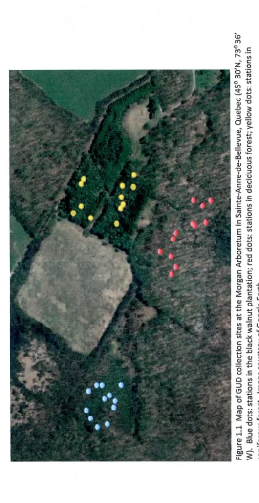
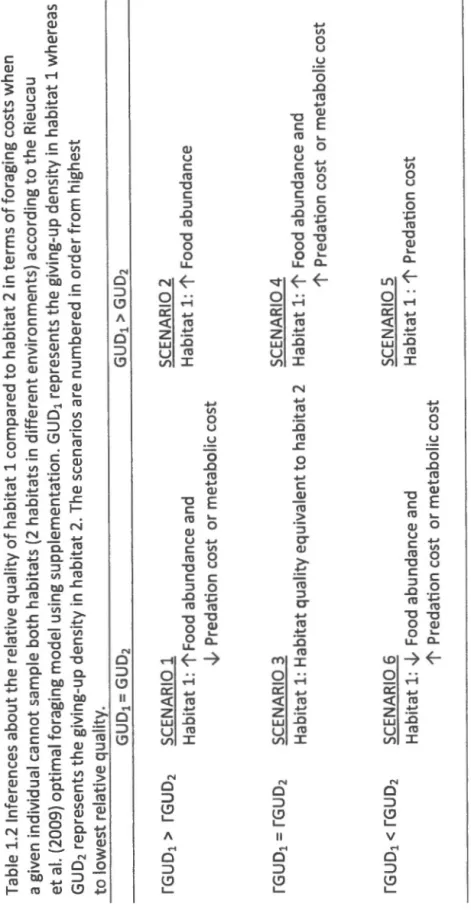
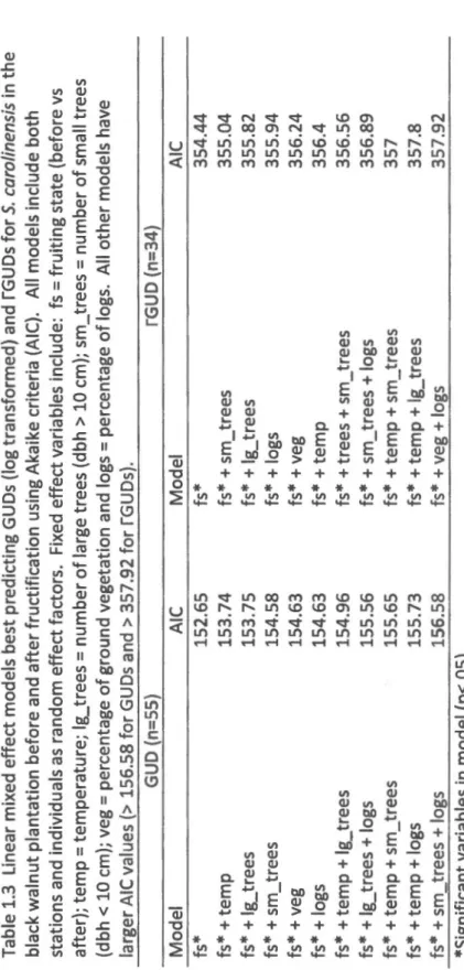
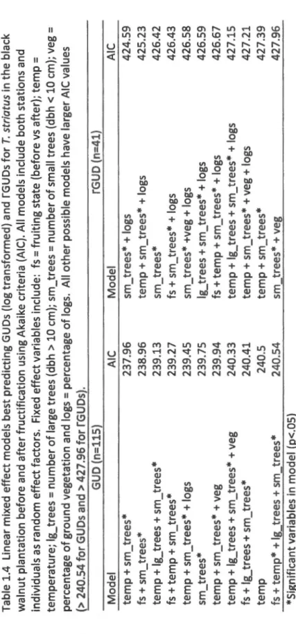
Figure


+7


Documents relatifs