End-to-end latency and temporal consistency analysis in networked real-time systems

O

pen

A

rchive

T

OULOUSE

A

rchive

O

uverte (

OATAO

)

OATAO is an open access repository that collects the work of Toulouse researchers and

makes it freely available over the web where possible.

This is an author-deposited version published in :

http://oatao.univ-toulouse.fr/

Eprints ID : 13243

To link to this article :

DOI:10.1504/IJCCBS.2014.064667

URL :

http://dx.doi.org/10.1504/IJCCBS.2014.064667

To cite this version :

Lauer, Michael and Boniol, Frédéric and Pagetti, Claire

and Ermont, Jérôme End-to-end latency and temporal consistency analysis in

networked real-time systems. (2014) International Journal of Critical

Computer-Based Systems, vol. 5 (n° 3/4). pp. 172-196. ISSN 1757-8779

Any correspondance concerning this service should be sent to the repository

administrator:

staff-oatao@listes-diff.inp-toulouse.fr

End-to-end latency and temporal consistency

analysis in networked real-time systems

Micha

¨

el Lauer*

Université de Toulouse,

7, avenue du Colonel Roche BP 54200, 31031 Toulouse Cedex 4, France E-mail: michael.lauer@laas.fr *Corresponding author

Fr

´

ed

eric Boniol and Claire Pagetti

´

2, avenue Edouard Belin BP 4025, F31055 Toulouse, France E-mail: frederic.boniol@onera.fr E-mail: claire.pagetti@onera.fr

J

er

´

ome Ermont

ˆ

Abstract: Critical embedded systems are often designed as a set of real-time

tasks, running on shared computing modules, and communicating through networks. Because of their critical nature, such systems have to meet strict timing properties. To help the designers to prove the correctness of their system, the real-time systems community has developed numerous approaches for analysing the worst case scenarios either on the processors (e.g., worst case response time of a task) or on the networks (e.g., worst case traversal time of a message). These approaches provide results only for local components behaviours. However, there is a growing need for having a global view of the system, in order to determine end-to-end properties. Such a property applies to functional chains which describe the behaviour of sequences of tasks. We propose an approach to analyse worst case behaviour along functional chains in critical embedded systems. It is based on mixed integer linear programming (MILP) and is general in the sense that it can be applied to a variety of end-to-end properties. This paper focuses on two essential properties: end-to-end latency and temporal consistency. This work was supported by the French National Research Agency within the SATRIMMAP project.

Keywords: real-time systems; embedded systems; worst-case analysis;

Reference to this paper should be made as follows: Lauer, M., Boniol, F.,

Pagetti, C. and Ermont, J. (2014) ‘End-to-end latency and temporal consistency analysis in networked real-time systems’, Int. J. Critical

Computer-Based Systems, Vol. 5, Nos. 3/4, pp.172–196.

Biographical notes: Micha¨el Lauer received his PhD in Networks, Telecommunications, Systems and Architecture at the University of Toulouse. He is an Associate Professor in the Dependable Computing and Fault Tolerance group at the Laboratory for Analysis and Architecture of Systems (LAAS-CNRS) in Toulouse and he teaches at the University of Toulouse. His research interests include issues related to the verification of real-time requirements in critical embedded systems. He is author of research studies published at national and international journals, conference proceedings. Fr´ed´eric Boniol graduated from a French Grand Ecole for Engineers in Aerospace Systems (Suapero) in 1987. He received his PhD in Computer Science from the University of Toulouse (1997). Since 1989, he has been working on the modelling and verification of embedded and real-time systems. Until 2008, he was a Professor at ENSEEIHT. He currently holds a research position at Onera. His research interests include modelling languages for real-time systems, formal methods and computer-aided verification applied to avionics systems.

Claire Pagetti has a mathematical background and received his PhD in Computer Science from the Ecole Centrale de Nantes (2004). She is currently a Research Engineer at Onera Toulouse and an Associate Professor at ENSEEIHT. Her field of interest is mainly in safety-critical real-time systems. She is contributing to, and has participated in, several industrial and research projects in aeronautics.

J´erˆome Ermont received his PhD in Computer Science from ENSAE/Supa´ero, Toulouse, France in 2002. He has been an Associate Professor at the University of Toulouse (INPT/ENSEEIHT) and IRIT Laboratory in Toulouse since 2004. His current research interest concerns the analysis and performance evaluation of embedded networks, mainly in the context of avionics and satellites.

This paper is a revised and expanded version of a paper entitled ‘End-to-end latency analysis in networked real-time systems’ presented at 6th International Workshop on Verification and Evaluation of Computer and Communication Systems (VECOS), Paris, France, August 2012.

1 Introduction

1.1 Problem description

Most embedded systems rely on distributed architectures whatever the applicative domains. For instance, in the automotive domain (Navet and Simonot-Lion, 2008), embedded architectures are composed of several electronic control units (ECUs)

connected via a several communication networks such as controller area network (CAN), FlexRay, or time triggered protocol (TTP). The software running on each ECU is often composed of real-time tasks scheduled following a fixed priority policy. In the civil aeronautics domain, embedded architectures follow the integrated modular avionics (IMA) standard (ARINC 653, 1997). An IMA architecture relies on a platform composed of modules (also knows as CPMs – core processing modules) communicating through an avionics full dupleX (AFDX switched ethernet) network. The scheduling is based on the reservation of static pre-defined time windows for the execution of each task. In the aerospace or military aeronautics domain, embedded architectures involve shared processors with fixed priority scheduling (under the RTEMS operating system for instance) interconnected with SpaceWire or Mil-1553B buses. These embedded architectures host highly critical functions such as X-by-wire functions (where ‘X’ denotes any safety application, such as steering, braking or guidance). Typically, these functions have to meet hard real-time requirements in order to interact correctly with their environment (i.e., others systems, sensors, actuators, human pilot, etc.). Failure to meet these requirements may lead to hazardous or even catastrophic situations. Hence, real-time analysis is a major issue for the design of safe and reliable embedded systems.

In general, the real-time analysis is decomposed in three steps:

1 Verification of the temporal behaviour of each task. This is done by proving that in any case and in particular in a worst case scenario, an execution always lasts within some time intervals.

2 Evaluation of the network worst case traversal times for each message crossing the network.

3 The combination of the last two analyses to verify end-to-end properties.

The first and second steps are already abundantly addressed in the literature (Sha et al., 2004). The first step is usually done by combining a worst case execution time (WCET) analysis of a task, with a worst case response time (WCRT) analysis in order to take into account the interference of the other tasks executing on the same module. The second step can be treated with various formal methods, depending on the nature of the network. For instance, the trajectory approach (Martin and Minet, 2006) has been successfully applied to AFDX networks in Bauer et al. (2009). The network calculus (Le Boudec and Thiran, 2001) has been extended to multi-priority switched ethernet network (Sofack and Boyer) as well. Similarly, Herpel et al. (2009), Chokshi and Bhaduri (2010) and Ferrandiz et al. (2011) propose methods to evaluate lower and upper bounds of communication delays in other classical real-time networks such as CAN, Flexray, and SpaceWire. Generally speaking, these methods involve the communication path parameters (route in the network, throughput of the network nodes, maximum size of the messages allocated to the path, . . . ), and they determine for each path its minimal and maximal traversal times. We do not describe these analysis techniques in the following. Readers interested in worst case traversal times analysis are invited to consult the provided references.

In this paper, we focus on the third step by considering two specific properties: end-to-end latency and end-to-end temporal consistency along a functional chain. A functional chain _{→ τ}a0

1

a1

→ ...τR aR

τ2. . . until a final output aR) is a sequence of tasks deployed on computing modules,

and communicating through a network or a set of buses.

1.1.1 Latency analysis

The end-to-end latency of a functional chain f =_{→ τ}a0

1

a1

→ ...τR aR

→ is defined as the

time elapsed from an input event a0 of f to the related response of the system aR

(the one related to the received a0). Usually a requirement regarding an end-to-end

latency is expressed as a δ-latency requirement: for any occurrence of a0, the reaction

aR must always be produced before a time δ at the latest. Noting t0 the arrival time

of an occurrence of a0 and tR the related production of aR, then we must always have

tR≤ t0+ δ. This is equivalent to impose that the maximal end-to-end latency of the

functional chain f is less than δ.

For instance, a fly-by-wire control system must apply the pilot’s orders to the flight control surfaces within a maximum delay depending on the speed of the aircraft. For civil aircraft, this maximum delay is about 50 ms. For military aircraft, it is about 5 ms. Such a requirement is essential for embedded systems and has to be carefully verified. However, because of the distributed nature of the fly-by-wire control function, and because of the increasing complexity of the embedded architecture (i.e., the increasing number of functions running in parallel on the architecture), analyse end-to-end latency becomes a difficult challenge for realistic systems.

1.1.2 Temporal consistency analysis

The second type of property is the notion of temporal consistency between outputs. Informally, if an input results in multiple outputs, then we need to guarantee that the outputs are temporally consistent, i.e., all outputs must occur within a certain time window. A little more formally, let us consider two functional chains f1=

a0 → τ1 a1 → . . . τR aR → and f2= a0 → τ′ 1 a′₁ → ...τ′ R a′_R

→. If those chains belong to a critical part of the

system, they may have to satisfy a temporal δ-consistency requirement: whenever an instance of a0 arrives at t (note that a0 belongs to the two chains), then taR the date

of aR (related to the received a0) and ta′_R the date of a′R (related to the same received

occurrence of a0) must satisfied | taR− ta′R |≤ δ.

For instance, a fly-by-wire control system must apply the pilot’s orders to the two opposite ailerons within a maximum time window the length of which is 3 ms (for civil aircraft). Put differently, the dates at which the order is applied on each side of the aircraft must be temporally separated by at most 3 ms.

In this work, we do not consider consistency of data with regard to their values, but only with regard to time. Thus, from now on, the adjective temporal may be implicit and we will either mention temporal consistency or simply consistency. The aim of the rest of the paper is to propose an efficient formal method, based on linear programming, for verifying δ-latency and δ-consistency requirements on networked real-time systems.

1.2 Related work

Numerous works can be found in the literature on latency and worst case response time analysis. The holistic approach (Tindell and Clark, 1994; Spuri, 1996) has been

introduced to analyse worst case end-to-end response time of whole systems. This approach can be pessimistic as it considers worst case scenarios on every component, possibly leading to impossible scenarios. Indeed, a worst case scenario for a functional chain on a component does not generally result in a worst case scenario for this functional chain on any component visited after this component. Illustration of this pessimism is given in Section 4.

The real-time calculus by Thiele et al. (2000) (a variation of the network calculus defined by Le Boudec and Thiran, 2001) has been proposed as an efficient method to determine worst case latencies in real-time systems. However, similarly to the holistic approach, worst case end-to-end delay is computed by adding the worst case delay of each crossed element, leading to very pessimistic results. The trajectory approach (Martin and Minet, 2006) has been developed to deal with such over-approximations but can only be applied to evaluate network traversal time. Thus it cannot be used as such to compute real-time properties along functional chains.

The authors of Carcenac and Boniol (2006) have developed a first methodology to compute upper-bounds of end-to-end properties in a networked embedded system. To do so, they model the functional chains and the networked architecture as a set of timed automata. In order to cope with the combinatorial explosion, they propose several abstractions. However, this work suffers from two shortcomings with respect to our objective:

1 their model does not take into account the real-time behaviour of each computing module

2 the abstractions remain insufficient and not efficient enough for realistic systems.

The study of temporal consistency between data is relatively sparse in the literature. Temporal consistency is studied in real-time databases in Jha et al. (2006) but the authors do not study the notion of functional chains. This notion can be found in Song and Liu (1995) and Pontisso et al. (2010). However, both papers do not deal with IMA assumptions and Song and Liu (1995) evaluates temporal consistency through a simulation angle and thus cannot be used to provide safe guarantees to a critical system. Works linking real-time systems and linear programming can also be found. For instance, the authors of Sagaspe and Bieber (2007) propose an automatic method based on integer linear programming (ILP) for allocating functional specifications on a platform while ensuring some safety (i.e., fault-tolerance) requirements. In Al Sheikh et al. (2012), the authors also propose a technique based on mixed ILP to automatically allocate and schedule avionics functions on an IMA platform. Their objective is the maximisation of the spare resource on each module in order to meet future resource demand growth. Also, the authors of Cucu-Grosjean and Buffet (2009) use a constraint satisfaction problem (CSP) to find a feasible real-time schedule of tasks in a multi-processor context.

1.3 Contributions

In Boniol et al. (2012) we proposed a latency analysis method for a specific class of real-time systems, in which tasks are scheduled with a preemptive fixed priority policy, and are supposed to satisfy a strong assumption: the worst and best execution times of a task are equal, i.e., the execution time does not vary. It is easy to show that under

such an assumption, the system is deterministically and statically scheduled. Outputs were produced deterministically (with respect to the initial time of the task) at the end of each job. Put differently, this first work only considered deterministic systems. In the next sections, we extend Boniol et al. (2012) in two directions.

• We continue to consider statically scheduled systems in which tasks run within time intervals. However, the system model is now more general and fits a wider variety of embedded real-time systems. First, we consider non-deterministic systems: indeed, task execution time can vary from a lower bound (zero in this article, however any positive value could be used as well) to the WCET.

Secondly, we consider that a task can be interrupted and resumed later in its next time interval. Formally, each job of each task has got several non-contiguous time intervals to complete its execution, contrary to Boniol et al. (2012) in which each job completely runs in a single deterministic time interval. Such an extension allows to capture more general behaviours, and some kind of non-determinism.

• The approach has been extended to analyse an other real-time property: temporal consistency. We show that such a property can be computed in the same

framework, following a mixed integer linear programming (MILP) modelling.

We illustrate these contributions on an industrial case study built from the Airbus A380 configuration, and we show using several benchmarks that the method remains scalable even for temporal consistency properties and for large functional chains.

1.4 Organisation

Section 2 details the main assumptions of the real-time systems we consider in the paper and gives a model for the attributes required for the analysis. This model is also instantiated on a motivational case study taken from the aerospace domain. In Section 3 we present our approach by describing the modelling and then the computation of worst case properties. Several aspects of our approach are discussed in Section 4: the tightness of its results compared to a local approach, its scalability and its possible extension to best case analysis. Section 5 concludes the paper and opens some research directions. The different concepts introduced in the paper are illustrated on the case study.

2 Model and main assumptions

In this section, we introduce a model for the systems under consideration and the assumptions we use. We also instantiate the model on a motivational case study taken from the aerospace domain.

2.1 Model

Critical embedded systems are often composed of tasks statically scheduled on shared computing resources and communicating through a shared network. This is the case for modern aircraft such as the Airbus A380 or the Boeing B787. These embedded systems follow the IMA standard ARINC 653 (1997). The scheduling on each

computing module is time-triggered, meaning that each task periodically executes at fixed and predetermined time intervals. However, in order to avoid the use of complex synchronisation protocols, modules are globally asynchronous. Such systems can be considered as globally asynchronous and locally time-triggered (GALTT). Executions of the tasks on a module describe a periodic pattern. Each instance of a task in this pattern is called a job and a time interval (or a set of time intervals) is strictly reserved for its execution.

In the following we consider GALTT systems composed of N tasks

T = {τ1, . . . , τN} running on a set of m modules M = {M1, . . . , Mm} communicating

via a shared network. We note T (Mi) the set of tasks hosted by module Mi. The

assumptions made for the system under analysis are:

• Module: each module Mi∈ M is characterised by a period Hi, i.e., the

hyper-period of the tasks running on the module. The hyper-period is the least common multiple of the hosted tasks periods, Hi= lcm(τj)τj∈T (Mi).

• Task: each task τj∈ T (Mi) is characterised by a set of jobs τjk for k = 0..nj,

meaning τk

j is the k

th

job of the task τj in the period of Mi. Each job is

characterised by a set of time intervals [bk

j(l), ekj(l)] for l = 0..nkj, where bkj(l)

and ek

j(l) are the beginning and ending dates respectively of each interval.

More precisely, the kth job of the task τj starts at bkj(0). If it is not finished at

ek_j(0), then the job is suspended until bkj(1). If it is not finished at e k

j(1), then the

job is suspended until bkj(2), and so on until e k j(n

k

j). It is assumed that a job

always finishes during one of its intervals. During any interval [bk

j(l), ekj(l)], only

the job τk

j is executing on the module. These dates are relative to the beginning

of the period of the module Mi. Note that the sum of the intervals of a job is

equal to the task WCET.

• TCommunication scheme: tasks communicate in an asynchronous way. Each job τ_jk consumes input data arrived before the beginning of its first reserved time interval: between bkj(0) and b

k₋₁

j (0). Inputs received after the beginning of the job

will be consumed by the next job. This is consistent with typical queuing communication scheme. Each job produces output data at any time during its execution, meaning during any interval [bkj(l), e

k

j(l)] for l = 0..n k j.

• TCommunication delay: tasks running on the same module communicate through

the memory of the module, i.e., without delay. Tasks running on different modules communicate through the shared network. The communication delays in the network are supposed to be bounded.

• TGlobal asynchronism: finally, we suppose that the modulesM are globally

asynchronous, i.e., they can be shifted by an arbitrary amount of time. Nevertheless, these offsets are supposed constant.

In the paper, we do not take into account any drift between the clocks of the module. Although clock drift is a major issue in synchronised systems where a shared time reference needs to be established, in asynchronous systems, by definition, such time reference is not required. Still, the discrepancies in clock frequencies which cause the

clock drift could have an impact in our analysis. Some modules could run a little faster (or slower). This may modify the actual tasks periods and executions times. However, worst case latency or consistency are usually measured in hundreds of ms. A high-quality quartz typically used in avionics systems is assumed to lose at most 10−8 seconds per second. Hence, clock drift could not significantly impact our results. To the best of our knowledge, it is an implicit assumption in every performance evaluation papers dealing with asynchronous systems.

2.2 Motivation: an avionics case study

Let us consider an avionics case study depicted in Figure 1. This case study is a part of a flight management system (FMS).

Figure 1 Case-study: a flight management system (see online version for colours)

Task Period WCET Module

MFDi 40 19 M1i KCi 40 22 M1i CPAutoTesti 60 5 M1i FlightMi 40 10 M2i WayPointMi 60 16 M2i CockpitReqMi 60 10 M2i FMAutoTesti 120 5 M2i NDBReqM 100 12 M3 NDBServ 100 17 M3 NDBRep 100 16 M3 NDBAutoTest 200 10 M3 2.2.1 System description

The system manages some displays in the cockpit. It provides some information on a waypoint requested by the crew (distance and estimated time of arrival). The pilot

and the co-pilot use a personal keyboard and two displays to interact with the FMS. Information displayed on both screens must be similar although they are not processed by the same components. The FMS uses a redundant implementation of its functions which are segregated on each side of the plane (named side 1 and side 2). This system is composed of 18 tasks mapped onto five modules and communicating through a network (not shown in the figure). M11 and M12 are two redundant modules. They implement

the same redundant tasks. They manage the interface, keyboard and display, for the pilot (M11) and for the co-pilot (M12). Each module M1i hosts three tasks: KCi (keyboard

control) which reads data sent by the pilot (if i = 1) or the co-pilot (if i = 2) through their respective navigation keyboard; MFDi (MultiFunction Display) which manages

the data to be displayed on side i, and a background autotest task. Two redundant modules M21and M22host the tasks of the FMS1and FMS2: FlightMiis the main task,

computing periodically the flight plan; CockpitReqMi manages the interactions between

the crew and the FMSi; it receives/sends messages from KCi / to MFDi; WayPointMi

elaborates the data of the flight plan waypoint, and it computes distance and estimated time of arrival of the waypoint requested by the pilot to be displayed; and FMAutoTesti

is the background autotest of M2i. Finally, a single module M3 hosts the navigation

database (NDB), which contains information related to the flight plan. This database is common to the two redundant sides. It is composed of four tasks: a background autotest;

NDBReqM manages the request received from other modules; NDBServ processes the

request; and finally NDBRep builds the response message.

These tasks are scheduled on their corresponding modules as followed:

• KCi = 3 jobs in 120 ms: ([19, 31[), ([62, 74[), ([99, 111[) • MFDi = 3 jobs in 120 ms: ([0, 19]), ([43, 62[), ([80, 99[) • CockpitReqMi = 2 jobs in 120 ms: ([31, 41[), ([76, 80[, [95, 101[) • WayPointMi = 2 jobs in 120 ms: ([15, 31[), ([60, 76[) • NDBReqMi =2 jobs in 200 ms: ([0, 12[), ([102, 114[) • NDBServi = 2 jobs in 200 ms: ([12, 39[), ([114, 141[) • NDBRepi =2 jobs in 200 ms: ([39, 54[), ([141, 156[).

For example, the task CockpitReqM_i executes two jobs during the period of the module. Its first job executes in a single interval while the second has two intervals. According to the previously introduced notation, the first interval of the second job starts at

b1

CockpitReqMi(0) = 76 and it finishes at e

1

CockpitReqMi(0) = 80. Then, the second interval

of the second job starts at b1

CockpitReqM_i(1) = 95 and it finishes at e1CockpitReqM_i(1) = 101.

This system is part of the whole avionics system composed of almost 100 modules communicating via more than 100,000 data through almost 1,000 communication paths.

2.2.2 System behaviour

Let us consider the following scenario. The pilot (on side 1) requests some information on a given waypoint. This request can be entered at any time via his navigation keyboard. KC1 (on M11) controls this keyboard. When KC1 receives a request, it

database for information on this waypoint (task NDBReqM). Each query is processed by tasks NDBServ and NDBRep (in that order). The answer (information on the waypoint) is sent to WayPointM1 on module M12 and to WayPointM2 on module M22. Upon

the reception of this message, each WayPointMi computes two complementary dynamic

data: the distance to the waypoint, and the estimated time of arrival (ETA). These data are periodically sent to MFDion module M1i which periodically elaborates the pages to

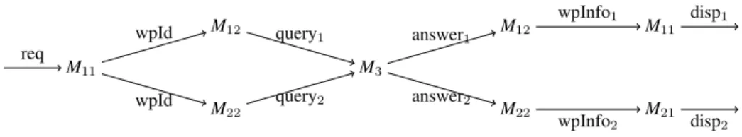
be displayed on the screen. This communication flows, from KC1 to MFD1 and MFD2

via the database, form two functional chains summarised in Figure 2.

Figure 2 The functional chains of the flight management system

M11 M12 M22 M3 M12 M22 M11 M21 req wpId wpId query1 query2 answer1 answer2 wpInfo1 wpInfo2 disp1 disp2 2.2.3 System requirements

These chains have to meet the following end-to-end temporal requirements:

• φL: pages relative to a pilot’s request must be displayed on each side within a

time window of 700 ms, meaning that the duration between treq, the date of the

pilot’s request, and tdispi, the time at which the requested information is

displayed, must satisfy

tdispi− treq ≤ 700 ms for i = 1, 2

• φC: the two pages on side 1 and 2 relative to a same pilot’s request must be

displayed in a bounded time window, more precisely:

| tdisp1− tdisp2 |≤ 300 ms.

φL is a worst case end-to-end latency requirement. φC is a worst case temporal

consistency requirement.

3 Worst case properties

In this section, we present our method to analyse temporal properties in networked real-time systems. We first model the behaviour of each element involved in the functional chain (modules, tasks, communication delays, . . . ) by a set of variables and constraints. The behaviour of the whole system is obtained by the conjunction of all these constraints. Using an objective function measuring the latency of the functional chain, we define a MILP which optimal solution gives the worst case latency of the chain. In the following, all variables used for offsets and dates are reals. All variables used to designate a specific hyper-period or a job interval are integers. We also use

Boolean variables for technical reasons. Although not mandatory, we only use integers for parameters in order to improve readability.

To capture the temporal behaviour of a functional chain,F =_{→ τ}a0

1

a1

→ ...τR aR →, we

need to ‘follow’ the propagation along the chain of an occurrence of an input a0 until

a related output aR is produced.

We then describe the case of latency in Section 3.2 and the specificities of consistency in Section 3.3.

3.1 Constraints and variables definition

We define the constraints and variables allowing to capture the expected behaviour of the modules, tasks and communications.

3.1.1 Module

Let Mi be a module. The only variable which characterises Mi is its possible offset

with respect to the other modules. Modules are asynchronous, thus the time origin of their execution frame may be shifted by an offset Oi. This offset may be arbitrary.

However, as we are interested in the regular behaviour, and not the specific case of the initialisation phase, it is not necessary to consider offsets greater than the maximal hyper-period of the system. The first constraints for Mi are then:

Oi∈ R, 0 ≤ Oi≤ max

k=0...mHk (1)

3.1.2 Task

In the following, we focus on a single task of the chain τj. The link with its previous

and next tasks in the chain is later realised with the constraints on the communication delays (see 3.1.3). Let τj ∈ F be a task of the functional chain executing on module

Mi, such as u

→ τj v

→, meaning the task consumes data u in order to produce data v. We

first describe how to capture the job and hyper-period of the task in which a specific occurrence of u is consumed. Then, we show how to constrain the production of the occurrence of v related to this u in order to follow the propagation of u through v.

3.1.2.1 Consumption of data

Let tu be the date where an occurrence of u is available on Mi. As presented in

Section 2.1, depending on the location of the task preceding τj, it may be delivered

by the network, or put in a shared memory of the module. To capture the temporal behaviour along the functional chain we need to link tu to the job of τj that

consumes this occurrence of u. From the task model, we have for each start of a job of τj:∃n ∈ N, ∃k ∈ 0..nj such that Oi+ nHi+ bkj(0), where Oi is the offset of the

module Mi, Hi its hyper-period, n the number of the current hyper-period and bkj(0)

u arriving at tu is consumed by the kth job of the task τj during the nth hyper-period of

Mi if and only if:

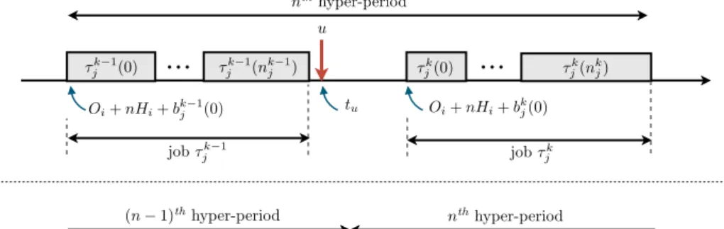
tu≤ Oi+ nHi+ bkj(0) { Oi+ nHi+ bkj−1(0) < tu ,∀k = 1..nj Oi+ (n− 1)Hi+ b nj j (0) < tu , for k = 0 (2)

as shown in Figure 3 there is a special case for k = 0, i.e., the first job of the hyper-period.

Figure 3 Special case for the first job of the hyper-period (see online version for colours)

u

...

...

...

...

In order to take into account these constraints into the MILP, we define a set of Boolean variables Ck

j, for all k = 0..nj (one Boolean per job, C stands for consumption). These

are indicator variables: Ck

j is true iff job τjk consumes the occurrence of u arrived at

time tu. The Boolean variables are constrained by:

nj

∑

k=0

C_jk = 1 (3)

meaning that one and only one job consumes u, and in order to respect the constraints (2), the Boolean variables are also constrained by:

tu≤ Oi+ nHi+ nj ∑ k=0 C_jk· bk_j(0) Oi+ nHi+ nj ∑ k=1 Ck· bkj−1− Infty · C 0 j < tu Oi+ (n− 1)Hi+ Infty· (Cj0− 1) + b nj j < tu (4)

where Infty is a large integer representing infinity. We use this large value in order to deal with the two cases of constraints (2). Indeed, if Cj0= 1 (meaning the consumer

job is τ0

j) then the second constraint is always true and the only active constraint is the

third one. Otherwise, if Cj0= 0 (meaning the consumer job is τjk, k = 1..nj) the third

constraint is always true and the second one is the only one active. As a result, for a given Oi and for a given tu (arrival of u), the previous constraints determine a single

n and a single k, i.e., the hyper-period and the job consuming u. 3.1.2.2 Production of data

We now capture the behaviour for the production of data v by task τj following the

consumption of an occurrence of u arrived at tu. Let tv be the date of this production

of v. Data can only be produced during one of the job intervals. If tv happens during

the nth _{hyper-period of M}

i and the lth interval of the kth job, then necessarily we have:

Oi+ nHi+ bkj(l)≤ tv≤ Oi+ nHi+ ekj(l) (5)

In order to take into account these constraints into the MILP, we use a set of Boolean variables Pjk(l), for all k = 0..nj and for all l = 0..nkj (one Boolean per job and per

interval, P stands for Production). These are indicator variables: Pjk(l) is true iff job

τ_jk produces the occurrence of v at time tv during interval [bkj′(l), e k

j′(l)]. Since the job

producing v is the same than the one which consumed u arrived at tu, the Boolean

variables are constrained by

C_jk−

nk_j

∑

l=0

P_jk(l) = 0,∀k = 0..nj (6)

We show that the constraints (6) model the link between the job consuming u arrived at tu and the interval of the job producing v. Let k = 0..nj be a job, if Cjk= 0 then

necessarily, ∀l = 0..nkj, P k

j(l) = 0, meaning that no interval of job k produces the

occurrence of v we want to follow. Conversely, if Cjk = 1 then necessarily,∃l = 0..n k j,

P_jk(l) = 1, and ∀l′= 0..n_jk, l′̸= l, P_jk(l′) = 0 meaning that one and only one interval of job k produces v. From constraint (4), we know that only one job k can consume u. Thus, the constraints model the expected behaviour.

We now use the Boolean variables Pjk(l) to constrain tu to happen during the

interval selected by the previous constraints:

Oi+ nHi+ nj ∑ k=0 nk j ∑ l=0 P_jk(l)· bk_j(l)≤ tv tv ≤ Oi+ nHi+ nj ∑ k=0 nk_j ∑ l=0 Pjk(l)· e k j(l) (7)

3.1.3 Communication delay

The communication constraints link the tasks in the chain. We describe this link between a task τj producing v and τj′ consuming v: τj

v

→ τj′. Two cases arise for the

communication delay. Either the communication between τj and τj′ happens through

the network or, if the tasks execute on a common module, through a shared memory. Let

toutv be the time at which τj produces data v (it was noted tv in the previous constraints)

and tin

v be the time at which v is available for consumption in the module of τj′.

3.1.3.1 Communication through a timed channel

As presented previously, communications through the network are abstracted with a timed channel characterised by a communication delay in [δmin, δmax]. Hence, toutv and

tin

v are constrained by:

tout_v + δ_min≤ tin_v

tinv ≤ toutv + δmax

(8)

3.1.3.2 Communication through shared memory

If the communication is realised through a shared memory, then it is considered instantaneous. Hence, we have:

tout_v = tin_v (9)

a shared memory is similar to a timed channel characterised by the interval [0, 0].

3.2 Objective function: worst case latency

LetF =a0

→ τ1

a1

→ ...τR aR

→ be a functional chain. The possible behaviour of this chain is

obtained by the conjunction of all the constraints of all the tasks and the communication involved in the chain. The set of constraints thus obtained forms a MILP (because some variables are reals and some are integers). Let us note t0 the arrival date of a0, and tR

the production date of aR. Then the latency of the chain is

L = tR− t0

The worst case latency is obtained on a particular behaviour maximising L. This behaviour can be found by using a MILP solver with the objective function:

maximise: tR− t0

3.3 Objective function: worst case consistency

In this section, we detail the specificities of the proposed MILP formulation for the worst case consistency analysis. We consider a set of functional chains F1, . . . ,FK.

For all c = 1..K, we note Rc the number of task inFc. Every functional chain has the following form: Fc= ac,0 → τc,1 ac,1 → . . .ac,Rc−1 → τc,Rc ac,Rc → (10)

We are interested in the temporal consistency of divergent chains, thus all chains share a common first element: ∀(c, c′)∈ [1..K]2, ac,0= ac′,0.

Temporal consistency measures the distance between the outputs of functional chains relating to a common input. Let t1,R1, . . . , tK,RK be the dates of such outputs. All these

dates depend on a common initial date t0which corresponds to an arrival at the input of

the chains. t0is also a variable of the problem. Moreover, the dates are constrained with

the same constraints as for the latency. The worst case consistency is then the maximum distance between the largest tc,Rc,∀c = 1..K and the smallest one. More precisely, the

objective is:

maximise: max

c=1..K{tc,Rc} − minc=1..K{tc,Rc} (11)

However, this objective is not linear and cannot be used in a MILP. In the following, we propose a linearisation of this objective function. First, we define two technical variables (maxT, minT)∈ R2_{. They represent respectively the maximum and minimum dates of}

the outputs. The objective becomes:

maximise: maxT− minT (12)

Then, we add some constraints to ensure that at least one of the dates is equal to maxT and one of the dates is equal to minT. Since the objective is a maximisation, the solver will choose the largest value for maxT and the smallest for minT. We start with maxT. For each tc,Rc, c = 1..K, we add the two following constraints:

maxT≤ tc,Rc+ (1− B maxT c )· Infty maxT≥ tc,Rc− (1 − B maxT c )· Infty (13) where BmaxT

c is a Boolean variable and Infty is a large integer representing infinity. If

BmaxT

c = 1 then necessarily tc,Rc= maxT. Otherwise the variable tc,Rc is free. We also

add the following constraint to ensure that at least one variable BmaxT

c is equal to 1: K

∑

c=1

B_cmaxT≥ 1 (14)

We proceed in a similar manner to constrain the value of minT. For each tc,Rc, c = 1..K,

we add the following constraints:

minT≤ tc,Rc+ (1− B minT c )· Infty minT≥ tc,Rc− (1 − B minT c )· Infty K ∑ c=1 B_cminT≥ 1 (15)

The linearisation of the objective function results in the addition of two real variables, 2K Boolean variables and 4K + 2 constraints.

4 Discussions

The purpose of this section is to discuss several aspects of our approach. First, we benchmark our global approach against a local approach for the latency and consistency properties. The gain we achieve is intuitively explained in a simple example. The improved tightness of the analysis comes at a price: complexity. Our global approach involves solving a MILP. It is obviously more complex than a local approach that typically involves analytical formulas. We run several experiments to test the scalability of our approach. Finally, we consider that a key feature of our work is its flexibility. We show how it can be extended to analyse other properties. As an example, we propose an extension to best case latency and best case consistency evaluations.

4.1 Local vs. global analysis

For each property, we first give results for a local approach. These results are similar to formulas used in Al Sheikh et al. (2012) for latency and in Pontisso et al. (2010) for consistency. However, we specialise these local approaches to our model.

4.1.1 Worst case latency

As described in the related works, a local approach consists in determining worst case response time (WCRT) of each component visited by the functional chain, then the end-to-end latency is the sum of the WCRT.

4.1.1.1 Local Worst Case Latency

The WCRT of a timed channel ci is the upper bound of the communication delay:

δmax

i . If we note WCRT(τj) the worst case response time of a task τj, then with a local

approach an upper bound of worst case latency of a functional chainF =_{→ τ}a0

1

a1

→ ...τR aR

→ which uses a set c1, . . . , clof timed channels to communicate is:

WCL(F) = R ∑ j=1 WCRT(τj) + l ∑ j=1 δ_jmax (16)

In our model, the WCRT of a job τk

j of a task τj happens when a data waits the longest

possible time before being acquired by the job and the processing in the job takes the longest possible time. This scenario occurs when the data arrives just after the beginning of the first interval of the previous job, and the production happens at the end of the last interval, as shown in Figure 4 (u represents the data and v the resulting data of its processing by τjk). Taking into account the hyper-period of the module Mi hosting the

task, the WCRT of this job is then:

( ekj(nkj)− b p(k) j (0) ) mod Hi, p(k) = { k− 1 if k > 0 nj if k = 0 (17)

Figure 4 Local worst case scenario for the job τk

j (see online version for colours) ⇣ ek j(nkj) bp(k)j (0) ⌘ mod Hi bk j(nkj) ekj(nkj) bp(k)_j (0) ⌧k j(nkj) ⌧k j(0) ⌧jp(k)(n p(k) j ) u v

...

...

The worst case response time of a task τj is the maximum response time of all its jobs:

WCRT(τj) = max k=0..nj {( ek_j(nk_j)− bp(k)_j (0) ) mod Hi } (18)

For example, in the case study the task WaypointM is characterised by two jobs

{[15, 31]} and {[60, 76]} (only one interval per job) on the hyper-period H2= 120.

Thus, WCRT(WaypointM) = max{(31 − 60) mod 120, (76 − 15) mod 120} = max{91, 61} = 91

To be fair with the local approach, we use the following idea: because of the scheduling of the navigation database tasks, the result of the first (resp. second) job of

NDBReqM is necessarily processed in the first (resp. second) job of NDBServ and which

result is then processed in the first (resp. second) job of NDBRep. Thus, this sequence of tasks can be considered as only one task with two jobs per hyper-period. The beginning of the first (resp. second) job is the beginning of the first job (resp. second) of

NDBReqM and the end of the first job (resp. second) job is the end of the first job (resp.

second) of NDBRep. In the following, we name this task NDB and it is characterised by the intervals: [0, 54], [102, 156]. Table 1 provides the WCRT considered for the tasks.

Table 1 Worst case response time of the case study tasks

Task KC CockpitReqM NDB WayPointM MFD

WCRT 55 85 156 91 62

4.1.1.2 Local vs. global worst case latency

We compare the global approach against the local one by varying the upper bound of the communication delays (for simplicity we assume that all the δmax

i are equals).

The results are plotted in Figure 5. According to equation (16) the worst case latency determined with the local approach is linear (straight dashed line). The results of the global approach form a step function which is right continuous: for example

∀δmax

i ∈ [0, 15), W CL = 403, ∀δ max

i ∈ [15, 22), W CL = 443...

We can see on the results that the global approach provides more accurate results than the local approach. The curve of the global approach varies by steps. One of the reason is that the involved functional chain crosses twice the modules M1 and M2.

Consider a part of the worst case scenario depicted in Figure 6. The task CockpitReqM (noted CRM) on module M2 sends a query to the task NDB on module M3, the answer

is then processed by the task WaypointM (noted WP) on module M2 resulting in an

not change which job of WP processes NDB answers. Thus, the end-to-end latency is unaffected by variations of the worst case communication delay. In the case of the local approach, it is the job with the worst case response time which is always assumed to process the data. Which also explains the improvement obtained by the global approach.

Figure 5 Results of the case study – global vs. local approach (see online version for colours) 0 20 40 60 400 500 600 700

Communication delay δmax

i (ms) WCL ( F1 ) (ms)

Worst case latency (ms)

400 500 600 700 WCL ( F1 ) (ms)

Figure 6 Interpretation of the global approach curve

CRM WP … CRM WP query δmax NDB NDB … … answer δmax wpInfo

System designers could take advantage of this more accurate evaluation technique: within certain range they could increase the network load with no impact on high-level requirement, which could be crucial for future evolution of the system.

To confirm the trend in this results, we extend the case study to build two experiments:

• A module M3′, similar to M3, is added. The tasks of M3′ correspond to the

navigation database tasks and as for M3 we consider them as a bundle of tasks

noted NDB’. The functional chain considered is then:→ KCreq wpId→ CockpitReqM

query

→ NDB answer

→ NDB’answer’

→ WayPointMwpInfo→ MFDdisplay→ .

• A module M2′, similar to M2, is added. The tasks of M2′ correspond to the flight

management tasks of M2. In particular, we add the tasks CockpitReqM’ and

WayPointM’ to the functional chain. The goal is to add a module which is crossed

twice. The functional chain considered is then:→ KCreq wpId→ CockpitReqM query→

The results of these experiments are plotted in Figures 7 and 8 respectively.

The improvement of the global approach is more important with the experiment 2. Indeed, the module added to the case study is crossed twice by the functional chain and so the benefit of the approach (as presented in Figure 6) is more significant. These results indicate that the more modules are crossed multiple time by the functional chain, the more the proposed approach may be relevant.

Figure 7 Results with module M3′ added (see online version for colours)

0 20 40 60 500 600 700 800 900

Communication delay δmax

i (ms) WCL ( F 1 ) (ms)

Worst case latency (ms)

500 600 700 800 900 WCL ( F 1 ) (ms)

Figure 8 Results with module M2′ added (see online version for colours)

0 20 40 60

600 800

Communication delay δmax

i (ms) WCL ( F 1 ) (ms)

Worst case latency (ms)

600 800 WCL ( F 1 ) (ms)

4.1.2 Worst case temporal consistency

An upper bound on the worst case consistency is given by the maximum difference between the worst case and best case latency of the functional chains. Thus, to express this bound we first need to define a lower bound on the best case latency of a chain.

4.1.2.1 Local best case latency

For the local approach, the best case response time (BCRT ) of a job of a task happens when data arrives just before the beginning of the job and the data is processed with minimum delay. In our model, no minimum delay is defined, thus processing can be instantaneous. The best case latency is then reduced to the sum of the lower bound of the communication delays. For a functional chain F =_{→ τ}a0

1

a1

→ ...τn an

→ which uses a

set c1, . . . , cl of timed channels to communicate, we have:

BCL(F) =

l

∑

j=1

δ_jmin (19)

Note that a minimal processing delay could be included in our model without technical difficulty.

4.1.2.2 Local worst case consistency

With a local approach, we can obtain the following upper bound for the consistency of the functional chains F1, . . . ,FK:

WCC(F1, . . . ,FK) = max c=1..K { WCL(Fc) } − min c=1..K{BCL(Fc)} (20)

4.1.2.3 Local vs. global worst case consistency

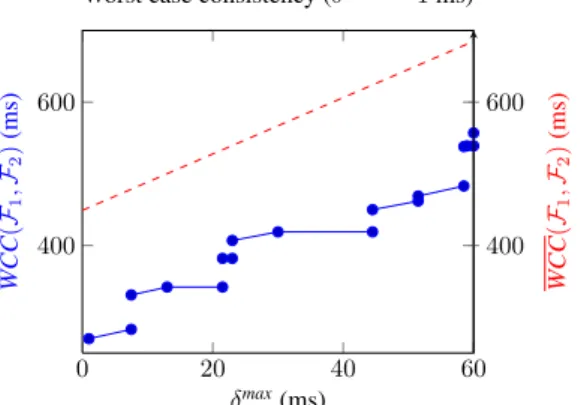
As for the worst case latency, we compare the global approach against the local one by varying the upper bound δmax of the communication delays. The lower bound of the

communication delays is assumed to be constant δmin= 1ms. The results are plotted in

Figure 9.

Figure 9 Worst case consistency – global vs. local approach (see online version for colours)

0 20 40 60 400 600 δmax_(ms) WCC ( F 1 , F2 ) (ms)

Worst case consistency (δmin

= 1 ms) 400 600 WCC ( F 1 , F2 ) (ms)

4.2 Scalability

We have developed a prototype which takes the description of a system and a set of functional chains as inputs. It automatically generates the MILPs to determine the worst case latency of a chain or the worst case consistency of a set of chains. Then, the MILPs are solved with the open source solver lp solve. Experiments run on a Intel Core 2 Duo 2.53 GHz processor.

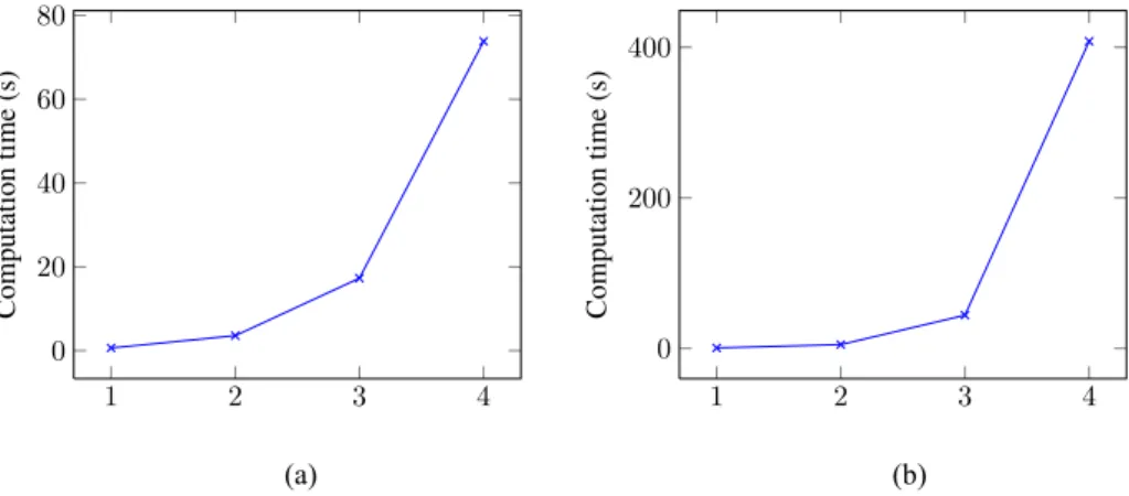
To find the limiting factors of the approach, we further extend the case study. In Figure 10(a) we add up to four modules with navigation database tasks and we plot the required computation time to the corresponding MILPs. In Figure 10(b) we add up to four modules with flight management tasks and we plot the required computation time to solve the corresponding MILPs. For the consistency, we both increase the length of the functional chains by adding NDB modules and increase the number of functional chains by duplicating the modules. The corresponding computation times are plotted in Figure 11.

Figure 10 Worst case latency computation time, (a) number of NDB modules (b) number of FM modules (see online version for colours)

1 2 3 4 0 20 40 60 80

(a) Number of NDB modules

Computation time (s) 1 2 3 4 0 200 400 (b) Number of FM modules Computation time (s) (a) (b)

Figure 11 Worst case consistency computation time – for K functional chains (see online version for colours)

1 2 3 0 100 200 300 Number of NDB modules Computation time (s) K = 2 K = 3

In all these cases, the required computation time increases exponentially with the number of added modules. This is due to the fact that for each added task, n binary decision variables must be added to the MILP (with n the number of interval characterising the task). Remember that these binary variables are used to decide which job in the hyper-period of the task module is involved in the functional chain. Solving the MILP for the consistency is also more complex for two reasons:

1 Boolean variables have been added to linearise the objective function (c.f., Section 3.3).

2 The problem is highly symmetrical. This is known to be a burden for solvers.

We can also notice that solving the MILP for the experiments with a module similar to M2 (flight management module) is more difficult. Let us consider again the scenario

depicted in Figure 6. Finding the jobs of CRM and WP involved in the worst case depends on the time elapsed between the production of the query and the reception of the answer. Thus, inter-dependencies exist between part of the functional chain and the MILP becomes more complex to solve.

4.3 Extension to best case evaluation

One advantage of the proposed approach is that it is easily extendable. Indeed, it allows to evaluate other relevant properties like the minimum latency or consistency of the functional chains for instance. A classical example of system which must verify a minimum and a maximum latency is an airbag: upon a collision, it must neither be inflated too early nor too late. We first present the ideas for extending our approach to best case latency and compare the results to a local approach. Then we discuss the specificities of the best case consistency.

4.3.1 Best case latency

To apply our approach to the best case latency, we can reuse the MILP defined for the worst case. We just need to change the objective function to:

minimise: tR− t0 (21)

As for the worst case latency, we compare a local approach with a global approach. We use the same methodology as with the worst case to benchmark the global approach against the local one. Increasing the upper bound of communication delay does not impact the best case latency, thus only the lower bound (δmin

i ) is varying. The results

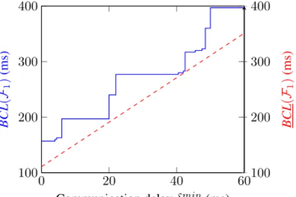
are plotted in Figure 12. The straight dashed line corresponds to the local approach. Because some steps of the results of the global approach are small, we do not plot the discontinuities (i.e., the jumps of the function). The function is left continuous. We can see the global approach improves the analysis of best case latency. The reasons are similar to the analysis of the worst case.

Figure 12 Best case latency – global vs. local approach (see online version for colours) 0 20 40 60 100 200 300 400

Communication delay δmin

i (ms) BCL ( F1 ) (ms) 100 200 300 400 BCL ( F1 ) (ms)

4.3.2 Best case consistency

The best case consistency is the minimum distance between the outputs of the functional chains:

minimise: max

c=1..K{tc,Rc} − minc=1..K{tc,Rc} (22)

The concept of best case consistency is less intuitive than the worst case, we give an illustration in Figure 13. The consistency of 3 functional chains F1,F2 and F3 are

considered. The ranges of possible values for the outputs t1,R1, t2,R2 and t3,R3 are represented. These ranges depend on the constraints of the MILP. On this example, the best case consistency is obtained by giving the largest possible value to t3,R3, the smallest one to t2,R2 and any value in between to t1,R1.

Figure 13 An example of best case consistency

F1 F2 F3 BCC_(F1, F2, F3) t1,R₁ t2,R₂ t3,R₃ : : :

As for the maximisation problem, two technical variables maxT and minT are introduced to linearise the objective function:

minimise: maxT− minT (23)

and the same constraints (13), (14) and (15) are used. However, to apply our approach to the best case consistency, some constraints must be added to the MILP used for

the worst case. Indeed, otherwise for the minimisation solver could assign the minimal value to maxT and the maximal one to minT. For each tc,Rc, c = 1..K, we add the two

following constraints:

maxT≥ tc,Rc minT≤ tc,Rc

(24)

thus, maxT is constrained to be equal to the largest tc,Rc and minT is constrained to

be equal to the smallest tc,Rc. Applied to the case study, the best consistency is always

null. This is because the problem is highly symmetrical and the data can be produced at the output at exactly the same time.

5 Conclusions and perspectives

The article presents an analysis method for end-to-end freshness and end-to-end temporal consistency properties on GALTT systems. This verification method is based on a MILP modelling. Worst case end-to-end properties are computed as optimal solutions of the MILP problem. An interesting feature of this approach is that it computes more accurate temporal bounds than local approaches as shown in Section 4.1. Another interesting point, as shown in Section 4.3, is its flexibility: one can easily compute best case end-to-end bounds by only modifying the objective function of the MILP form max to min. From a scalability point of view, the case study considered previously is composed of 11 tasks. This case study is representative from industrial systems (usually composed of 5 to 10 tasks). Our method applied to this case study does not take more than 1s for the latency or consistency analysis (with a non-optimised solver). We think that these results are promising.

In this article, we made however a strong hypothesis about the internal behaviour of the tasks. We implicitly considered that each job of each task does not induce a delay greater than its worst case response time, i.e., the end of its last time interval. Obviously it is not always the case in realistic systems. Some tasks can implement ‘confirmation tests’ waiting for a given amount of time (generally a multiple of its period) before producing a consolidated output. Obviously this internal latency impacts the global latency and the global consistency of the chain. Our next work is to extend our global method by tasks involving internal delays.

References

Al Sheikh, A., Brun, O., Hladik, P-E. and Prabhu, B.J. (2012) ‘Strictly periodic scheduling in IMA-based architectures’, Real-Time Systems, Vol. 48, No. 4, pp.359–386.

ARINC 653 (1997) ARINC 653 – Avionics Application Software Standard Interface,

Aeronautical Radio Inc.

Bauer, H., Scharbarg, J-L. and Fraboul, C. (2009) ‘Applying and optimizing trajectory approach for performance evaluation of AFDX avionics network’, in Proceedings of the 14th IEEE

International Conference on Emerging Technologies & Factory Automation, ETFA ‘09,

pp.690–697, IEEE Press, Piscataway, NJ, USA.

Boniol, F., Pagetti, C., Lauer, M. and Ermont, J. (2012) ‘End-to-end latency analysis in networked real-time systems’, in VECoS 2012 – 6th International Workshop on Verification

and Evaluation of Computer and Communication Systems, Electronic Workshops in Computing (eWiC), BCS, September.

Carcenac, F. and Boniol, F. (2006) ‘A formal framework for verifying distributed embedded systems based on abstraction methods’, International Journal on Software Tools for

Technology Transfer, November, Vol. 8, No. 6, pp.471–484.

Chokshi, D.B. and Bhaduri, P. (2010) ‘Performance analysis of flexray-based systems using real-time calculus, revisited. ‘In Sung Y. Shin, Sascha Ossowski, Michael Schumacher, Mathew J. Palakal and Chih-Cheng Hung (Eds.): SAC, pp.351–356, ACM.

Cucu-Grosjean, L. and Buffet, O. (2009) ‘Global multiprocessor real-time scheduling as a constraint satisfaction problem’, in Leonard Barolli and Wu Chun Feng (Eds.): ICPP

Workshops, pp.42–49, IEEE Computer Society.

Ferrandiz, T., Frances, F. and Fraboul, C. (2011) ‘Worst-case end-to-end delays evaluation for spacewire networks’, Discrete Event Dynamic Systems, Vol. 21, No. 3, pp.339–357. Herpel, T., Hielscher, K-S.J., Klehmet, U. and German, R. (2009) ‘Stochastic and deterministic

performance evaluation of automotive can communication’, Computer Networks, Vol. 53, No. 8, pp.1171–1185.

Jha, A.K., Xiong, M. and Ramamritham, K. (2006) ‘Mutual consistency in real-time databases’, in Proceedings of the 27th IEEE International Real-Time Systems Symposium (RTSS ‘06), Rio de Janeiro, pp.335–343, December, IEEE Computer Society, Washington, DC, USA. Le Boudec, J-Y. and Thiran, P. (2001) ‘Network calculus’, Lecture Notes in Computer Science

(LNCS), Springer Verlag.

Martin, S. and Minet, P. (2006) ‘Worst case end-to-end response times of flows scheduled with FP/FIFO’, in Proceedings of the International Conference on Networking, International

Conference on Systems and International Conference on Mobile Communications and Learning Technologies, pp.54–62, April, IEEE Computer Society, Washington, DC, USA.

Navet, N. and Simonot-Lion, F. (2008) ‘A review of embedded automotive protocols’, in Nicolas Navet and Franc¸oise Simonot-Lion (Eds.): The Automotive Embedded Systems

Handbook, Industrial Information Technology Series, Taylor & Francis/CRC Press.

Pontisso, N., Qu´einnec, P. and Padiou, G. (2010) ‘Analysis of distributed multi-periodic systems to achieve consistent data matching’, in Khalil Drira, Ahmed Hadj Kacem and Mohamed Jmaiel (Eds.): NOTERE, pp.81–88, IEEE.

Sagaspe, L. and Bieber, P. (2007) ‘Constraint-based design and allocation of shared avionics resources’, in 26th AIAA-IEEE Digital Avionics Systems Conference, Dallas.

Sha, L., Abdelzaher, T., AArz´en, K-E., Cervin, A., Baker, T., Burns, A., Buttazzo, G., Caccamo, M., Lehoczky, J. and Mok, A.K. (2004) ‘Real time scheduling theory: a historical perspective’, Real-Time Syst., November, Vol. 28, Nos. 2–3, pp.101–155.

Sofack, W.M. and Boyer, M. (2012) ‘Non preemptive static priority with network calculus: enhancement’, in Jens B. Schmitt (Ed.): MMB/DFT, pp.258–272, Vol. 7201 of Lecture Notes

in Computer Science, Springer.

Song, X. and Liu, J.W.S. (1995) ‘Maintaining temporal consistency: pessimistic vs. optimistic concurrency control’, IEEE Transactions on Knowledge and Data Engineering, October, Vol. 7, No. 5, pp.786–796.

Spuri, M. (1996) Holistic Analysis for Deadline Scheduled Real-Time Distributed Systems, Research Report RR-2873, INRIA, Project REFLECS.

Thiele, L., Chakraborty, S. and Naedele, M. (2000) ‘Real-time calculus for scheduling hard real-time systems’, in ISCAS, pp.101–104.

Tindell, K. and Clark, J. (1994) ‘Holistic schedulability analysis for distributed hard real-time systems’, Microprocessing and Microprogramming, Vol. 40, Nos. 2–3, pp.117–134.