OATAO is an open access repository that collects the work of Toulouse
researchers and makes it freely available over the web where possible
Any correspondence concerning this service should be sent
to the repository administrator:
[email protected]
This is a publisher’s version published in:
http://oatao.univ-toulouse.fr/24151
To cite this version:
Picot, Antoine and Malec, David and Maussion, Pascal
Improvements on lifespan modeling of the insulation of low
voltage machines with response surface and analysis of
variance. (2013) In: SDEMPED 2013, 27 August 2013 - 30
August 2013 (Valencia, Spain).
Official URL:
https://doi.org/10.1109/DEMPED.2013.6645777
Improvements on Lifespan Modeling of the
Insulation of Low Voltage Machines with
Response Surface and Analysis of Variance
Antoine Picot, David Malec and Pascal Maussion
1Abstract- The aim of this paper is to present some improvements of the method for modeling the lifespan of insulation materials in a partial discharge regime. The first step is based on the design of experiments which is well-known for reducing the number experiments and increasing the accuracy of the model. Accelerated aging tests are carried out to determine the lifespan of polyesteimide insulation films under different various stress conditions. A lifespan model is achieved, including an original relationship between the logarithm of the insulation lifespan and that of electrically applied stress and an exponential form of the temperature. The significance of the resulting factor effects are tested through the analysis of variance. Moreover, response surface is helpful to take into account some second order terms in the model and to improve its accuracy. Finally, the model validity is tested with additional points which have not been used for modeling.
Index terms—Diagnosis, dielectrics, insulation, insulation testing,
accelerated aging, lifespan estimation, condition monitoring, modeling, aging, response surface, analysis of variance (ANOVA)
I. NOMENCLATURE
Ei Effect of factor number i
Eii Effect of the square of factor number i
Eij Effect of interaction between factor number i and
factor number j n Number of experiments
Fi Level of factor i, could be +1, -1 or any value between
-1 and +1
Ê Effect vector composed of the different Eij terms
X Experimental matrix
Y Y is the experimental Weibull’s vector M Average experimental value
L Lifespan in minutes T Temperature in °C V Voltage in V F Frequency in Hz VA N k n0 dof Variance of factor A
Number of samples = number of repetitions Number of factors (k=3)
Number of center points Degrees of freedom
1
Authors are with Université de Toulouse ; INPT, UPS ; LAPLACE (LAboratoire PLAsma et Conversion d’Energie); ENSEEIHT, 2 rue Charles Camichel, BP 7122, F-31071 Toulouse cedex 7, France and CNRS; LAPLACE; F-31071 Toulouse, France.
II. INTRODUCTION
Low voltage electric machines are increasingly submitted to heavy electric constraints and their lifespan becomes nowadays a concern. Among many papers, [1] have reported that stator-winding insulation is one of the weakest components in a drive (around 40% of failures). Materials involved in electric ageing affect the insulation system lifespan. Many operating factors such as voltage, frequency, temperature, pressure, etc. could have a dramatic effect as these stresses can synergize as shown in [2]. The existing models of degradation or of lifespan differ slightly from one paper to another but they are all based on physics and include some factors which are specific to the material or the aging mechanism. As examples, [3]-[4] include the physical, thermal and electro-mechanical aspects of the electrical aging process. Additionally, the choice of the lifespan forms remains critical for model accuracy. Various forms can be found in different works such as [5] where they mainly involve a log-based relationship for frequency and voltage and an exponential form for the temperature. Nevertheless, there is no comprehensive model for insulation lifespan prediction under different combined stresses and this phenomenon remains complex and difficult to understand and to model, especially with PWM supply.
Experimental tests are necessary to assess lifespan modeling but full aging tests for all the factors involved in the aging process under nominal conditions could be time consuming. As a consequence, accelerated aging tests which are about to speed up the degradation, are generally performed in order to study and predict the lifespan.IGBT modules in high temperature power cycling are tested in [6] whereas nano-structured enamels on twisted pairs are tested in [7] under severe waveforms but it does not give any lifespan model.
The “Design of Experiments” (DoE) [8] was helpful in many cases either for optimization or modeling purposes. The principle of this methodology is to organize and carry out just the required number of experiments in order to obtain the most accurate information for a specific problem. Its performance has been put in evidence in different applications, especially in chemistry and mechanics, where a high volume of parameters have to be simultaneously optimized. In recent years, DoE have been successfully used
in electrical engineering for electrical machine design (induction, reluctance, synchronous…) [9]-[11] or for the control of power electronic devices [12]-[13]. In the field of insulation lifespan modeling, [14] provides a model with some statistical analysis to test which parameters are significant or not. A set of 8 tests are carried out for each combination of the stress factors (Voltage, Temperature and Frequency). To be more cost effective, this paper will try to reduce this number of tests. But, it is important to check whether the results remain statistically significant or not and Analysis of Variance (ANOVA) will be employed.
III. SYSTEM DESCRIPTION AND BASIC DOE The testbench itself and the tested insulation materials have been fully described in [14]. It consist of steel plates coated with polyesterimide (PEI - thermal class: 180°C) films which are widely used in rotating machine insulation systems (15cm x 9cm with a 90µm coating).
Fig. 1. Tested 90µm coated steel plate (15cm x 9cm)
Eight samples were tested in our experimental setup, shown in Fig.2. Under electrical stress, the steel plate acts as the first electrode and a spherical stainless steel electrode (diameter: 1mm) is the second. Samples were placed in a climatic chamber where the temperature is fully controlled. The lifespan of each sample was measured using a timer (one per sample) which stopped counting as soon as the current increased and crossed a threshold at which the corresponding sample broke down. The faulty specimen was disconnected while the survivors remained under voltage and at the controlled temperature. Accelerated aging tests are carried out in order to relate the applied external stresses (factors) to the insulation lifespan (response). Lifespan data in this paper is presented according to Weibull’s statistical processing [15], which is commonly used for breakdown data treatment.
Fig. 2. The experimental setup for accelerated aging tests, climatic chambers and power electronic.
The failure process is driven by several stresses acting simultaneously such as electrical, thermal, mechanical and ambient stresses. The experimental aging conditions of theses accelerated tests were chosen to ensure that the insulation degradation is mainly due to the partial discharges. However, for simplicity and because of their influence, only three major parameters were studied:
1) the square wave applied HVDC (V), 2) the frequency of the applied voltage (F), 3) temperature (T).
TABLEI
LEVELS OF THE THREE STRESS FACTORS
Factors Level (-1) Level (+1) Level (0)
Log (Voltage (kV)) Log(1) Log(3) Log(1.73)
Log((Frequency (kHz)) Log(5) Log(15) Log(8.7)
Exp(-b.Temperature
(°C)) Exp(55b) Exp(-180b) Exp(26.7b)
with b= 5.64x10⁻³
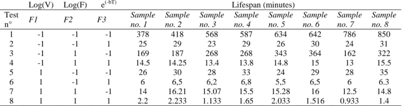
The basic data treatment of the PEI insulation film lifespan relies on the Design of Experiments as written in [16] and [14]. The corresponding plans and results are recalled in Table II and Table III for an easy understanding. Table II gives all the 23 (3 factors, 2 levels each) possible combinations between the different factor levels whereas Table III list the sample lifespans (in minutes). They lead to a first model presenting a logarithmic form of electrical stress (i.e. voltage and frequency) and an exponential form of the temperature as expressed in (1). The coefficients of the model are listed in Table IV.
Log(L) ~ M + EV.log(V) + EF.log(F) + ET.exp(-bT) +
EFV.log(V).log(F) + EVT.log(V).exp(-bT) +
EFT.log(F).exp(-bT) + EVFT.log(V).log(F).exp(-bT)
TABLE II
EXPERIMENTAL RESULTS WITH THREE FACTORS AT 2 LEVELS EACH :8 EXPERIMENTS WITH 8 SAMPLES EACH
Log(V) Log(F) e(-bT) Lifespan (minutes)
Test n° F1 F2 F3 Sample no. 1 Sample no. 2 Sample no. 3 Sample no. 4 Sample no. 5 Sample no. 6 Sample no. 7 Sample no. 8 1 -1 -1 -1 378 418 568 587 634 642 786 850 2 -1 -1 1 25 29 23 29 26 30 24 31 3 -1 1 -1 169 187 268 268 343 364 162 322 4 -1 1 1 14.5 14.25 13.4 13.8 14.8 15 13 15.5 5 1 -1 -1 26 30 28 33 24 29 28 35 6 1 -1 1 6 6,5 6,2 6,8 5,5 6,5 6 6.3 7 1 1 -1 14 16.21 15.07 15.5 15.28 16 12.5 14.8 8 1 1 1 2.2 2.233 1.133 1.65 2.033 1.516 0.933 1.4 TABLE III
FULL FACTORIAL DESIGN MATRIX FOR THREE FACTORS WITH 2 LEVELS EACH
Log(V) Log(F) e(-bT) Log(V).Log(F) Log(V).e
(-bT) Log(F). e(-bT) Log(V).Log(F) .e(-bT) Log(L) Test
n° M F1 F2 F3 I(V.F) I(V.T) I(F.T) I(V.F.T) Weibull
1 1 -1 -1 -1 1 1 1 -1 2.824 2 1 -1 -1 1 1 -1 -1 1 1.453 3 1 -1 1 -1 -1 1 -1 1 2.459 4 1 -1 1 1 -1 -1 1 -1 1.167 5 1 1 -1 -1 -1 -1 1 1 1.486 6 1 1 -1 1 -1 1 -1 -1 0.806 7 1 1 1 -1 1 -1 -1 -1 1.187 8 1 1 1 1 1 1 1 1 0.255
Tests at the center of the study domain
Model : Log(L)=f[Log(V), Log(F) and exp(-b.T)]
9 1 0 0 0 0 0 0 0 1.43
The factor effect calculation can be achieved by a simple matrix inversion through the following relationship (2), where (Ê) is the 8x1 effect vector, Y is the 8x1 experimental Weibull’s vector of the and X is the 8x8 matrix composed of experiment levels, the dark grey part in Table III.
Ê = X-1.Y (2)
TABLEIV
EFFECT VALUES FOR THE LIFESPAN MODEL, VECTOR Ê
Model Effect M 1.45 Log(V) -0.53 Log(F) -0.19 Exp(-bT) -0.54 ILog(V).Log(F) -0.03 ILog(V).exp(-bT) 0.12 ILog(F). exp(-bT) -0.03 ILog(F).Log(F). exp(-bT) -0.05
Once this factors have been calculated as in any kind of regression problem, tests of hypotheses are helpful in measuring their usefulness and whether their contribution to the model are significant or no. The following section describes the analysis of variance which is carried out as test of significance.
IV. SIGNIFICANCE AND REPETITION NUMBER USING
ANOVA
A. ANOVA presentation
ANOVA is a widely used statistical model separating the total variability found within a data set into two components: random and systematic factors. It has been demonstrated in [17] that ANalysis Of Variance (ANOVA) is a very interesting technique to assess the statistical significance of the different factor effects in many different applications in the wide field of electrical engineering. A new rotor shape for a high-speed interior permanent-magnet synchronous motor is presented in [18]. Its design is based on a full factorial experimental design and leads to a significant reduction in the amount of permanent magnet
employed. Moreover, the design factors of the greatest influence are identified with the help of ANOVA. This method has also been used in [19] in order to evaluate student’s performance in tests and exams after supervisory control and data acquisition (SCADA) and robotics experiments in control and automation education. The study put in evidence the usefulness of experimental practice even on low cost experimental setups. Energy production from PV generators is monitored in [20] and ANOVA helps to get concise information about the energy produced by all the inverters for comparison purposes.
B. Significance and ANOVA
Some of the factor effects computed in the ageing model proposed in section I are close to 0. These effects might not be significant and might be only due to the variability of the data, i.e. caused by non-controlled factors. To use ANOVA, two conditions must be verified:
• data must be normally distributed for each factor, • the different data must be independent.
Variance Vi due to the specific factor i is compared to
the variance of the data set, called the residual variance Vr.
If the factor is not significant, the variance Vi will be very
close to Vr. On the contrary, the variance V1 will be
proportionately higher than Vr. The ratio Fexp=Vi/Vr is
computed and tested using a Fisher-Snedecor test. This method tests the equality of both variances. So, the null hypothesis is to consider the effect of A as non-significant. In this case, the ratio Fexp should be less than a threshold
Flim. The effect of A is considered as statistically significant
if Fexp is greater than Flim. The threshold Flim is defined
according to the table of upper critical values of the F-distribution depending on the degrees of freedom of the data and the test significance level (generally fixed at 5%). For each test, a residue rij is computed as the difference between
the lifetime obtained for a particular repetition j and the average lifetime obtained for this particular experiment i. The residual variance Vr is computed for all experiments i
and repetitions j according to (3):
V ∑ (3)
where dofr is the number of degrees of freedom for the
residues. If we consider a DoE with N experiments and k repetitions for each test, the degrees of freedom for each test will be equal to k-1 and so the number of degrees of freedom for the residues will be dofr=N(k-1). For each
factor i, a variance Vi is computed as follows:
∑ (4)
where n is the number of tests when factor Fi is to a certain
level, Ei is the effect of the factor i and dofi its number of
degrees of freedom. The number of tests n can be computed as the total number of tests N.k divided by the number of levels li for the factor i. The number of degrees of freedom
is equal to the number of levels of the factor minus 1. The variance Vi can then be expressed in (5):
. ∑ 1
(5)
The square of the effect is summed as many times as the number of levels. In the case of an interaction between two factors i and j, the variance Vij is computed as:
∑
(6) with Iij the effect of the interaction between factors I and j.
The number of repetitions n is calculated as N/(lilj) and the
number of degrees of freedom dofij is equal to the product of
the number of degrees of freedom for factors i and j. The expression of Vij is then:
. ∑ 1 1
(7)
The square of the interactions is summed as many times as there are possibilities of combination between the levels of the different factors. For example, if factors i and j are both two-levels factors, there are 4(=22) possible combinations ([+1;+1], [+1;-1], [-1;+1], [-1;-1]).
C. Application to the DoE results
The ANOVA is now applied to the results obtained by the DoE described in section III in order to evaluate the significance of each effect. The normality of the distribution for each experiment is tested using a Shapiro-Wilk test and will not be described here. The Shapiro-Wilk test has been chosen because it is well designed for small populations (between 3 and 5000) as explained in [21]. The independence of the different data is ensured by the fact that each test has been realized independently on different coated steel plates.
DoE has been realized with 3 factors and 2 levels for each. N=8 (=23) experiments have been set with k=8 repetitions for each. The number of degrees of freedom is
dof=1 for every factor and interaction and dofr=8×7=56 for
the residues. According these degrees of freedom, the theoretical threshold of the Fisher test evaluating the significance of the different factors is Flim=4.00. An effect
will then be considered as significant if Fexp>Flim. The
results obtained applying the ANOVA on the DoE is summed up in Table V.
TABLE V
SIGNIFICANCE OF THE DOE FACTORS EFFECTS WITH K=8 REPETITIONS
Factor dof Variance Fexp=Vi/Vr Flim Significant?
V 1 17.0371 2218.6 4.00 Yes F 1 2.3610 307.4 4.00 Yes T 1 17.8524 2324.7 4.00 Yes V,F 1 0.0209 2.7 4.00 No V,T 1 0.3286 42.8 4.00 Yes F,T 1 0.0169 2.2 4.00 No V,F,T 1 0.1229 16.0 4.00 Yes Residues 56 0.0077
Table V confirms that voltage and temperature are the two most significant factors. Consequently, their interaction should be significant too. The effect of the frequency is significant but its interactions with other factors are not. This seems logical because the effect of these interactions were very low, I(V,F)=-0.0295 and I(F,T)=-0.0265. Nevertheless, the interaction I(V,F,T) is statistically significant according to ANOVA although its effect might seem low, I(V,F)=-0.0506. Accordingly, interaction effects between frequency and temperature, frequency and voltage, should not be taken into account in the ageing model.
D. Number of repetitions needed
This method can also be used to predict how many repetitions are needed so a factor effect is significant. The Fisher test can indeed be used to define the minimum number k to have Fexp>Flim. To do so, the residual variance
is supposed known which is often true as it is part of the knowledge of a product due to experience. The minimal effect that must be significant is named Emini. Knowing Emini
and Vr, it is then possible to estimate the minimal number of
repetitions so Emini is considered as significant by using the
relation Vi/Vr>Flim. The expression of Vi defined in (4) is
injected this relation, for k repetitions, we have: 1
∑
(8)
Flim depends on dofi which is fixed by the number of
levels for the factor i and dofr=N.(k-1) with N with the
number of experiments. So, Flim depends only on k. This
method is applied to the model obtained by the DoE. The effects of interactions between frequency and temperature and between voltage and frequency are not taken into account because it has been demonstrated in the former section that they were not significant. So, the number of experiments of the DoE is now N=8-2=6. The minimal effect we want to be significant is I(V,F,T)=0.0506. The same residual variance Vr=0.0077 than it has be obtained in
Table 1 with 8 repetitions is chosen as it is considered as a correct estimation of the residual variance. The results for 2, 3 and 4 repetitions are presented in Table VI.
TABLE VI
ESTIMATION OF THE MINIMUM NUMBER K OF REPETITIONS TO
CONSIDER I(V,F,T) AS SIGNIFICANT
k Flim k/Flim k.Vr/Vi Significant ?
4 4.41 0.907 0.499 Yes
3 4.75 0.631 0.499 Yes
2 5.99 0.334 0.499 No
Table II shows that 3 repetitions at least are needed to consider the effect of the interaction between voltage, frequency and temperature as significant. This is an interesting result demonstrating that even if the effect of the double interaction is low, only 3 repetitions could have be done to observe a significant effect, which would reduce the total number of tests to run to 18 instead of 64. Next section will try to see if the model prediction might be improved with second order terms
V.
R
ESPONSE SURFACE METHODOLOGY FOR MODEL IMPROVEMENTThe design of experiments can be seen as a regression method that gives to a model which can include some non-linear relationships between the stress variables. But the resulting model is limited to single factors (voltage V or temperature T for example) or products between them (VT) while some other effects such as the square of the voltage (V2) could be influent as well and cannot be included in the first order model achieved with DoE. In these cases, Response surface methodology (RSM) is a good candidate to complete the investigations and to provide extended models [22]. RSM has been used in [23] for the multi-objective optimal design of isolated dc–dc converters. For the power loss and the weight of the converter, The impact of different factor such as voltages, currents or model parameters, transformer heat-transfer coefficient for example are taken into account. Besides RSM method in [24] gives an analytical model of some parameters (such as weight, detent force, and thrust force) of a permanent-magnet type transverse flux linear motor (TFLM). The objective functions of a Particle Swarm Optimization (PSO) algorithm for the motor design optimization are based on these model parameters.
In this paper, Response Surface Methodology will be used to improve previous work on lifespan modeling of the insulation of low voltage machines. A specific design is built in order to fit a second order model, which means that the experimental surface is supposed to be fitted on a particular form. The method of least squares enables to estimate the regression coefficients in this multiple linear regression model. The response estimation, , is then given by a second order polynomial, according to (9).
∑ ∑
∑
∑
− = =+ = =⎜⎜
⎝
⎛
+
+
+
=
1 1 1 1 2 1.
.
k i k i j k i i ii i k i ix
E
x
E
E
M
η
According to the objective, Central Comp are used. They are specifically design optimization problems and to give the optim central composite design is defined by :
• a complete 2k
factorial design, extracted and Table III,
• n0 repetitions on center points, for statistic
factors will now have 3 levels (-1, 0 and 1) • 2 axial points on the axis of each param situated at a distance of from the design case will be taken as 1 for experimenta the limitations of the test bench, as level 1 T corresponds to 180°C which is already reachable temperature.
It is important to notice that this identific require a new complete experimental proce experiments of the DoE in section II are in extension of the regression method. It only
RESPONSE SURFACE MATRIX FOR THRE
Log(V) Log(F) e(-bT) L Test n° M F1 F2 F3 1 1 -1 -1 -1 2 1 1 -1 -1 3 1 -1 1 -1 4 1 1 1 -1 5 1 -1 -1 1 6 1 1 -1 1 7 1 -1 1 1 8 1 1 1 1 9 1 -1 0 0 10 1 1 0 0 11 1 0 -1 0 12 1 0 1 0 13 1 0 0 -1 14 1 0 0 1 15 1 0 0 0 16 1 0 0 0 17 1 0 0 0 18 1 0 0 0 19 1 0 0 0 20 1 0 0 0
⎟⎟
⎠
⎞
.
.
i j ijx
x
E
(9) posite Designs ned to solve mal solution. A from Table II c analysis. The ), meter generally n center.In our al reasons, i.e. 1 for parameter the maximum ation does not edure as the 8 ncluded in this needs n0 + 2kadditional experiments, 12 exper points contribute to estimation of model, i.e. give information on t [22]. Figure 3 shows an exampl design for 3 variables with 3 leve the corresponding experimental p VII hereafter.
Fig. 3 Face-centered cube design
TABLE VII
EE FACTORS WITH 3 LEVELS EACH INCLUDING THE FULL FRACTIONA
Log(V)2 Log(F)2 e(-bT)2 Log(V).Log(F) Log(V).e (-bT) Log(F). e(-bT)
Lo Lo e
F12 F22 F32 I(V.F) I(V.T) I(F.T) I(
1 1 1 1 1 1 1 1 1 -1 -1 1 1 1 1 -1 1 -1 1 1 1 1 -1 -1 1 1 1 1 -1 -1 1 1 1 -1 1 -1 1 1 1 -1 -1 1 1 1 1 1 1 1 1 0 0 0 0 0 1 0 0 0 0 0 0 1 0 0 0 0 0 1 0 0 0 0 0 0 1 0 0 0 0 0 1 0 0 0 0 0 0 0 0 0 0 0 0 0 0 0 0 0 0 0 0 0 0 0 0 0 0 0 0 0 0 0 0 0 0 0 0 0 0 0
riments in this case. These f quadric terms of the fitted the curvature of the model le of a face-centered cube els each (-1, 0, +1), whereas plan can be found in Table
AL PLAN FROM TABLE III
og(V). og(F). (-bT) Weibull 8 exp Weibull 4 exp V.F.T) Log(L) Log(L) -1 2.824 2.72 1 1.486 1.44 1 2.46 2.382 -1 1.187 1.152 1 1.453 1.483 -1 0.806 0.814 -1 1.167 1.192 1 0.255 0.27 0 1.769 1.751 0 0.881 0.815 0 1.704 1.649 0 1.314 1.271 0 1.985 2.004 0 0.997 0.939 0 1.432 1.43 0 1.444 1.44 0 1.45 1.39 0 1.46 1.39 0 1.42 1.41 0 1.437 1.413
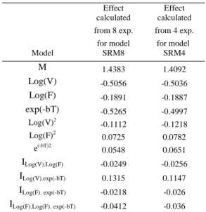
TABLEVIII
EFFECT VALUES FOR THE LIFESPAN MODEL, VECTOR Ê
Model Effect calculated from 8 exp. for model SRM8 Effect calculated from 4 exp. for model SRM4 M 1.4383 1.4092 Log(V) -0.5056 -0.5036 Log(F) -0.1891 -0.1887 exp(-bT) -0.5265 -0.4997 Log(V)2 -0.1112 -0.1218 Log(F)2 0.0725 0.0782 e(-bT)2 0.0548 0.0651 ILog(V).Log(F) -0.0249 -0.0256 ILog(V).exp(-bT) 0.1315 0.1147 ILog(F). exp(-bT) -0.0218 -0.026 ILog(F).Log(F). exp(-bT) -0.0412 -0.036
The vector effect Ê is then calculated with the mean square fit, as expressed in (10)
Ê = (XtX)-1. Xt.Y (10) Vector Y could be either the 13° column of Table VII
when taking into account the full experimental results or the 14° column of Table VII in case of a reduced set of experiments. Fig. 4 shows for example the non linearity of the response surface associated to model xx, limited to the most influent factors, i.e. V and T.
Fig. 4. Response surface diagram for 2 parameters, V and T, out of the 3 parameters involved in the model (V, F and T).
Other experiments inside the experimental domain are carried out such as the 11 points in Table IX, in order to check the models validity. It presents and compares the different results obtained with different models:
• DoE model has been built from 8 experiments focusing only on the main influential factors and interactions,
• SRM8 model relies on 8 experiments and includes only the most influent factors,
• SRM4 model is only based on 4 experiments randomly chosen out of the 8 experiments of SRM8 model and includes only the most influent factors. It turns out that the use of the SRM increases the model precision and that a limited number of experiments (4 instead of 8) do not dramatically affect the corresponding model precision.
TABLE IX
EXPERIMENTAL POINTS FOR MODEL VERIFICATION I.E. POINTS INSIDE THE EXPERIMENTAL DOMAIN BUT NOT INCLUDED IN TABLE II AND III
V level F level T level Weibull Exp. Result (8 exp.) DoE Model (8 exp.) % Diffe- rence SRM8 Model (8 exp.) % Diffe- rence SRM4 Model (4 exp.) % Diffe- rence 2kV; 10 kHz; 117.5 °C 0.262 0.262 0.694 1.017 0.920 -9.5% 0.937 -7.9% 0.928 -8.4% 1kV; 5kHz; 20°C -1 -1 -0.061 2.089 2.206 5.6% 2.137 2.3% 2.098 0.7% 2kV; 10kHz; 100°C 0.262 0.262 0.587 1.069 0.974 -8.9% 0.982 -8.1% 0.970 -9.4% 1.7 kV; 15 kHz; 26.7°C 0 1 0 1.314 1.266 -3.6% 1.321 0.5% 1.298 2.1% 1.7 kV; 8.6 kHz; 180°C 0 0 1 0.997 0.924 -7.4% 0.970 -2.7% 0.978 4.1% 3 kV; 8.7 kHz; 26.7°C 1 0 0 0.881 0.935 6.0% 0.822 -6.7% 0.785 -3.7% 2kV; 10kHz; 62.5°C 0.262 0.262 0.320 1.165 1.109 -4.9% 1.101 -5.5% 1.081 -7.4% 1.5 kV; 7.5 kHz; -17.5°C -0.262 -0.262 -0.481 1.771 1.915 8.1% 1.901 7.4% 1.858 5.3% 1kV; 8.6 kHz; 26.7°C -1 -0.013 0.004 1.769 1.976 11.7% 1.833 3.6% 1.791 2.3% 1.73 kV; 5 kHz; 26.7°C 0 -1.000 0 1.704 1.642 -3.7% 1.699 -0.3% 1.675 -1.2% 1.73kV; 8.6kHz; -55°C 0 0 -1 1.986 1.993 0.4% 2.023 1.9% 1.978 -1.1% 0,6 1,2 1,8 --1 0 1 8 2,4 -1 1 0 1 Weibull T V
VI. CONCLUSION
This paper has improved the previous work on lifespan modeling of the insulation of low voltage machines with the help of some statistical tools such as response surface and analysis of variance. It has been shown how the most influential factors can be identified, that the SRM increases modelling accuracy and that an experiment number reduction is possible with low risks.
The final objective of this work is to extend the validity domain of the model, primarily towards low constraint levels, for prognostic purposes. Other constraints such as pressure will be included in future work.
VII.REFERENCES
[1] P.J. Tavner, “Review of condition monitoring of rotating electrical machines”, IET Electr. Power Appl., vol. 2, no. 4, pp. 215–247, 2008.
[2] J. Yang, S.B. Lee, J. Yoo, S. Lee,Y. Oh, C. Choi, "A Stator Winding Insulation Condition Monitoring Technique for Inverter-Fed Machines", IEEE Trans. Power Elec., vol. 22, no. 5, pp 2026-2033, 2007.
[3] G. Mazzanti, “The combination of electro-thermal stress, load cycling and thermal transients and its effects on the life of high voltage ac cables”, IEEE Trans. Dielec. and Elec. Insul. vol. 16, no.4, pp. 1168–1179, 2009.
[4] J.P Crine, “On the interpretation of some electrical aging and relaxation phenomena in solid dielectrics”, IEEE Trans. Dielec. Elec. Insul., vol. 12, no. 6, pp. 1089-1107, 2005.
[5] R. Bartnikas, R. Morin, “Multi-stress aging of stator bars with electrical, thermal, and mechanical stresses as simultaneous acceleration factors, IEEE Trans. Ener. Conv., vol. 19, no. 4, pp. 702–714, 2004.
[6] Smet, F. Forest, J. Huselstein, and F. Richardeau, “Diagnosiss for Electric Machines, Power Electronics & Drives”, in Proc. IEEE SDEMPED, 2011, pp. 278–282.
[7] F. Guastavino, A. Ratto, E. Torello, G. Biondi, G. Loggi, and A. Ceci, “Electrical aging tests on different nanostructured enamels subjected to severe voltage waveforms”, Proc. IEEE SDEMPED, 2011, pp. 278–282.
[8] R.A. Fisher, The Design of Experiments, Edinburgh, Oliver and Boyd, 1935.
[9] I.P. Brown, and R.D. Lorenz, “Induction Machine Design Methodology for Self-Sensing: Balancing Saliencies and Power Conversion Properties”, IEEE Trans. Ind. Appl., vol. 47 , no. 1, pp. 79–87, 2011.
[10] M.S. Islam, R. Islam, T. Sebastian, A. Chandy, and S.A. Ozsoylu, “Cogging Torque Minimization in PM Motors Using Robust Design Approach”, IEEE Trans. Ind. App., vol. 47, no. 4, pp. 1661–1669, 2011.
[11] S. R. Cove, M. Ordonez, F. Luchino and John E. Quaicoe, “Applying Response Surface Methodology to Small Planar Transformer Winding Design", IEEE Trans. Ind. Electron., vol. 60, no.2, pp 483-493, 2013.
[12] H.M. Hasanien, and S.M Muyeen, “Design Optimization of Controller Parameters Used in Variable Speed Wind Energy Conversion System by Genetic Algorithms”, IEEE Trans. on Sust. Energy, vol. 3, no. 2, pp. 200 – 208, 2012.
[13] S. Rahmani, N. Mendalek, K. Al-Haddad; “Experimental Design of a Nonlinear Control Technique for Three-Phase Shunt Active Power Filter”, IEEE Trans. Ind. Elec., vol. 57, no. 10, pp 3364–3375, 2010. [14] Lahoud, N.; Faucher J.; Malec, D.; Maussion, P., « Electrical Aging
of the Insulation of Low Voltage Machines: Model definition and test with the Design of Experiments”, Industrial Electronics, IEEE Transactions on, vol. pp, no. 99, 2013, pp 1
[15] B. Bertsche, Reliability in Automotive and Mechanical Engineering Determination of Component and System Reliability, Springer, 2008. [16] N. Lahoud; J. Faucher; D. Malec, and P. Maussion, “Electrical ageing
modeling of the insulation of low voltage rotating machines fed by inverters with the design of experiments (DoE) method”, in Proc. IEEE SDEMPED, 2011, pp. 272–277.
[17] M. Pillet, Les plans d’expériences par la méthode Taguchi, Paris, Les Editions d’Organisation, 2001.
[18] Kim, S-I. I.; Kim, Y-K ; Lee, G-H ; Hong, J-P P, “A Novel Rotor Configuration and Experimental Verification of Interior PM Synchronous Motor for High-Speed Applications”, Magnetics, IEEE Transactions on vol. 48 , Issue: 2, 2012 , pp. 843 – 846
[19] Sahin, S.; Isler, Y., “Microcontroller-Based Robotics and SCADA Experiments”, IEEE Trans. on Education, vol. PP, no. 99, 2013, p 1 [20] Vergura, S.; Acciani, G.; Amoruso, V.; Patrono, G. E.; Vacca, F.,
“Descriptive and Inferential Statistics for Supervising and Monitoring the Operation of PV Plants”, Industrial Electronics, IEEE Trans. on, vol. 56, 2009 , pp. 4456 – 4464
[21] S. Shapiro and M. Wilk, “An analysis of variance test for normality”, Biometrika, vol. 52, no. 3, pp 591-611, 1965.
[22] Myers R.H and Montgomery D.C., Response Surface Methodology, J. Wiley and Sons, 2002
[23] Versèle, C.; Deblecker, O.; Lobry, J., “A Response Surface Methodology Approach to Study the Influence of Specifications or Model Parameters on the Multiobjective Optimal Design of Isolated DC–DC Converters”, Power Elec.s, IEEE Trans.s on, vol. 27, no. 7, 2012, pp. 3383 – 3395
[24] Hasanien, Hany M., “Particle Swarm Design Optimization of Transverse Flux Linear Motor for Weight Reduction and Improvement of Thrust Force”, Industrial Electronics, IEEE Transactions on, vol. 58 , no. 9, 2011 , pp. 4048 – 4056
VII. BIOGRAPHIES
Antoine Picot graduated from National Polytechnique Institut (INP) Grenoble, France in 2006. He received the M degree in signal, image, speech processing in 2006 and his PhD in control and signal processing in 2009 from the INP Grenoble. He is actually associate professor at the INP Toulouse. His research interests are in monitoring and diagnosis of complex systems with signal processing and AI techniques.
David Malec was born in France in 1964. He got the Eng. degree in 1992 from the Conservatoire National des Arts et Métiers and the Ph.D. degree in 1996 from Paul Sabatier University of Toulouse, where he is Professor in Electrical Engineering. His scientific activities deal with the study of solid insulating materials (polymers and ceramics) used in both low and high voltage electrical engineering domains.
Pascal Maussion (member IEEE) got his MSc and PhD in Electrical Engineering in 1985 and 1990 from Institut National Polytechnique (Toulouse, France). He is currently Professor with the University of Toulouse and LAPLACE, Lab. for PLAsma and Conversion of Energy. His research activities deal with control and diagnosis of electrical systems and with the design of experiments for optimisation. He is currently head of Control and Diagnosis group and teaches control and diagnosis.