HAL Id: hal-01201226
https://hal.archives-ouvertes.fr/hal-01201226
Submitted on 15 Apr 2020
HAL is a multi-disciplinary open access
archive for the deposit and dissemination of
sci-entific research documents, whether they are
pub-lished or not. The documents may come from
teaching and research institutions in France or
abroad, or from public or private research centers.
L’archive ouverte pluridisciplinaire HAL, est
destinée au dépôt et à la diffusion de documents
scientifiques de niveau recherche, publiés ou non,
émanant des établissements d’enseignement et de
recherche français ou étrangers, des laboratoires
publics ou privés.
Integrating spatial information into probabilistic
relational model
Rajani Chulyadyo, Philippe Leray
To cite this version:
Rajani Chulyadyo, Philippe Leray. Integrating spatial information into probabilistic relational model.
2015 IEEE International Conference on Data Science and Advanced Analytics (IEEE DSAA’2015),
2015, Paris, France. �10.1109/DSAA.2015.7344800�. �hal-01201226�
Integrating Spatial Information into
Probabilistic Relational Models
Rajani Chulyadyo
LINA UMR 6241, DUKe Research Group DataForPeople
Nantes, France
Email: [email protected]
Philippe Leray
LINA UMR 6241, DUKe Research Group Nantes, France
Email: [email protected]
Abstract—Growing trend of using spatial information in vari-ous domains has increased the need for spatial data analysis. As spatial data analysis involves the study of interaction between spatial objects, Probabilistic Relational Models (PRMs) can be a good choice for modeling probabilistic dependencies between such objects. However, standard PRMs do not support spatial objects. Here, we present a general solution for incorporating spatial information into PRMs. We also explain how our model can be learned from data and discuss on the possibility of its extension to support spatial autocorrelation.
I. INTRODUCTION
Availability of GPS to civilian users, advances in mobile communication and wireless technology have opened the door to many spatial technologies. The development of consumer GPS tools, Volunteered Graphical Information (VGI) tools and location-aware mobile devices have revolutionized the way of collecting and using location information. The growing trend of using spatial information/databases in a wide range of application domain has increased the need for analysis of spatial data.
Spatial data analysis is certainly not a new field [1]. Several methods have been devised to extract patterns from spatial data and understand underlying phenomena [2], [3]. A Bayesian network is one of such methods that have been used with spatial information in various domains [4], [5], [6], [7], [8], [9], [10] for dependency analysis. Recently, object-oriented Bayesian networks have also been used for modeling spatial interactions [5]. However, these approaches are mostly dedicated for specific problems, and many of them do not capture spatial dependencies well. [4]’s approach to modeling spatial dependencies sounds appealing as they present some promising results with their intuitive approach. They auto-matically learn Bayesian networks from data, limiting spatial dependencies within the vicinity of nodes.
Most of the techniques of spatial data analysis work with flat representation of data. However, real-world applications are generally conceptualized in terms of objects and relations between them, and, hence, data need to be transformed into the required flat format before applying those methods. Besides, analysis of spatial information usually involves the study of interaction between spatial objects. In such relational domains, Probabilistic Relational Models (PRMs) [11] can be employed
to learn probabilistic models. A PRM is a relational extension of Bayesian Networks and models the uncertainty over the attributes of objects in the domain and the uncertainty over the relations between the objects. However, standard PRMs do not support spatial objects. Therefore, we aim at integrating spatial information into PRMs to enable them to handle spatial objects too. Our motivation is also driven by [12]’s perspective on spatial data mining in relational domain. In their paper [12], the authors argue that multi-relational setting is the most suitable for spatial data mining problems and also mention the possibility of using PRMs with spatial relational databases. This view has also been supported by several works [13], [14] not related to PRMs.
We propose to extend standard PRMs to support spatial objects. Our model provides a general way to incorporate spa-tial information into a PRM and model spaspa-tial dependencies. In this paper, we are mainly concerned with geographically referenced objects and deal with vector representation of spatial data, where a spatial object is described by its attributes and its geometry. Though the attributes of spatial objects can be modeled by descriptive attributes in standard PRMs, their geometry cannot be modeled in PRMs in a straightforward manner because the geometry can be as simple as points, which can be described by a pair of coordinates, and also as complex as lines and polygons, which are represented by a sequence of pairs of coordinates. Thus, spatial geometry attributes cannot be treated as simple continuous variables.
One approach to support spatial objects in PRMs is to parti-tion spatial geometry attributes and learn a regular PRM from data using the partitions. However, with this approach, we may miss some useful probabilistic dependencies because the same partitioning level may not be appropriate to detect dependen-cies of the partitioned attribute with any attributes. Thus, we propose a different approach where the partitioning of spatial geometry attributes is interleaved with the learning process. We first adapt the relational schema for spatial attributes and then define a model over the adapted relational schema. While learning the model from data, adaptative partitioning is performed on spatial geometry attributes to find the partitions that best describe dependencies. We present two different approaches to adapt the partitioning process. We should note here that the partitioning of spatial geometry attributes is
different from discretization of continuous variables in that the former results into spatial objects again. For instance, the partitioning of a set of spatial point objects might result into a set of spatial polygon objects. Because the spatial attributes are not disregarded after partitioning, the model can be further enhanced by adding a support for spatial functions to explore more useful attributes from spatial attributes. We also point to the possibility of modeling spatial autocorrelation [15] with our model. Though spatial autocorrelation cannot be modeled directly in PRMs because of acyclicity constraint [16], we present our idea of modeling spatial autocorrelation by introducing (or deriving) aggregated attributes and adding a special constraint on the orientation of edges between the aggregated attribute and the original attribute to avoid cycles. This paper is organized as follows. In section 2, we present a brief overview of spatial data and PRMs. In section 3, we present our model in detail and illustrate the model with an example. We discuss about the model in section 4 and finally conclude the paper with our future perspective on the model.
II. BACKGROUND
A. Spatial data
Tessellations and vectors are two basic data types used to represent spatial information though network data type has also been reported in some literature [3]. In the tessellation representation of spatial data, the space is partitioned into mutually exclusive cells that together make up the complete coverage. Each cell is associated with thematic/attribute values that represent the conditions for the area covered by that cell. In the vector data representation, spatial objects are modeled using geometry and their attributes. The geometry is made up of one or more interconnected vertices. A vertex describes a position in space using an x, y and optionally z axis. Spatial objects can be zero-dimensional (point), 1-dimensional (line) or 2-dimensional (surface).
B. Probabilistic Relational Model (PRM)
A probabilistic relational model (PRM) [17], [11] is a formal approach to relational learning. It defines a template for probability distributions over relational domains. PRMs can be later instantiated with a particular set of objects and relations between them to obtain a Bayesian Network which defines probability distributions over the attributes of the objects. A PRM is comprised of two components: a relational schema of the domain and a probabilistic model.
a) Relational schema: A relational schema describes a set of classes and the relationships between them. Each class X ∈ X is described by a set of descriptive attributes A(X) and a set of reference slots R(X). The attributes X.Ai are
random variables with states from a discrete domain V(X.Ai).
A reference slot X.ρ that relates an object of class X to an object of class Y has Domain[ρ] = X and Range[ρ] = Y . The inverse of a reference slot ρ is called inverse slot and is denoted by ρ−1. In the context of relational databases, a class refers to a single database table, descriptive attributes refer to the standard attributes of tables, and reference slots
are equivalent to foreign keys. While a reference slot gives a direct reference of an object with another, objects of one class can be related to objects of another class indirectly through other objects. Such relations are represented with the help of a slot chain – a sequence of slots (reference slots and inverse slots) ρ1, ρ2, . . . ρn such that for all i, Range[ρi] =
Domain[ρi+1]. Slot chains may lead to one-to-many or
many-to-many relations, in which case we need an aggregator, i.e. a function, denoted γ, which takes a multi-set of values and produces a single value (e.g., average, mode, cardinality etc.) as a summary of the set of related objects.
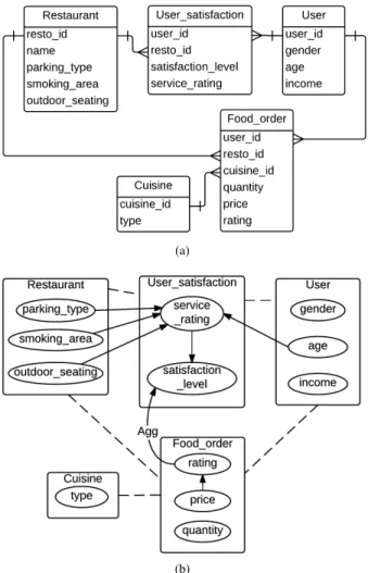
To illustrate these concepts, we use a relational schema of a system where users order foods in restaurants and rate the service of the restaurants. The schema is shown in figure 1a. We will refer to the same sys-tem throughout the paper to give examples. Here, Restau-rant, User and Cuisine are also called entity classes.
User satisfaction and Food order are called relationship classes because they represent the relationships Restaurant–
User and User–Cuisine respectively. The attributes User.age,
User.gender, User satisfaction.service rating etc. are descrip-tive attributes whereas User satisfaction.user id, which refers to User.user id, is a reference slot whose domain and range are User satisfaction and User respectively. Here, Restaurant
and User satisfaction objects are directly linked through the reference slot User satisfaction.resto id. Note that Restau-rant.resto id−1 is the inverse of User satisfaction.resto id
and gives all User satisfaction objects corresponding to
Restaurant objects. Restaurant objects can also be in-directly related to User objects through the slot chain
User satisfaction.resto id−1.user id, which gives all the users whose satisfaction level and/or service rating about the restau-rants are available. As there is a many-to-many relationship between the classes RestaurantandUser, this slot chain may result into more than one user for a single restaurant. In such case, we need an aggregator (such as average) to sum-marize (or aggregate) the resulting set. For instance, AVER-AGE(User satisfaction.resto id−1.user id.age) gives the aver-age aver-age of the users who have rated the restaurants.
b) Probabilistic model: A PRM specifies a probabilistic modelfor classes of objects. It represents generic probabilistic dependencies between the attributes of classes in the relational schema. The dependencies can be between the attributes of the same class or between the attributes of different classes. Like in Bayesian networks, the dependency structure is associated with the conditional probability distribution of each node (attribute) given its parents.
Figure 1b depicts a PRM that corresponds to the relational schema in 1a. Here, the dashed lines indicate that the classes are linked through reference slots in the relational schema, and the edge with ’Agg’ denotes that the child node depends on the aggregated value of the parent node.
Formally, a regular PRM Π for a relational schema R is defined as follows [11]. For each class X ∈ X and each descriptive attribute A ∈ A(X), we have:
(a)
(b)
Fig. 1. (a) An example of a relational schema of a system where users orders foods in restaurants and rate the services of the restaurants. The relationships between classes are denoted by the lines connecting them, and the type of their relationships is given by the line ends, e.g. the class
Restaurant has a one-to-many relationship with the class User satisfaction. (b) A PRM that corresponds to the relational schema in 1a. Each descriptive attribute is denoted by a node. The directed edges between the nodes represent probabilistic dependencies between the nodes. The dashed lines between the classes indicate that the classes are related to each other through reference slots in the relational schema. An aggregator is indicated by ‘Agg’ in an edge. An aggregated dependency is present in the edge fromFood order.rating to
User satisfaction.satisfaction level, which means that the users’ satisfaction level depends probabilistically on the aggregated value of their rating on foods ordered by them.
has the form X.B or γ(X.τ.B), where B is an attribute of any class, τ is a slot chain and γ is an aggregator of X.τ.B.
• a conditional probability distribution (CPD),
P (X.A|P a(X.A)).
Probabilistic inference is performed on a Ground Bayesian Network (GBN) obtained by instantiating a PRM for a partic-ular instance I of the associated relational schema (i.e. a set of objects and relations between them). It specifies probability distributions over the attributes of the objects. A GBN has a node for every attribute of every object in I, and probabilistic dependencies and CPDs as in the PRM. As GBNs tend to be very big, standard inference algorithms for Bayesian networks
need to be adapted to infer the value of unobserved attributes [11].
Learning a PRMinvolves two tasks – parameter estimation and structure learning. The aim of parameter estimation is to find parameters θs that define CPDs for a dependency
structure S given a complete instantiation I. While learning the structure of a PRM, we need to make sure that the structure is not only legal (i.e. acyclic) but also the best one among the candidate structures. [11] propose to apply greedy hill-climbing algorithm over relational attributes (limiting the max-imum length of slot chain) to explore structure search space and use a Bayesian scoring function to evaluate legal candidate structures. While exploring and evaluating structures, one needs to compare score of structures with only small local differences (e.g., comparing a structure with another structure obtained from it by adding only one edge between two nodes). In such case, a decomposable Bayesian scoring function can simplify the computation because it allows computing the separate contribution of each variable to the quality of the network so that it will be sufficient to compute the score of only those terms that involve the variables being modified instead of computing score of the complete structure again. A scoring function is decomposable if the global score assigned to a Bayesian network B with N nodes for the given data D can be represented as a sum of local score that depends only on each node Xi and its parents P a(Xi), i.e.,
(Global)Score(B, D) =
N
X
i=1
(local)Score(Xi|P a(Xi)) (1)
III. PRMWITH SPATIAL ATTRIBUTES(PRM-SA) We begin by defining some basic concepts related to our model. We, then, define our model and illustrate the model with examples. Then we explain how to learn our model. A. Definitions
We propose to incorporate the vector representation of spatial objects, where a spatial object is described by its location in space in terms of geometry and its attributes, in PRMs. The attributes of a spatial object can form descriptive attributes in the relational schema whereas its geometry cannot be incorporated as descriptive attributes because the geometry of spatial objects is represented by a set of points (vertices or coordinates). Thus, we coin a term spatial geometry attribute or simply spatial attribute to describe such attributes to use them in a PRM.
Definition 1: Spatial geometry attribute
An attribute is a spatial geometry attribute if its value s is a sequence of pairs of coordinates in geographic coordinate reference systems and defines the geometry of its class. i.e. s = ((x, y)n : n ∈ N) where x is called longitude, y is called
latitudeand n is the cardinality of s. Here, s represents
• a point geometry if n = 1,
• a line geometry if n ≥ 2 and s16= sn , • a polygon geometry if n ≥ 2 and s1= sn.z
Definition 2: Spatial class
Let SA(X) be the set of spatial geometry attributes in a class X. A class X is a spatial class if SA(X) is not empty. z
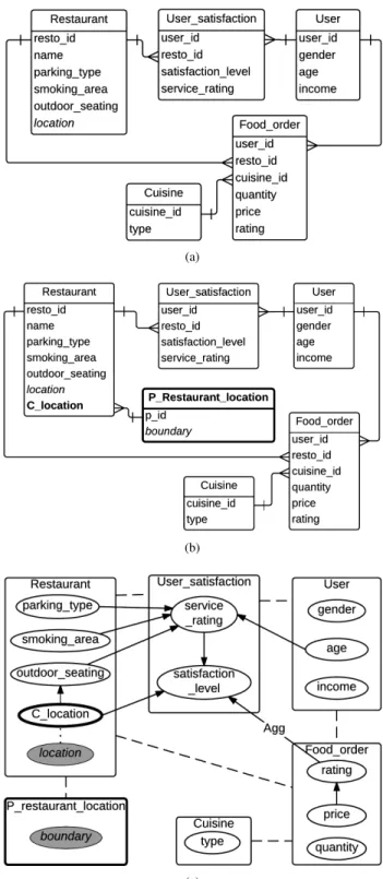
To illustrate these concepts, we refer to the system in figure 1 and extend the relational schema in figure 1a with a spatial geometry attribute in the class Restaurant as shown in figure 2a. Here, the spatial attributeRestaurant.locationrepresents the location of the objects of the spatial classRestaurant.
As the set of possible values of a spatial attribute is infinite, conditional probability distributions associated with spatial attributes would be very big. It demands an extensive computation for learning as well as inference and this is practically too difficult to achieve. Therefore, we propose to partition this set into a finite number of disjoint subsets with the help of a spatial partition function. Each partition is then represented by a class, which we call a spatial partition class, and a reference slot (we call it a spatial reference slot or spatial ref. slot) that refers to the objects of the partition class is added in the corresponding spatial class. Partition functions are responsible for creating the objects of partition classes and mapping the values of a spatial attribute to their corresponding partitions.
Definition 3: Spatial partition function, Spatial partition class
Let X.SA be a spatial geometry attribute of a spatial class X. We define a spatial partition function fsa : X.SA →
Range[fsa] where Range[fsa] is a finite set of spatial
parti-tions represented by a spatial partition class PXSA. Thus, fsa
associates each sa ∈ Domain[X.SA] to an object of PXSA
determined by the function itself.z
Partition functions essentially map a spatial object to a region such that spatial objects meeting some partitioning criteria are grouped together. Such mapping can be achieved in many ways. One way is to use regular square or hexagonal (honeycomb) grids to partition the spatial region. Partitions can also be created by using standard, publicly available knowledge such as administrative boundaries. In the absence of such knowledge, spatial clustering algorithms can be used. [18] have presented a survey on several spatial clustering methods. Some clustering algorithms, such as K-means, re-quire users to provide the number of clusters/regions and some others, such as DBSCAN, can determine the number of clusters themselves. It should be noted that granularity of partitioning methods depends on the context of the problem. Also note that when using knowledge to create partitions, we may have access to some extra information. Such information can be considered as descriptive attributes of partition classes. The introduction of partition classes enables us to implement hierarchical clustering as well because partition classes can contain spatial attributes, which can be further partitioned thereby creating a hierarchy of spatial partition classes.
We refer to figure 2a for examples. As the spatial attribute
Restaurant.location can take infinitely many values, we define a partition function to partition its possible values into a finite set of spatial partitions. Thus, we add a spatial
par-(a)
(b)
(c)
Fig. 2. (a) An example of a relational schema with a spatial attribute
Restaurant.location, which cannot be handled by standard PRMs. (b) The relational schema adapted for the spatial attribute Restaurant.location as proposed in definition 4.1. Here, spatial attributes are shown in italicized font and the added spatial reference slot and the spatial partition class are shown in boldface. (c) A PRM-SA as proposed in definition 4. The gray nodes are spatial attributes and the one with thick border is the spatial reference slot associated with the spatial attributeRestaurant.location. The dotted line between Restaurant.location and Restaurant.C location indicates that the spatial attribute and the spatial ref. slot are associated through a spatial partition function.
tition class P Restaurant location that represents the spatial partitions of Restaurant.location. The objects of this spatial partition class will then be referenced in the spatial class
Restaurantby the spatial reference slotRestaurant.C location. Figure 2b shows the relational schema adapted for the spatial attribute. Here, we have assumed that the spatial partition class will have an additional attribute calledboundary, which is again a spatial attribute. In this example, we can assume that this attribute represents the convex hull formed by all the locations mapped to the particular partition object. How-ever, the attributes present in the partition classes depend on the context. If we use the information about administrative boundaries of cities or regions,P restaurant location.boundary
might represent the boundary of the specified location, and we might even have extra information about the partitions such as population, average income, demographic structure etc. of the location. If hierarchical administrative division is available, we can incorporate hierarchical partitions by further partitioning
P restaurant location.boundary and adding another partition class, say P restaurant location boundary (not shown in the figure).
We now define our model, which is based on standard PRMs and supports spatial data.
Definition 4: PRM with spatial attributes (PRM-SA) Let A(X) and SA(X) denote the set of descriptive at-tributes and geometry atat-tributes respectively in class X.
For each spatial class X ∈ X such that SA(X) 6= ∅ and for each geometry attribute SA ∈ SA(X), we define the following:
• a new partition class PXSA,
• a partition function fsa : SA → PXSA that creates
instances of PXSA associating each sa ∈ Domain[SA]
to one of the instances of PXSA, and
• a new spatial reference slot X.CSAassociated with fsa.
Then, we adapt the relational schema for spatial attributes and define the probabilistic model in the following way.
Definition 4.1: Adapted relational schema
The relational schema is adapted for spatial attributes by adding PXSAand X.CSAassociated with fsafor each spatial
class X ∈ X and for each geometry attribute SA ∈ SA(X). Definition 4.2: Probabilistic model of a PRM-SA
Let PSAand CSAbe the set of partition classes and the set
of added spatial reference slots respectively. Then, for each class X ∈ {X ∪ PSA} and each attribute A ∈ {A(X) ∪
CSA(X)}, we have
• a set of parents P a(X.A) = {U1, ..., Ul}, where each Ui
has the form X.B or γ(X.K.B), where B is an attribute of any class, K is a slot chain and γ is an aggregate of X.K.B,
• a legal conditional probability distribution CPD, P (X.A|P a(X.A)).z
A PRM-SA that corresponds to the schema in figure 2a is shown in figure 2c. Here, the gray nodes are spatial attributes and the nodes/classes with thick border are the ones that are not present in the original relational schema. The probabilistic dependencies shown in the examples are hypothetical.
Probabilistic inference is performed on a ground Bayesian network (GBN) obtained by instantiating a PRM-SA for a given relational skeleton. Here, the skeleton must also include the objects of spatial classes. Given such a relational skeleton, a PRM-SA induces a GBN that specifies probability distribu-tions over the attributes of the objects. Here, we need to ensure that the probability distributions are coherent, i.e. the sum of probability of all instances is 1. In Bayesian networks, this requirement is satisfied if the dependency graph is acyclic [19]. Following [11]’s approach, we consider instance dependency graphto check whether the dependency structure S of a PRM-SA is acyclic relative to a given relational skeleton. Due to the presence of spatial attributes, standard instance dependency graphs need to be redefined with some adaptations for PRM-SA but we can still follow [11]’s proof to show that the dependency structure S for a PRM-SA is guaranteed to be acyclic for the given relational skeleton if the corresponding instance dependency graph is acyclic.
Definition 5: Instance dependency graph (IDG)
The instance dependency graph Gσr for a PRM-SA Π with
partition classes PSA and a relational skeleton σr is defined
as follows. For each object x ∈ σr(X) in each class X ∈
{X ∪ PSA}, we have the following nodes: a node x.A for
each descriptive attribute X.A, and a node x.CSA for each
spatial reference slot X.CSA. The graph has the following
edges:
1) Type I edges: For each formal parent of x.A, X.B, we introduce an edge from x.B to x.A.
2) Type II edges: For each formal parent X.K.B, and for each y ∈ x.K, we define an edge from y.B to x.A. 3) Type III edges: For any spatial attribute x.SA in each
spatial class X ∈ X , we define an edge x.SA → x.CSA.
4) Type IV edges: For any attribute p.A in each spatial partition class P ∈ PSA and p ∈ σr(P ), we add an
edge p.A ← x.A if P.A is derived from X.A. z Following [11] again, we can demonstrate that the prob-abilistic model of a PRM-SA is coherent for any relational skeleton if the corresponding class dependency graph is acyclic. Here again, because of the presence of spatial at-tributes, we redefine class dependency graph for PRM-SA.
Definition 6: Class dependency graph (CDG)
The class dependency graph GΠfor a PRM-SA Π is defined
as follows. The dependency graph has the following nodes: a node for each descriptive attribute X.A, and a node for each spatial reference slot X.CSA. The graph has the following
edges:
1) Type I edges: For any attribute X.A and its parent X.B, we introduce an edge from X.B to X.A.
2) Type II edges: For any attribute X.A and its parent X.K.B, we introduce an edge from Y.B to X.A, where Y = Range[X.K].
3) Type III edges: For any spatial attribute X.SA in each spatial class X ∈ X , we define an edge X.SA → X.CSA.
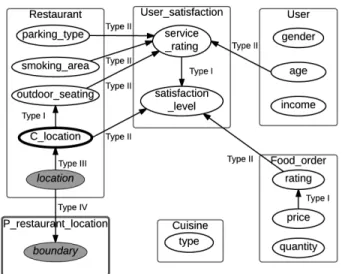
Fig. 3. The class dependency graph for the PRM-SA in figure 2c. Because there is no cycle in this graph, we can conclude that the dependency structure in figure 2c is acyclic for any relational skeleton.
Fig. 4. An example of a class dependency graph with a cycle. Because of the presence of a cycle, we can conclude that the dependency structure cannot be guaranteed to be acyclic for any relational skeleton.
4) Type IV edges: For any attribute P.A in each spatial partition class P ∈ PSA, we add an edge P.A ← X.A
if P.A is derived from X.A.z
Figure 3 shows the class dependency graph for the PRM-SA in figure 2c. Because this graph is acyclic, the dependency structure in figure 2c is guaranteed to be acyclic regardless of relational skeleton.
Let us consider another hypothetical example where there is an attributeUser.locationand a partition classP User location
that represents the partitions of users’ location. Suppose there exists a dependency that says the income of a user depends on the average income of the users in his community, i.e. users with similar income tend to live in the same community. In this case, the dependency structure of a PRM-SA will have an edge from P User location.avg income to User.income. Although there is no cycle in the structure, it is incoherent because the class dependency graph of this structure contains a cycle as shown in figure 4. This is due to the type IV edge that is added becauseP User location.avg incomeis derived from
User.income.
B. Learning PRM-SA
As with standard PRMs, learning a PRM-SA involves the tasks of parameter estimation and structure learning. Parame-ters of a PRM-SA can be learned in the same way as for a regular PRM. However, the instances of all partition classes must be included in the instantiation of the relational schema. As for structure learning, following [17]’s approach, we apply relational greedy search algorithm to explore the search space of candidate structures and evaluate legal can-didate structures using score-based methods. However, due to the introduction of partition classes along with partition functions, we need to adapt the search algorithm to deal with partitions. Here, we come across two situations – 1) when the number of partitions of the spatial attribute (i.e. Cardinality(Range[fsa]), let’s denote it by ksa) is known,
and 2) when it is unknown. In the former case, standard relational greedy search algorithm can be applied to explore the search space. However, the situation is complicated in the latter case where the number of partitions needs to be determined by the algorithm.
We present two approaches to learn a PRM-SA when ksa
is unknown. A naive way is to add new operators increase k and decrease k, which increases or decreases the number of partitions respectively, and use these operators along with add, delete and revert edge operators of standard greedy search algorithm to find neighborhood of a structure. In our second approach, we separate the tasks of greedy search over candidate structures and finding the optimal number of partitions of spatial attributes. The basic idea is to pick the best scoring structure among candidate structures, and then find the optimal number of partitions of the spatial attributes in this structure if this structure is obtained by changing (i.e. adding, deleting or reverting) an edge that involves a spatial reference slot. To simplify the computation, we use a decomposable Bayesian scoring function. So, it is sufficient to compute the score of only those terms that involve the variables being modified.
An important point to note here is that if a spatial reference slot appears with other spatial reference slots in the local score terms of the scoring function (while finding the optimal number of partitions), we need to vary the cardinality of the set of all spatial reference slots that appear together with the target spatial reference slot. To visualize this concept, we propose to moralize1the structure and find 2-vertex cliques of spatial
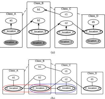
ref-erence slots. Those connected through the cliques form a set of variables whose cardinality should be varied altogether when optimizing the number of partitions. This concept is illustrated in figure 5. Note that spatial partition classes associated with each spatial attributes exist here but they are not shown in the diagram to save some space. Suppose the PRM-SA in figure 5a is obtained at some point during structure learning by adding
1A moral graph is the equivalent undirected graph of a directed acyclic
graph and is obtained by adding an edge between the nodes that have a common child and changing directed edges to undirected ones.
(a)
(b)
Fig. 5. (a) A PRM-SA with multiple spatial attributes. (b) The correspond-ing moralized graph used to identify the set of partition functions to be optimized. Here, the pairs of spatial reference slots {Class A.C location a,
Class B.C location b} and {Class B.C location b, Class C.C location c} form 2-vertex cliques. Because these two cliques are connected, we need to find the optimal number of partitions for these three spatial ref. slots together.
an edge from Class A.C location a to Class A.a1. Because the added edge contains a spatial reference slot, we need to find the best number of partitions for this node. The score S of this structure is
S = S(Class A.a1|Class A.C location a)
+ S(Class A.C location a) + S(Class B.b1|Class C.c1) + S(Class B.b2|Class A.C location a,Class B.C location b) + S(Class C.c2|Class B.C location b,Class C.C location c) + S(Class C.c1) + S(Class D.d1|Class D.C location d) + S(Class D.C location d|Class C.c2) (2)
From equation 2, it is clear that changing the number of par-titions of Class A.C location aaffects the score of the nodes
Class A.a1 and Class B.b2. However, to find the best score for the nodeClass B.b2, we need to find the optimal number of partitions for Class B.C location b too because it appears with the spatial reference slot Class A.C location a in local score terms of the scoring function.Class B.C location balso appears withClass C.C location cin the scoring function. As a result, partition functions of all of the three spatial ref. slots need to be optimized together. To identify this set, we can moralize the dependency structure of the PRM-SA as shown in figure 5b and find out all 2-vertex cliques of spatial reference slots. The three spatial reference slots Class A.C location a,
Class B.C location b and Class C.C location c in figure 5b are connected through cliques. Therefore, we find the best
Fig. 6. An example of a dependency structure that models the dependency of an attribute with the aggregated value of the same attribute of spatial objects in the same cluster. This concept can be used to model spatial autocorrelation.
number of partitions for these three spatial reference slots altogether.
An interesting property of this approach of learning PRM-SA is that because of the separation of greedy search and partition size optimization, we can come up with different heuristics that involve different combinations of these two tasks. For example, we can perform one operation (add, delete or revert) of greedy search and then find the cardinality of spatial reference slots, or we can find the optimal cardinality of all spatial reference slots after a complete greedy search and so on. However, the best approach among these is yet to be discovered.
IV. DISCUSSION
Our model sounds somewhat similar to PRM with reference uncertainty (PRM-RU) [11] because the notion of partition and partition function has already been coined there. However, there is no reference uncertainty in our model. We partition spatial objects because the set of possible values of a geometry attribute is so big (or infinite) that specifying a probability distribution over the set of all values of a geometry attribute is too much of work. Unlike in PRM-RU, where more than one attribute (called partition attributes) can define a partition, there is only one partition attribute, i.e. the corresponding spatial attribute, for each partition class in our model. On the other hand, type III edges in IDG and CDG of our model correspond to type IV edges in those of PRM-RU.
Learning structure of our model when the number of partitions of spatial reference slots is unknown is inspired by standard methods of latent variable discovery in Bayesian networks [20]. We deal with the problem of finding the right dimensionality of special variables but these variables, in fact, are not latent. Thus, unlike in latent variable discovery techniques, we do not need to apply Expectation Maximization (EM) algorithm to score those special variables because our partition functions take care of providing complete data for those variables.
Researchers advocate the consideration of autocorrelation in spatial data analysis. However, autocorrelation cannot be mod-eled directly in PRMs because of acyclicity constraint [16]. An attribute of an instance depending on the same attribute of neighboring instances would create a cycle because of the fact that neighborhood is a mutual concept. Due to this reason, we do not model spatial autocorrelation directly. Nevertheless, it is still possible to extend our model to enforce the modeling of spatial autocorrelation by adding aggregated descriptive attributes in partition classes with a special constraint that the aggregated attribute must always be a child to ensure acyclicity. For example, let us consider the relational schema in figure 2a. Suppose there is an attribute User.location and a partition classP User locationthat represents the partitions of users’ location. Modeling spatial autocorrelation of users’ income (i.e. users’ income depending on the income of neigh-boring users) would create a cycle in the dependency structure. To avoid this, we could add an attribute avg income in the
P User location, which is, in fact, the average (aggregation) of User.income. P User location.avg income would, then, be enforced to be a child of User.income as shown in figure 6, otherwise we may come across the situation as in figure 4. This models the dependency of an attribute with the aggregated value of the same attribute of spatial objects in the same cluster. Relational Markov Networks (RMNs) could be another solution to model this spatial autocorrelation because depen-dencies are represented by an undirected graph in this type of probabilistic graphical models. However, learning RMNs is much more complex than learning PRMs.
V. CONCLUSION AND FUTURE WORK
In this paper, we have proposed a generic framework to incorporate spatial information into PRMs. Our model extends standard PRMs and provides a general solution to model spatial dependencies in PRMs. We have also presented our approaches to learning the model. Our model opens a possi-bility to model spatial autocorrelation with the introduction of aggregated attributes on partition classes and a special constraint on the orientation of edges to avoid cycles. Be-cause the spatial attributes are preserved in a PRM-SA, our model can be extended to support spatial functions that work directly with the spatial attributes. We are currently working to implement this model in PILGRIM, a software platform to work with probabilistic graphical models, being developed at our research lab, and to perform experiments to prove our concept. In future, we are planning to enhance this model with
[2] H. J. Miller and J. Han, Geographic data mining and knowledge discovery. CRC Press, 2009.
spatial functions to explore more meaningful attributes in the domain. We aim at applying this model in a recommender system for a real-world application.
REFERENCES
[1] M. F. Goodchild, “Twenty years of progress: GIScience in 2010,” Journal of Spatial Information Science, vol. 1, no. 1, pp. 3–20, 2010. [3] S. Shekhar, M. R. Evans, J. M. Kang, and P. Mohan, “Identifying
patterns in spatial information: A survey of methods,” Wiley Interdisci-plinary Reviews: Data Mining and Knowledge Discovery, vol. 1, no. 3, pp. 193–214, May 2011.
[4] R. Cano, C. Sordo, and J. Gutierrez, “Applications of Bayesian networks in meteorology,” Advances in Bayesian networks, pp. 309–327, 2004. [5] L. Wilkinson, Y. E. Chee, A. E. Nicholson, and P. F.
Quintana-Ascencio, “An Object-oriented Spatial and Temporal Bayesian Network for Managing Willows in an American Heritage River Catchment,” in UAI Application Workshops, 2013, pp. 77–86.
[6] L. Li, J. Wang, H. Leung, and C. Jiang, “Assessment of catastrophic risk using bayesian network constructed from domain knowledge and spatial data,” Risk Analysis, vol. 30, no. 7, pp. 1157–1175, 2010. [7] S. Sarkar and K. Boyer, “Integration, inference, and management of
spa-tial information using bayesian networks: perceptual organization,” IEEE Transactions on Pattern Analysis and Machine Intelligence, vol. 15, no. 3, pp. 256–274, Mar 1993.
[8] M.-h. Park, J.-h. Hong, and S.-b. Cho, “Location-Based Recommen-dation System Using Bayesian User’s Preference Model in Mobile Devices,” Ubiquitous Intelligence and Computing, pp. 1130–1139, 2007. [9] J. Huang and Y. Yuan, “Construction and Application of Bayesian Net-work Model for Spatial Data Mining,” in IEEE International Conference on Control and Automation. ICCA 2007, 2007, pp. 2802–2805. [10] A. R. Walker, B. Pham, and M. Moody, “Spatial Bayesian Learning
Algorithms for Geographic Information Retrieval,” pp. 105–114, 2005. [11] L. Getoor, “Learning Statistical Models from Relational Data,” PhD
Thesis, Stanford University, 2001.
[12] D. Malerba, “A relational perspective on spatial data mining,” Inter-national Journal of Data Mining, Modelling and Management, vol. 1, no. 1, pp. 103–118, 2008.
[13] M. Ceci and A. Appice, “Spatial associative classification: propositional vs structural approach,” Journal of Intelligent Information Systems, vol. 27, no. 3, pp. 191–213, 2006.
[14] D. Malerba, A. Appice, A. Varlaro, and A. Lanza, “Spatial clustering of structured objects,” in Inductive Logic Programming. Springer, 2005, pp. 227–245.
[15] D. A. Griffith, “What is spatial autocorrelation? Reflections on the past 25 years of spatial statistics,” Espace g´eographique, vol. 21, no. 3, pp. 265–280, 1992.
[16] J. Neville and D. Jensen, “Collective Classification with Relational Dependency Networks,” in Workshop on Multi-Relational Data Mining. KDD-2003, 2003, pp. 77–91.
[17] N. Friedman, L. Getoor, D. Koller, and A. Pfeffer, “Learning probabilis-tic relational models,” in IJCAI, vol. 16, 1999, pp. 1300–1309. [18] J. Han, M. Kamber, and A. K. H. Tung, “Spatial Clustering Methods in
Data Mining: A Survey,” in Geographic Data Mining and Knowledge Discovery, Research Monographs in GIS, H. J. Miller and J. Han, Eds. Taylor and Francis, 2001, pp. 1–29.
[19] L. Getoor, N. Friedman, D. Koller, and A. Pfeffer, “Learning Proba-bilistic Relational Models,” in Relational Data Mining, S. Dˇzeroski and N. Lavraˇc, Eds. Springer Berlin Heidelberg, 2001, pp. 307–335. [20] G. Elidan and N. Friedman, “Learning the Dimensionality of Hidden
Variables,” in UAI-2001. San Francisco, CA: Morgan Kaufmann Publishers, 2001, pp. 144–151.